Attributes and machine learning for fragment identification and malware analysis

Calhoun: The NPS Institutional Archive

Theses and Dissertations Thesis Collection

2014-09

Attributes and machine learning for fragment

identification and malware analysis

Beneduce, Kristen

Monterey, California: Naval Postgraduate School

NAVAL

POSTGRADUATE

SCHOOL

MONTEREY, CALIFORNIA

THESIS

ATTRIBUTES AND MACHINE LEARNING FOR FRAGMENT IDENTIFICATION AND MALWARE

ANALYSIS by

Kristen Beneduce September 2014

Thesis Advisor: Joel Young

Second Reader: Chris Eagle

REPORT DOCUMENTATION PAGE Form Approved OMB No. 0704–0188

Public reporting burden for this collection of information is estimated to average 1 hour per response, including the time for reviewing instruction, searching existing data sources, gathering and maintaining the data needed, and completing and reviewing the collection of information. Send comments regarding this burden estimate or any other aspect of this collection of information, including suggestions for reducing this burden to Washington headquarters Services, Directorate for Information Operations and Reports, 1215 Jefferson Davis Highway, Suite 1204, Arlington, VA 22202–4302, and to the Office of Management and Budget, Paperwork Reduction Project (0704-0188) Washington DC 20503.

1. AGENCY USE ONLY (Leave Blank) 2. REPORT DATE

09-29-2014

3. REPORT TYPE AND DATES COVERED

Master’s Thesis 06-01-2012 to 09-29-2014

4. TITLE AND SUBTITLE

ATTRIBUTES AND MACHINE LEARNING FOR FRAGMENT IDENTIFICATION AND MALWARE ANALYSIS

5. FUNDING NUMBERS

6. AUTHOR(S)

Kristen Beneduce

7. PERFORMING ORGANIZATION NAME(S) AND ADDRESS(ES)

Naval Postgraduate School Monterey, CA 93943

8. PERFORMING ORGANIZATION REPORT NUMBER

9. SPONSORING / MONITORING AGENCY NAME(S) AND ADDRESS(ES)

N/A

10. SPONSORING / MONITORING AGENCY REPORT NUMBER

11. SUPPLEMENTARY NOTES

The views expressed in this document are those of the author and do not reflect the official policy or position of the Department of Defense or the U.S. Government. IRB Protocol Number: N/A.

12a. DISTRIBUTION / AVAILABILITY STATEMENT

Approved for public release; distribution is unlimited

12b. DISTRIBUTION CODE

13. ABSTRACT (maximum 200 words)

This study applies machine learning techniques and novel statistical features for two important classification problems in secure computing: malware detection and file fragment type identification. We observe combinations of information-theoretic and Natural Language Processing features extracted from byte level file content. To the extent possible, we replicate recent studies to validate the use of these features and expand on recent work by combining features from malware to detection to fragment identification tasks and vice versa. By avoiding the use of extracted file signatures and strings, this study contributes techniques that may be more resistant to obfuscation attacks, lead to enhanced prediction rates for zero-day malware files, and improved forensics on broken fragments where file metadata information is not available. We evaluate our results against recent works and report the highest performing algorithms and combinations of features for each task.

14. SUBJECT TERMS

Machine Learning, Information Theory, File Forensics, Malware Detection, Digital Fingerprinting, Anomaly Detection 15. NUMBER OF PAGES ₈₁ 16. PRICE CODE 17. SECURITY CLASSIFICATION OF REPORT Unclassified 18. SECURITY CLASSIFICATION OF THIS PAGE Unclassified 19. SECURITY CLASSIFICATION OF ABSTRACT Unclassified 20. LIMITATION OF ABSTRACT UU

NSN 7540-01-280-5500 Standard Form 298 (Rev. 2–89)

Approved for public release; distribution is unlimited

ATTRIBUTES AND MACHINE LEARNING FOR FRAGMENT IDENTIFICATION AND MALWARE ANALYSIS

Kristen Beneduce

Civilian, Department of the Navy B.A. University of Pennsylvania

Submitted in partial fulfillment of the requirements for the degree of

MASTER OF SCIENCE IN COMPUTER SCIENCE from the

NAVAL POSTGRADUATE SCHOOL September 2014

Author: Kristen Beneduce

Approved by: Joel Young

Thesis Advisor Chris Eagle Second Reader Peter Denning

ABSTRACT

This study applies machine learning techniques and novel statistical features for two im-portant classification problems in secure computing: malware detection and file fragment type identification. We observe combinations of information-theoretic and Natural Lan-guage Processing features extracted from byte level file content. To the extent possible, we replicate recent studies to validate the use of these features and expand on recent work by combining features from malware to detection to fragment identification tasks and vice versa. By avoiding the use of extracted file signatures and strings, this study contributes techniques that may be more resistant to obfuscation attacks, lead to enhanced prediction rates for zero-day malware files, and improved forensics on broken fragments where file metadata information is not available. We evaluate our results against recent works and report the highest performing algorithms and combinations of features for each task.

Table of Contents

2.2 File Type Classification . . . 10

2.3 Summary . . . 12 3 Methodologies 13 3.1 Datasets . . . 13 3.2 Feature Generation . . . 22 3.3 Learning Algorithms . . . 31 3.4 Experiments . . . 34 3.5 Summary . . . 36 4 Results 37 4.1 Introduction . . . 37 4.2 Malware Detection . . . 37

4.3 File Fragment Identification . . . 48

4.4 Results Summary . . . 49

5 Conclusions And Future Work 51 5.1 Conclusions . . . 51

5.2 Future Work . . . 53

List of Figures

List of Tables

Table 2.1 Li and Stolfo: Malware Detection Using Clustering, after [1, p. 11] 9 Table 2.2 Kolter and Maloof: PE Classification with Top 500 N-grams Length

4, after [2, p. 2731] . . . 9

Table 2.3 Kolter and Maloof: PE Classification of 291 Unseen Samples, after [2, p. 2735] . . . 11

Table 2.4 Li and Stolfo: Fileprint Results, after [3, p. 70] . . . 11

Table 3.1 Counts for each File Type in theVXHeavensCorpus . . . 15

Table 3.2 Sample Output offileCommand onzipFiles . . . 16

Table 3.3 Govdocs Extension Accuracy Estimates . . . 16

Table 3.4 Source ofexe,mp3, andzipFiles for Malware Detection . . . 17

Table 3.5 Training Subset: Malware Files . . . 20

Table 3.6 Six Training Models: One for Each Malware Type and All Benign Types . . . 21

Table 3.7 Six Test Sets: One for Each Malware Type and All Benign Types . 21 Table 3.8 Govdocs1File Types Used in Fragment Experiments Highlighted 22 Table 3.9 File Type Classification on Unlimited Dataset: Blocks Come From Distinct Files . . . 23

Table 3.10 File Type Classification Limited Dataset: Blocks Can Come From Repeat Files . . . 23

Table 3.11 List of Features . . . 24

Table 4.1 Tabish Features: Top Learner Results by Malware Type . . . 38

Table 4.2 Tabish Features: Trojan Detection . . . 38

Table 4.4 Tabish Features: Virus Detection . . . 39

Table 4.5 Tabish Features: Worm Detection . . . 39

Table 4.6 Tabish Features: Constructor Detection . . . 40

Table 4.7 Tabish Features: Miscellaneous Detection . . . 40

Table 4.8 Fitzgerald Features: Top Learner Results by Malware Type . . . . 41

Table 4.9 Fitzgerald Features: Backdoor Detection . . . 41

Table 4.10 Fitzgerald Features: Constructor Detection . . . 42

Table 4.11 Fitzgerald Features: Miscellaneous Detection . . . 42

Table 4.12 Fitzgerald Features: Trojan Detection . . . 42

Table 4.13 Fitzgerald Features: Virus Detection . . . 43

Table 4.14 Fitzgerald Features: Worm Detection . . . 44

Table 4.15 Combined Features: Top Learner Results by Malware Type . . . . 44

Table 4.16 Combined Features: Backdoor Detection . . . 44

Table 4.17 Combined Features: Constructor Detection . . . 45

Table 4.18 Combined Features: Miscellaneous Detection . . . 46

Table 4.19 Combined Features: Trojan Detection . . . 46

Table 4.20 Combined Features: Virus Detection . . . 46

Table 4.21 Combined Features: Worm Detection . . . 47

Table 4.22 Results: LSVM and Combined Features by Block Size . . . 48

Table 4.23 Results: 4000 Blocks and Combined Features by Learner . . . 49

Table 4.24 Results: 4000 Blocks, LSVM, and Combined Features by File Type 49 Table 5.1 Malware Classification Difficulty: Our Results vs. Tabish . . . 52

List of Acronyms and Abbreviations

AUC area under the curve

FN false negative

FP false positive

IDS intrusion detection system

IM instant message

IRC internet relay chat

KNN k-nearest neighbor

LSVM linear support Vector Machine

NLP natural language processing

RATS remote access tools

ROC Reciever Operating Curve

Stacked KBL stacked KNN Bayes LSVM

SVM support vector machine

TN true negative

Acknowledgments

IamdeeplygratefulforthetirelessguidanceandsupportIreceivedfromseveral individu-als,inparticular,myadvisorDr. JoelYoung. Hisastutefeedback,perceptiveandpersistent encouragement,patience,inspiringworkethic,andtechnicalsupportwereessentialtothis work’sfruition. Beyondtheproject,Iaminaweofhisunabasheddedicationtoprinciple, includingconcernforhisstudents’success. Iamhumbled,uplifted,andfortunatetobethe beneficiaryofhismentorship.

I am extremely thankful to Chris Eagle for his patience, impeccably sharp insight, and feedback even on short notice. Thank you for challenging my technical skills and imparting such passion at the same time.

I would also like to thank the many Department of Computer Science faculty and staff who selflessly assisted to make the work possible.

Thank you, Mom, for your wisdom and endlessly patient ear, for your understanding, gentle encouragement, and believing in me. Thank you, Dad, for helping me with years of grade school science projects, for instilling creativity, curiosity, and by example, inspiring me to reach high.

Finally, thank you to my friends and classmates for the tutoring, companionship, and mem-orable moments, in particular Michael Clement for your coaching and magnanimous bril-liance.

CHAPTER 1:

Introduction

Machine learning algorithms are used in a range of disciplines including computing, soft-ware engineering, biology, psychology, and business, and are increasingly in demand for efficient analysis of big data. Machine learning techniques are particularly useful in identi-fying patterns and extracting points of interest in datasets that would otherwise be unscal-able. Furthermore, machine learning can help improve productivity and effective decision making by providing probabilistic predictions about data.

This study leverages machine learning techniques for two important classification tasks in secure computing: malware detection and file fragment identification. While the algo-rithms we use are standard, the approach to feature generation is novel. Classification is based on information-theoretic descriptions of the byte-level content in each block in a file. By turning our focus away from extracted file content such as signatures and strings, the techniques used in this study may be more robust to obfuscation attacks and provide better classification for similar but previously unseen samples.

Commercial antivirus and academic security researchers have expended significant effort to discover patterns in malware content using data mining techniques. Still, most off-the-shelf solutions are unable to detect encrypted malware [4] as well as malicious code em-bedded inside a file such as a word document, pdf, or image that otherwise looks benign. Obfuscated malware attacks fly under the radar until the file has been opened or the em-bedded code has been executed on the victim’s system. Most commercial systems rely on a database of signatures such as byte sequences and strings that appear in known malware samples and the tools look for precise signature or rule matches, which are easily evaded. A system is needed that is resistant to obfuscation attacks and that better predicts if a file is malicious even if the content has not been seen before. This study combines a tech-nique proposed by Tabish, Shafiq, and Farooq [4] using a range of information-theoretic features and a technique for fragment identification proposed by Fitzgerald [5] that uses natural language processing (NLP) features on byte-level content for 1-, 2-, 3-, and 4- gram histograms. We observe the effectiveness of various feature combinations and learning al-gorithms to identify malicious blocks, make predictions about files, and ultimately validate

the information-theoretic approach.

Research on the use of machine learning for digital forensics is somewhat less compre-hensive than it is in the malware problem space. However, we recognize and leverage a potentially useful similarity: fragment identification also involves classification of binary data. Forensic scientists, like malware analysts, are often faced with more data than can be sorted in an effective amount of time, even with the fastest tools at their disposal. One ma-jor, contributing challenge is efficient file carving. In forensic hard-drive analysis, files are often scattered across a device or across multiple devices. When the file is not contiguous, it is difficult to identify and reconstruct the pieces and ultimately, determine whether the file contains criminal evidence. Successes in classifying byte information for malware space classification and its similarities to the underlying tasks involved in identifying file frag-ments motivates our use of information-theoretic features and standard machine learning algorithms, as with malware, to classy byte level file information. Rather than determining whether a fragment and parent file are malicious, the algorithm predicts the type of the fragment from the set of types provided in training.

1.1

Research Questions

Our major contribution is to validate the use of information-theoretic and NLP features for classifying blocks containing byte-level information. Tabish et al.[4] assert that the information-theoretic method is most effective when all features computed on all 1-,2-,3-, and 4- gram histograms are used with boosted decision tree analysis. Fitzgerald et al.[5] recommend linear SVM with natural language processing features for fragment identifi-cation. We evaluate both methods with matching feature sets using the Python Orange machine learning tools. In addition, we extend the work to examine new feature vector combinations. By implementing the methods, we hope to make variables, including type of algorithm, block size, block count, and feature selection more transparent so they may be further optimized in future applications.

1.2

Significant Findings

Our experiments support Tabish’s findings [4]: information-theoretic features of byte-level content are useful for malware classification tasks. This study supports the claim by repli-cating Tabish’s procedures, to the extent possible, and showing that additional NLP

mea-sures and n-gram distributions do not significantly increase classification performance. In contrast to Tabish, however, we find that bagged k-nearest neighbor learners outperform decision tree algorithms. Additionally, we observe contradictory results to Tabish’s study in terms which types of malware are most difficult to classify.

For file fragment tasks, we find, similar to Fitzgerald et al.[5] that NLP measures and n-gram distributions with linear support vector machines, yield promising results. Likewise, larger training and testing files of 4,000 byte blocks (versus 1,000 or 2,000) resulted in higher performance. Expanding on Fitzgerald’s work, we show that classification can be improved by including information-theoretic features used in malware detection tasks.

1.3

Document Structure

This thesis focuses on two classifications problems that, we hypothesize, can be resolved using similar techniques. Each section is broken into subsections, first addressing a mal-ware classification problem, then fragment identification. The following summarizes the sections of this thesis:

Chapter 2 provides an overview of research using artificial intelligence, machine learn-ing, and other automated techniques for detecting anomalous content. Section 2.1 surveys research related to static malware detection over the past few decades, while section 2.2 describes recent learning methods for recovering file type information about file fragments. Chapter 3 summarizes methodologies for obtaining data and running experiments. First, it documents the sources of our training and testing data, including theVXHeavensmalware dataset, Govdocs1 document database, and mining methods for obtaining supplemental internet samples. It outlines methods for data selection, provides source statistics, and analyzes potential for noise. It defines the selected learning algorithms, parameters, and feature sets. Finally, Chapter 3 provides mathematical definitions for each information-theoretic and NLP feature, along with our methods for generating feature vectors.

Chapter 4 presents experimental results and a brief comparison to Tabish’s and Fitzgerald’s conclusions. We sort the results for malware studies by malware type and summarize re-sults for different learning algorithms across types for easy comparison. For each test we observe accuracy, precision, recall, f-score, and the most commonly mis-classified types. Chapter 5 presents a deeper analysis of the results, potential for error, and future

improve-ments. We address whether the methodologies used in this thesis might be applied in an operational system, whether it be a forensic file carving tool or malware detection suite. We include opportunities for further research and parameter optimization.

CHAPTER 2:

Literature Review

This study focuses on two important classification problems, malware detection and file fragment identification; both areas where machine learning techniques have shown promise. The following chapter addresses relevant applications of machine learning al-gorithms and feature generation. The review highlights limitations of today’s methods, introduces techniques that may prove useful in both malware and forensic disciplines, and motivates a need for advanced predictive solutions that work efficiently in practice.

2.1

Malware Detection

Malware detection technologies, including algorithms used in academic research and en-terprise antivirus software like Symantec, are widely available. Detection techniques can be either static or dynamic. Each has noteworthy advantages and disadvantages. Dynamic methods observe the behavioral symptoms of a program as it executes. They are well-suited for classifying potentially malicious behavior, even when a particular attack has not been seen before, but they are not best-suited for on-the-fly prevention. Dynamic analysis usually requires non-trivial computing resources including virtualization, human insight, and time for bootstrapping suspicious versus normal behavior.

Static analysis, by contrast, is the study of non-executing code. While it is more appro-priate for live wire applications, it is insufficient against new variants. Signature-based methods are the most common static techniques in academic and commercial solutions. Most antivirus systems perform lookups on a database of known “bad” code sequences to determine whether an incoming file is malicious. Antivirus software and intelligence producers must continuously update signature databases. Advanced techniques, including many of the methods discussed here, use previously seen byte sequences in combination with other heuristic models based on expert rule sets that flag patterns of interest. Both methods can be easily evaded by encoding, obfuscating, or crafting payloads with entirely new signatures or re-crafting malicious files to evade watchlist rules. As with any method that generalizes to new instances, heuristic methods are prone to high false positive rates. This section addresses the limits of relevant, static detection approaches and motivates our continued exploration of information-theoretic features for improved precision and recall.

2.1.1

Heuristics and Inductive Rule-Based Learning

In rule-based learning, experts are employed to engineer a list of features that distinguish malicious code from benign. For example, an analyst might study the Stuxnet worm and identify the unique API calls it makes that would likely be found in similar malicious pieces of code. This method is slow, expensive, and has limited success across the ever-changing malware landscape.

In an early attempt to improve heuristic practice, Schultz et al. [6] profiled 1,001 benign and 3,625 malicious PE executables. They used theGNU libBFD binutilslibrary to extract information about the DLLs called in each class. They applied instance-based learning and compared DLL information for an unclassified file to DLL features of known files. The learning algorithm returns the class of the example in the collection which is most similar to the unclassified file based on the presence or absence of DLL calls that are thought to have high information gain.

In addition to using expert introspection, Schultz et al. applied an inductive learning algo-rithm called RIPPER [7], designed to build a set of rules without prior assumptions about how the known data is similar to the unseen data. RIPPER iteratively constructs a rule set until all positive examples in the training data have been described and then greedily adds rules to exclude negative examples. Finally, it applies a combination of cross-validation and minimum description techniques to generate a reduced set of hypotheses that best ap-proximate the target concept.

Schultz concluded that rule-based methods using DLLs have significant limits. While RIP-PER’s inductive learning style outperformed the instance-based nearest neighbor method, the optimal ROC point had a relatively high 10% false positive rate and unsatisfactory 75% detection rate. Further considering the human costs of determining appropriate features for rule-based learning, in particular features that are robust to evasion, the technique is not a promising method for improved malware detection.

Other well-researched attempts have been made to reduce the burden on human experts by automating rule-set generation and signature carving. In 1994, researchers from IBM [8] applied speech recognition algorithms to automatically extract telltale byte-sequence signatures. A few years later the researchers applied artificial neural networks [9] to detect variants of boot sector viruses, but were unsuccessful in extending the technique to other

types of malware. Even if the attempts to automate rule-generation were successful, the use of rule-based learning provides insufficient detection rates for most operational needs.

2.1.2

Strings and Naïve Bayes

Traditional string-based signature methods rely on unique, previously seen byte sequences instead of attribute rules. The sequences are often generated by an expert or automated methods which carve uniquely identifying strings. Byte patterns are sometimes concate-nated to form one long signature and incorporated into a rule table. If an unclassified file matches a signature or rule in the database, it is labeled correspondingly. Despite con-stant updates, signature databases are never complete with respect to the changing malware landscape.

Schultz’s method [6] calledStrings, provided a significant improvement over traditional byte-sequence pattern matching. Schultz applied a naïve Bayes classifier on ASCII strings obtained using theGNU stringsutility. The method is probabilistic; it computes the likeli-hood that a given string is malicious or benign given prior probabilities obtained from the training data.

Extending the Strings method, Shultz applied a voting-naïve Bayes algorithm he called

hexdump [6] which built six naïve Bayes classifiers taking every 6th line of a hexdump

starting with the first through sixth lines of the file. Multi-naïve Bayes yielded the highest detection rate of 97.76%, with a false positive rate of 6.06% and accuracy of 96.88%. Although it yielded a marginally lower detection rate, single naïve Bayes had a lower false positive rate of 3.8% and higher accuracy of 97.1%. While traditional string-based methods are likely to retain lower false positive rates than statistical methods, they are not best-suited for detecting unseen types. Even worse, they are easily evaded by substituting out the known malicious string or encoding the payload.

2.1.3

N-grams and Byte Level Data Mining

In a series of seminal studies, Li and Stolfo determined that advanced statistical methods could be used withn-gram distributionsto further improve detection [3], [10], [1]. In one study, they created theAnagram Packet Analyzer [11]. Anagramis a semi-supervised learning algorithm that filters anomalous network packets based the ratio of unseen high-order byte n-grams (n>1) to total n-grams in the packet, weighted by the number of matches to known malicious n-grams. An unseen n-gram is any n-gram that is not in the

training set of known benign files. Anagram tracks known benign and malicious n-grams in separate, space-efficient bloom filters. When applied to whole files rather than packets, a new file is classified based on a model bloom filter built from 5-grams in the training set. In a follow-on experiment, Stolfo [11] parsed files into substructures (e.g. text, tables, macro) and assigned a weight to each n-gram based on the structure it belonged to.

In subsequent investigations, Li and Stolfo [1] applied entropy measures and several clas-sification techniques to both file type and malware domains. They examined the use of n-gram distributions, three different model building methods, and similarity measures to classify file type and benign versus malicious. They hypothesized that n-gram distributions of a file or parts of a file can be used to model the file and discover anomalous binary data. Their file dataset included eight different file types while the malware dataset included infected versions of the same file types. First, they constructed single-centroid models, meaning for each type of file they computed a single model representing that type. Then they computed the Mahalanobis distance of the test file to each centroid model and returned the class of the model with the shortest distance to the test file. Since some file types do not have sufficiently similar distribution to be represented by a single model, the authors also experimented with multi-centroid models. In this case a k-means clustering with Manhat-tan disManhat-tance as a similarity metric is applied to compute multiple models for each file type. A test file is compared to all models for each type. Again, the class of the model that is most similar to the test file is returned. In both studies, they evaluated the above methods on truncated file head and tail sections (e.g. the first 10, 50, 200...6000 bytes) of a file and on 1- and 2-gram distributions. By truncating files the authors hoped to determine whether identifying information typically contained in the beginning and end of file is essential for classification, but acknowledged that header information is often damaged or unavailable and would be a poor feature for a practical system. The authors only report detection rates for the head and tail studies (see Table 2.1). They do not report precise AUCs or provide measures of concern if implementing an operational system. Instead, they conclude that the studies are preliminary and suggest increasing further experimentation with increased n-gram size. The results of their file type experiments are more promising (see Table 2.4) and discussed in Section 2.2.

Kolter and Maloof expanded the study of n-gram distributions [2] and evaluated a range of classifiers as shown in Table 2.2. They concluded that several text classifiers are highly

Table 2.1: Li and Stolfo: Malware Detection Using Clustering, after [1, p. 11]

Method Detection Rate

Head 1000 bytes 87.5% Head 500 bytes 90.5% Head 200 bytes 94.5% Tail 1000 bytes 75% Tail 500 bytes 80.1% Tail 200 bytes 72.1%

effective for distinguishing malicious versus benign files. J48 boosted decision trees proved most effective with an AUC of .996 under the ROC approaching 100%. They also conclude that 4-grams are optimal over 1- and 2-grams, and suggest that only the 500 n-grams with the highest information gain are needed as features in any data mining phase.

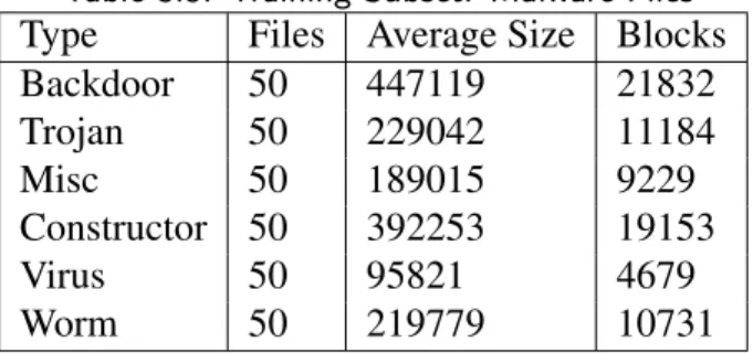
Kolter and Maloof [2] performed further research to determine whether a malicious file could be classified based on its payload function. Since many executables perform multiple functions (e.g. a payload could be a backdoor and keylogger) the authors chose one-versus-allclassification, grouping all of the executables with a particular functionality into a class and all others into a non-class. They applied classification to all the models and reported combined positive results. For example, a file could be classified as a backdoor according to one model and a keylogger according to another. Again, boosted J48 decision trees produced the highest AUCs: .88 for mass mail payloads, .87 for backdoor, and .91 for viruses at 95% confidence intervals. Unlike other studies, Kolter and Maloof implemented the system in a real-world, online application and measured the false-positive rates on 291 new, previously unseen executables as shown Table 2.3. Although the performance of the

Table 2.2: Kolter and Maloof: PE Classification with Top 500 N-grams Length 4, after [2, p. 2731] Method AUC Boosted J48 .9958+/-.0024 SVM .9925+/-.0033 Boosted SVM .9903+/-.0038 IBk, k=5 .9899+/-.0038

Boosted Naïve Bayes .9887+/-.0042

J48 .9712+/-.0067

system decreased, boosted decision trees yielded less than 10% false positive rates 100% of the time. Overall, the authors conclude that J48 boosted decision trees are highly effective with 4-gram byte distributions for determining maliciousness and, to a moderate extent, payload. However, the results apply only to PE executables and a small subset of possible payload classifications.

2.2

File Type Classification

Similar to malware detection, a number of studies have examined the use of machine learn-ing techniques for file fragment classification.

Li and Stolfo, as cited above [3], used the unigram byte histograms of head and tail sectors for eight file types and applied single centroid, k-nearest neighbor clustering, and centroids with exemplar files to develop models of each type. They achieved superior results for file type identification (see Table 2.4), as opposed to their malware experiments. The highest performing method compared the unigram distributions of test files (a subset consisting of 1 in 5 randomly selected files without replacement) to the remaining training files using Manhattan distance. However, this technique has several limitations for our purposes; it relies on header information that is often not available in forensic practice and provides the type of an entire file. It does not necessarily extend to file fragment identification. It is also largely dependent on file type signatures found in the head and tail, making it easy for attackers to evade.

Calhoun and Coles [12] considered four file types (jpg, bmp, gif, andpdf). They used linear discriminant analysis with nine statistical variations of entropy and longest common substring. The algorithm finds linear combinations of features to draw classification lines in pairwise comparisons; e.g.jpgvs.bmpandbmpvs. gif. The best discriminant relied on ASCII code frequencies (0x32-0x192), low byte frequencies (<0x32), high byte (>0x32) frequencies, the sum of the four highest byte frequencies, and the standard deviation of the frequencies with 128 bytes of header removed and 1024 byte blocks. It yielded an average accuracy of 88.3% across all four types. They found that different combinations of features and pairs produced better results than other combinations. For example,jpgandbmpfiles could be distinguished with 100% accuracy using a combination of all possible features. Interestingly, the best overall discriminant did not include entropy. Veenman [13] also used linear discriminant analysis but expanded the study to 11 file types with Shannon entropy

Table 2.3: Kolter and Maloof: PE Classification of 291 Unseen Samples, after [2, p. 2735]

Method FP = .01 FP =.05 FP=.1

Predicted/Actual Predicted/Actual Predicted/Actual

Boosted J48 .94 / .86 .99 / .98 1.00 / 1.00

SVM .82 / .98 .98 / .90 .99 / .93

Boosted SVM .86 / .56 .98 / .89 .99 / . 92

IBK, k = 5 .90 /.67 .99 / .81 1.00 / .99

Boosted Naïve Bayes .79 / .55 .94 / .93 .98 /.98

J48 .20 / .34 .97 / .94 .98 / .95

Naïve Bayes .48 / .28 .57 / .72 .81 / .83

Table 2.4: Li and Stolfo: Fileprint Results, after [3, p. 70]

Experiment EXE GIF JPG PDF DOC Average

Single-centroid 88.3% 62.7% 84% 68.3% 88.3% 82%

Multi-centroid 88.9% 76.8% 85.7% 92.3% 94.5% 89.5%

Exemplar files 94.1% 93.9% 77.1% 95.3% 98.9% 93.8%

and Kolmogorov complexity as features. He analyzed 4096 byte blocks. His experiments were accurate 45% of the time across the 11 types and found similarly that some types are more easily classified than others.

Axelsson [14] considered a larger set of file fragment types and again found that fragments, especially those with high entropy, were not easily classified even with a different learning method. Axelsson used k-nearest neighbors clustering with compression distance, 10 trials, 10 random test files, and 14 random 512 byte blocks from each, against 3,000 fragments of known types. Of the 28 file types considered,Javafragments were most easily classified, though at a disappointing accuracy of 48%. On average, accuracy was 34%.

Conti et al. [15] achieved better results using Shannon entropy, Hamming weight, Chi-square goodness of fit, and mean byte value features grouped by k-nearest neighbor with Euclidean distance. Their study boasts accuracy rates ranging from 88% to 100% depend-ing on type. This is especially impressive given the source of the data which included text, encoded fragments, machine code, and bitmap fragments gathered through various sources or constructed from existing files. The data sources, however, were somewhat contrived and the technique did not perform well on actual file fragments.

During the time that the experiments in this paper were conducted, another study was pub-lished that tested combinations of features used in over twenty different file fragment clas-sification studies. It is by far the most comprehensive study to-date. Using a newly con-structed (and distributable) dataset with 38 file types, Nicole Beebe et al. achieved 73.4% classification accuracy across all types. They used support vector machine and varied in-put features to include unigrams and bigrams, complexity, and other byte frequency-based measures [16]. The publication provides a rather comprehensive summary of features used across recent experiments. Beebe concludes that the most performant approach is to use concatenated unigrams and bigrams with linear SVM. An open source tool called

Sceadan[17], implements their approach. It is available online along with their dataset.

2.3

Summary

This chapter familiarized the reader with a variety of recent machine learning approaches including variations on learning algorithms, input features, and data sources applied to malware classification and fragment identification. The limited success of string and sig-nature based approaches lead us to consider novel methods that employ statistical charac-teristics of byte content. The following chapters describe our methods for evaluating the information-theoretic based methods asserted by Tabish et al. [4] for malware classification tasks and NLP inspired approach employed by Fitzgerald et al. for file type classification tasks [5].

CHAPTER 3:

Methodologies

In this chapter, we describe the methods we used to conduct malware and file fragment machine learning experiments. First, we describe our data sources and attempts to obtain the training and testing sets used by Tabish [4] and Fitzgerald c [5] for replication pur-poses. We define the features used in our experiments as well as learning algorithms and parameters. This chapter describes the procedures and tools we use to perform malware classification and preliminary file type tests.

3.1

Datasets

This section describes the repositories used in our experiments including their provenance and summary statistics. The following sections explain how data was selected.

For file fragment identification tasks, we required a repository containing a range of file types commonly found on hard drives and in other media of forensic interest. The

govdocs1corpus by Garfinkel et al. [18] is a rich database with a million files and over 50

different file types. It is the main dataset used in Fitzgerald et al.’s experiments. Unfortu-nately, we were unable to obtain a precise list of the files used by Fitzgerald [5]. In a best effort attempt to remain as true as possible to Fitzgerald’s procedures, we obtained a local version of thegovdocs1repository and examine the same extensions as those presented in Fitzgerald’s 2012 paper [5].

To reproduce information-theoretic feature experiments on malware we needed a set of be-nign files and malware files of known type, matching those used by Tabish et al.Govdocs1

provided benignpdf, jpg, anddocfiles. We obtainedexe, zip, andmp3files by mining open-source internet repositories and lab computers. The provenance of these files is de-scribed later in this section. It should be noted that the six benign types used by Tabish et al. are common candidates for attackers attempting to obfuscate malicious code in docu-ments, email attachdocu-ments, and internet downloads. The list of good candidates, of course, is not limited to these six. Like Tabish et al. [4] we utilize the VXHeavens[19] malware database, a large sample of malicious files created by a range of novice to professional hackers discovered on the internet over the past several years. We were, again, unable to

obtain the precise files used in the original studies, but replicate the experiments as closely as possible.

3.1.1

VXHeavens

Corpus

Until March, 2012 VXHeavens was a freely available collection maintained by a user named Herm1t at vx.netlux.org [19]. Its self-proclaimed goal was to provide expert level information and education about computer viruses. The web server was seized by Ukrainian police and Herm1t was prosecuted in March 2012 to intent the share and sell malicious code. It was one of the few existing, public malware repositories and has been used in a number of academic studies including Tabish et al.’s work [4] [20] - [22] to cite a few. After completing the experiments in this study,VXHeavenscame back online. It can be accessed atwww.vxheavens.org.

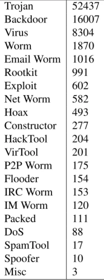
As recommended byVXHeavens’s splash page at the time this study was conducted [23], we sourced our version from The Pirate Bay [24]. The torrent and peer-to-peer download completed on February 21, 2013 delivering 44GB of data and 83,852 files. While there are no official sources to determine provenance for the individual specimens, our review of the files along with VXHeavensrelated blog posts, articles, and other web media suggest that the VXHeavens repository is one of the largest collections available, that it contains samples collected over the last decade and likely represents viruses less complex than those produced by nation states and parties with capital resources. Since these experiments, the webpage has been restored and it appears that new owners are crowd sourcing and maintaining an expanded 400GB database. As addressed more thoroughly at the end of this paper, experimenting with newVXHeavens samples posted since our 2013 download remains future work. Many of the files in the 44GB VXHeavens download used in this study are included in industry alerting databases such as Microsoft’s Security Essential’s and Symantec’s Virus Definition databases [25]. Each file is classified by the its malicious function and the target operating system. A count of each type is shown in Table 3.1 and by the type of operating system the file runs on (e.g. Win32, DOS). The majority, 75,530 files, are Win32 PE format.

3.1.2

Govdocs Digital Corpus

The govdocs1digital corpora includes one million files that were obtained by searching

Table 3.1: Counts for each File Type in theVXHeavensCorpus Label Count Trojan 52437 Backdoor 16007 Virus 8304 Worm 1870 Email Worm 1016 Rootkit 991 Exploit 602 Net Worm 582 Hoax 493 Constructor 277 HackTool 204 VirTool 201 P2P Worm 175 Flooder 154 IRC Worm 153 IM Worm 120 Packed 111 DoS 88 SpamTool 17 Spoofer 10 Misc 3

random numbers between 1 and 1 million [18]. The files have been reviewed to determine proper extension, but this is an ongoing and imperfect process. As stated in thegovdocs1

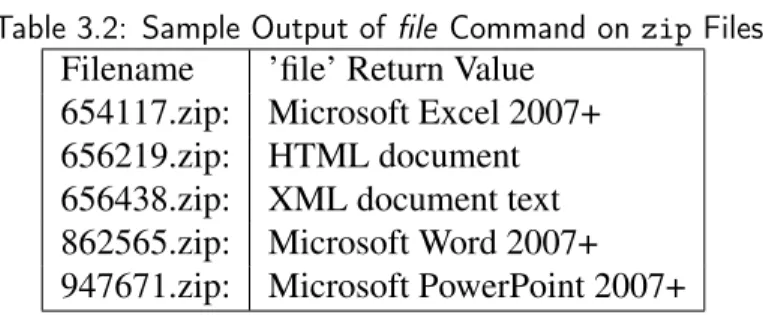
documentation [18], the listed extension is not a precise indicator of actual file type. Ta-ble 3.3 shows the estimates provided by thegovdocs1documentation for the database. We explored alternative methods for identifying the actual file type, but doing this task correctly over a large dataset is beyond the scope of this study. One alternative relies onlibmagic

descriptions instead of the file extension to establish ground truth. Unfortunately, similar challenges exist with both methods. Many files can be classified as more than one type while others are reported as “unknown”. For example, csvfiles are essentially txtfiles except that content is separated by strategically placed commas. New versions of Windows Office files are similar toxlsx. Pptxfiles are similar tozipfiles. Table 3.2 shows a por-tion of the output from running thefilecommand onzipfiles ingovdocs1. A variety of types were returned.

Table 3.2: Sample Output offile Command onzipFiles

Filename ’file’ Return Value 654117.zip: Microsoft Excel 2007+

656219.zip: HTML document

656438.zip: XML document text 862565.zip: Microsoft Word 2007+ 947671.zip: Microsoft PowerPoint 2007+

File extension inaccuracies with respect to ground truth are potential sources of noise in training, testing, and the final results.

3.1.3

Supplemental Benign Files

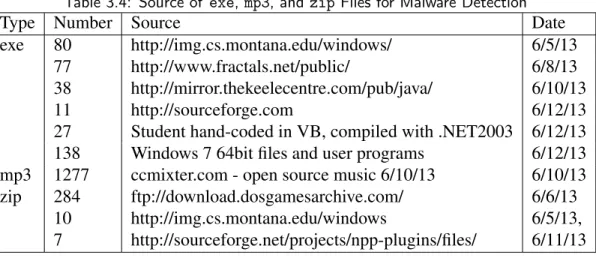
For the malware detection experiments we required a benign dataset that matched Tabish et al.’s set containing six types. Three of these types were not available ingovdocs1. These exceptions are shown in Table 3.4. We obtained the needed types by mining websites that host open-source collections as well as lab computer drives. In this section we summarize the sources forexe,mp3, andzipfiles in the benign dataset issued in our malware detection experiments. The dataset is available upon request.

3.1.4

Data Selection

Malware Files

Following Tabish et al. [4], we focus on six malware categories found in the VXHeavens

collection. We examined samples and describe what is included in each category: Backdoor

A backdoor is a program that listens for commands over a network connection and gives an attacker remote control of a system. Backdoors typically require client/server components to accomplish the network communication portion. Most backdoors allow an attacker to perform file transfers, acquire passwords, and execute commands. More nefarious versions

Table 3.3: Govdocs Extension Accuracy Estimates

Accuracy Rating Percentage

High 92.5%

Medium 7.0%

Low <.25%

Table 3.4: Source of exe,mp3, and zip Files for Malware Detection

Type Number Source Date

exe 80 http://img.cs.montana.edu/windows/ 6/5/13

77 http://www.fractals.net/public/ 6/8/13

38 http://mirror.thekeelecentre.com/pub/java/ 6/10/13

11 http://sourceforge.com 6/12/13

27 Student hand-coded in VB, compiled with .NET2003 6/12/13

138 Windows 7 64bit files and user programs 6/12/13

mp3 1277 ccmixter.com - open source music 6/10/13 6/10/13

zip 284 ftp://download.dosgamesarchive.com/ 6/6/13

10 http://img.cs.montana.edu/windows 6/5/13,

7 http://sourceforge.net/projects/npp-plugins/files/ 6/11/13

includebotswhich automatically cause the infected system to attack other systems.

Zom-bies, bots andagents are typically used to carry out coordinated DDOS attacks. RATs or

remote administration tools allow the attacker to access the system as needed, granting

control over the systems devices (webcams, microphones, and speakers). BACKDOOR EXAMPLE:

Rbot is a family of backdoor that allows the attacker to take control of a victim’s machine. Rbot connects to an IRC server where it receives commands from at-tackers. For example, the attacker may run commands that scan the infected com-puter’s network for exploitable windows vulnerabilities, look for file shares with weak passwords, infect other computers on the network, and launch denial of ser-vice attacks. [26]

Trojan

Trojans are programs that appear benign but perform covert, malicious activity. Trojans come in variety of forms. Some trojans completely replace an existing program but main-tain its functionality, while others simply modify or add additional functions to existing programs. A generic example would be a login program that illegally collects and transmits passwords. Trojans can cause serious technical issues ranging from performance disruption to making the system unusable.

Trojan.Win32.Buzus is a program that installs unauthorized files on the infected system, typically a worm, capable of spreading via removable USB drives and per-forming other unwarranted actions on the system. It is typically distributed as an executable file attached to an e-mail message or downloaded from a compromised website. [27]

Virus

Viruses are designed to self-replicate and distribute themselves to other files, programs, or computers. Viruses are often inserted into a benign carrier. For example, a word document might contain a viral macro. A virus that runs inside or is executed by another application is an interpreted virus. Somecompiled viruses are stand-alone files that can be directly executed by the operating system. Virus impacts range from causing moderately annoying pop-ups to overtly malicious modification, dissemination, or destruction of sensitive data. VIRUS EXAMPLE:

Virus.WWin32.Xorera family of file infectors. The virus waits for a certain amount

of time to pass between infecting more files. According Microsoft’s repository, it en-crypts and prepends the virus code to an existing document. It has worm capabilities and is able to drop copies of items in writable drives, as well as rootkit capabilities which allow it to avoid detection. It is a virus that can infect both files and boot sectors. [28]

Worm

Worms are self-replicating, self-propagating, stand-alone programs that can execute with-out user intervention. Network worms take advantage of network services to infect other systems. One common medium by which a worm spreads is via mass email. The process can overwhelm email services and cause performance issues for infected systems. Worms are also used to call backdoors, perform general denial of service attacks, and aid other types of attacks.

WORM EXAMPLE:

Worm.Win32.Autorunis a family of worms that secretly copies itself into programs

time the the host program is run. [29] Constructor

Constructors are malware creation toolkits that allow users to specify settings and automat-ically assemble new code. They are useful for attackers with little programming experience and for creating polymorphic code [30]. The kits range from simple to very sophisticated in terms of the options and features they provide.

CONSTRUCTOR EXAMPLE:

Constructor.Win32.NGVCK.0_40is a variant ofProgram:Win32/Advdown.Athat

downloads malware from http://www.paragon-software.com/ and mainly targets computers in Nepal, Moldova, Togo, Somalia, and Vietnam. [31]

Miscellaneous

The misccategory includes exploits, flooders, hacktools, virtools, and hoaxes. Exploits, hacktools, and virtools are programs that take advantage of vulnerabilities, such as causing buffer overflow so the attacker gains execution control. Flooders run mass email, instant messaging, and SMS attacks. Hoaxes are non-malicious alerts and programs that cause damage through social engineering. Hoaxes can cause a backlog of complaints to IT de-partments or trick users into making changes to security settings that are less secure. Selection: Malware and Benign Files for Training and Testing

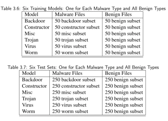
Tabish et al. built six separate classifiers, one for each category of malware using 50 random files of the specific type of malware (see Table 3.5) and a total of 50 random benigndoc,

jpg,exe,pdf,zip, andmp3files. They do not specify how many of each benign type were represented. Tabish et al. claim to test their models on all remaining files which would seem to include the entireVXHeavensdatabase and approximately 295 files of each benign type. Since Tabish et al. were unable to provide their precise dataset upon request, we chose to test the types equally. Ultimately, we collected a subset of 300 files for each of the following types: virus, trojan, worm, constructor, backdoor, misc, exe, zip, mp3, doc, pdf, and

jpg. Following the cited method, we created six training sets, one for each malware type. Each training set is comprised of blocks from 100 files including 50 randomly selected malware files of the type in question and 50 total benign files (8-9 of each type). Table 3.6 summarizes the composition of the six training models, one for each malware type, used

in our classification experiments. Likewise, we create six test sets each containing the remaining 250 malware files of the particular type and 250 benign files (41-42 of each benign type), so that files used in training are excluded from testing. A summary of the test files is given in Table 3.7. It is important that no training files are used in testing since one of our goals is to verify whether the Tabish method is effective on unseen files.

File Fragment Identification

Like Fitzgerald et al. we source from thegovdocs1corpus to obtain a variety of file types. There are 50 different extensions represented in the repository and Fitzgerald et al. study 24 of them. This study examines the 23 extensions highlighted in Table 3.8. The frequency of types across thegovdocs1corpus is not uniform. Following Fitzgerald, our study excludes uncommon extensions that are not of interest as well as those where the sample is not large enough to ensure separate training and testing. One of such types is.zipfiles. Although Fitzgerald et al. cite 10zipfiles in thegovdocs1database, we discovered that these files are not actually zip files. Therefore the govdocs1 repository does not have sufficient representation ofzipfiles and we have decided to exclude them from all our trials. In the fashion of Fitzgerald’s work, this study assumes that extension is ground truth for a file’s type even though this method can produce inaccuracies.

From the list of almost 1,000,000 files in the the govdocs1repository, we randomly se-lected sets of 1,000, 2,000, and 4,000 blocks of 1,204 bytes from each of the 23 types excluding file header and footer blocks. We exclude header and footer blocks because these sections often contain descriptive flags that make identification too easy. It is prefer-able to represent a variety of different sample files for each type so that the model is not overtrained to a particular file. We also ensure that the training and testing datasets are comprised of blocks from mutually exclusive files even though other papers do not appear

Table 3.5: Training Subset: Malware Files

Type Files Average Size Blocks

Backdoor 50 447119 21832 Trojan 50 229042 11184 Misc 50 189015 9229 Constructor 50 392253 19153 Virus 50 95821 4679 Worm 50 219779 10731

Table 3.6: Six Training Models: One for Each Malware Type and All Benign Types

Model Malware Files Benign Files

Backdoor 50 backdoor subset 50 benign subset Constructor 50 constructor subset 50 benign subset

Misc 50 misc subset 50 benign subset

Trojan 50 trojan subset 50 benign subset

Virus 50 virus subset 50 benign subset

Worm 50 worm subset 50 benign subset

Table 3.7: Six Test Sets: One for Each Malware Type and All Benign Types

Model Malware Files Benign Files

Backdoor 250 backdoor subset 250 benign subset Constructor 250 constructor subset 250 benign subset

Misc 250 misc subset 250 benign subset

Trojan 250 trojan subset 250 benign subset

Virus 250 virus subset 250 benign subset

Worm 250 worm subset 250 benign subset

concerned about this. We applied the following methodology to ensure sufficient represen-tation of each type from a variety of files and that there is no overlap in training and testing data.

First, we randomly selected 1,000, 2,000 and 4,000 files of each type assuming random ordering of the file list. We then randomly selected one 1,024 byte block from each file without replacement of blocks until there were 1,000, 2,000 or 4,000 blocks per file type. For types where there were less than 1,000, 2,000 or 4,000 distinct files, some files are revisited and another random block is selected from the file. We call this anlimiteddataset: each block comes from a distinct file. Put differently, there is a 1:1 block-to-file ratio. The types of files represented in the limited dataset are shown in Table 3.10. The unlimited

dataset includes subsets of 1,000, 2,000 and 4,000 blocks per type but excludes types with-out enough files to achieve a 1:1 block-to-file ratio. See Table 3.9 for a summary. For the unlimited sets that included all types, we divided each 1,000, 2,000 and 4,000 block pool into 2 pools to obtain a 9:1 training-to-testing ratio. To prevent any overlap between training and testing files in the limited set, we ignore any blocks remaining at the end of a file after building the training set. We start building the test set from a new, unused file in the pool. Note that, for these types, there is not a perfect 9:1 ratio. In the limited sets, files

Table 3.8: Govdocs1File Types Used in Fragment Experiments Highlighted

Extension Count of files MB

pdf 232794 127492 html 191407 11222 **jpg 109278 35970 *text 83805 50406 doc 80648 30099 xls 66599 29041 ppt 50257 122918 xml 41994 8405 gif 36301 2920 ps 22129 27668 csv 18396 3347 gz 13870 8651 log 10241 4204 unknown 8188 4456 eps 5465 3082 png 4125 1079 swf 3691 1853 pps 1629 3629 kml 995 149 kmz 949 226 hlp 660 5 sql 632 226 dwf 474 42 java 323 11 *txt 286 9 pptx 219 562 tmp 196 15 docx 169 32 ttf 104 1 js 92 2 pub 76 1 bmp 75 31 xbm 51 1 xlsx 46 6 jar 34 2 zip 27 1 wp 17 2 sys 8 0 dll 7 0 exe 5 0 exported 5 0 **jpeg 3 0 tif 3 0 chp 2 0 data 1 0 pst 1 0 squeak 1 12 Total 986278 477641 *types can be collapsed

represented in training were necessarily distinct from the files represented in testing. This guarantee allowed us to use Orange’s [32] built in cross-validation. The experiments are described further in the next section. In total, our process yielded six datasets as shown in Table 3.9 and Table 3.10.

3.2

Feature Generation

This section defines the features extracted from malware and benign files, including the so-called information-theoretic features used by Tabish [4] and so-so-called NLP features used by Fitzgerald [5]. Although their naming is somewhat specious, we have chosen to adopt the authors’ original terminology for simplicity throughout this paper. The features dis-cussed in this section were extracted for each block in the testing and training datasets. We

Table 3.9: File Type Classification on Unlimited Dataset: Blocks Come From Distinct Files

Blocks Total Included types

per type types (distinct original files)

1000 16 jpg gz png ppt doc pdf txt html xml xls gif ps csv swf pps rtf

2000 14 jpg gz png ppt doc pdf txt html xml xls gif ps csv swf

4000 13 jpg gz png ppt doc pdf txt html xml xls gif ps csv

Table 3.10: File Type Classification Limited Dataset: Blocks Can Come From Repeat Files

Blocks Total Under-represented types per type types (repeat original files)

1000 23 (all) pptx docx xlsx sql java tex bmp

2000 23 (all) pptx docx xlsx rtf pps sql java tex bmp

4000 23 (all) swf pptx docx xlsx rtf pps sql java tex bmp

performed experiments using different combinations of selected features to determine the features with highest accuracy and lowest false positive rate.

3.2.1

Information-Theoretic Features

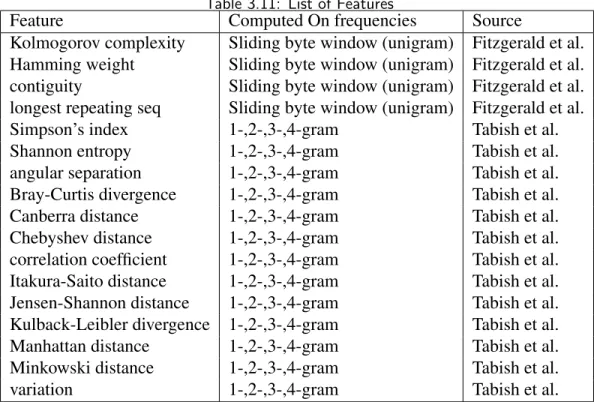
Information theory provides mathematical methods for quantifying information such as the limits on data compression, reliable transmission, and data storage [33]. Note that information theory is not concerned with the semantic meaning or function of the data. Instead, it describes numeric qualities of the data. Table 3.11 summarizes the features we compute and the previous studies that motivated us to include them.

Some of the features are based on common information-theoretic measures computer sci-ence, biology, ecology, and other statistical sciences. A subset of these features are more commonly used for language processing tasks. Several so-called NLP features are used in Fitzgerald’s study, and therefore, in our experiments as well. In total, we include 17 distinct information-theoretic features. The features used in Tabish’s malware study [4] are computed for 1-, 2-, 3-, and 4-gram frequency distributions. Following Fitzgerald’s example [5], these include NLP features on per block unigram frequencies (count of byte values 0-256). We experiment with combinations proposed by both authors and various combinations of features. Experiments are described in Section 3.4.

Following Tabish et al.’s work [4], we adopt their terminology to reference the statistical features they present, but we recognize that it is somewhat an abuse of notation to say we

Table 3.11: List of Features

Feature Computed On frequencies Source

Kolmogorov complexity Sliding byte window (unigram) Fitzgerald et al.

Hamming weight Sliding byte window (unigram) Fitzgerald et al.

contiguity Sliding byte window (unigram) Fitzgerald et al.

longest repeating seq Sliding byte window (unigram) Fitzgerald et al.

Simpson’s index 1-,2-,3-,4-gram Tabish et al.

Shannon entropy 1-,2-,3-,4-gram Tabish et al.

angular separation 1-,2-,3-,4-gram Tabish et al.

Bray-Curtis divergence 1-,2-,3-,4-gram Tabish et al.

Canberra distance 1-,2-,3-,4-gram Tabish et al.

Chebyshev distance 1-,2-,3-,4-gram Tabish et al.

correlation coefficient 1-,2-,3-,4-gram Tabish et al.

Itakura-Saito distance 1-,2-,3-,4-gram Tabish et al.

Jensen-Shannon distance 1-,2-,3-,4-gram Tabish et al.

Kulback-Leibler divergence 1-,2-,3-,4-gram Tabish et al.

Manhattan distance 1-,2-,3-,4-gram Tabish et al.

Minkowski distance 1-,2-,3-,4-gram Tabish et al.

variation 1-,2-,3-,4-gram Tabish et al.

apply “information-theoretic formulas”. We simply take advantage of the fact that these measures produce a numeric description that may prove useful in identifying and classify-ing the information encoded in each block. Typically, information-theoretic distance and divergence metrics are used to observe the difference between two points or input vectors, for example, the difference between a two vectors representing prior and actual probability distributions. This study applies information-theoretic formulas on two input vectors, but unlike typical applications, our vectors are derived from the same frequency distribution. We denote the first vector as Xi. It represents the left end of each n-gram frequency

distribution such that Xi = (X0,X1, . . . ,Xn−2),n=28x, andxis then−gramsizein bytes.

For example, if x=1 byte, the first frequency distribution counts the occurrences of n-gram values in range (0,1,2, . . . ,254) for each block. The second vector X_i+1 is the same distribution shifted by 1. It represents the right end of the frequency curve such that X_i+1 = (X1,X2, . . . ,Xn−1),n =28x. If x = 1 byte again, Xi+1 counts the frequency

of n-grams whose values range from (1,2,3, . . . ,255). We reflect the fact that the fea-ture generation methods are somewhat contrived with respect to their typical

information-theoretic uses, by representing the feature formulas with prime (’) and the input vectors as

XiandXi+1rather than pandq.

Ultimately, the goal of applying features based on information theory is to produce a quan-titative profile of the binary information contained in each file. Even if those measurements do not have clear mathematical meaning, they may have be useful descriptors and provide an identifiable signal. The selected features are defined as follows:

Minkowski Distance

The Minkowski distance gives the m-order distance or the power mean of the component-wise differences between two points or vectors. It is a generalization of Manhattan distance and Euclidean distance.

Minkowski(p,q) = n

∑

∑

The Chebyshev distance is the maximum distance between two vectors along any coordi-nate system. In other words, it is the limit of the Minkowski distance asmgoes to infinity.

Chebyshev(p,q) = lim k→∞ n

∑

The Manhattan distance is the geometric, right angle distance between two points in vector space given a Cartesian coordinate system. It is computed by taking the sum of line segment lengths between points along coordinate axes. It is an instance of the Minkowski distance wherem=1.

Manhattan(p,q) = n

∑

∑

Canberra distance is a weighted version of the Manhattan distance. Typically it is used to find the normalized distance between two points (p,q)in vector space. For example, in intrusion detection Canberra distance might be used to quantify how similar a suspect file is to a predetermined, normal model.

Canberra(p,q) = n

∑

∑

Bray Curtis Distance

The Bray Curtis distance is a measure of dissimilarity between two frequency distributions. It is commonly used in ecology to measure the difference between compositions of species at two sites. It can also be considered a normalized Manhattan distance.

BrayCurtis(p,q) = ∑ n i=1|pi−qi| ∑ni=1(pi+qi) (3.9) BrayCurtis0(Xi,Xi+1) = ∑ n i=1|Xi−Xi+1| ∑n_i=1(Xi+Xi+1) (3.10) Angular Separation

Angular separation is a similarity measure based on the cosine of the angle between two vectors. High angular separation means that the input vectors are similar.

AngularSep(p,q) = n−1 ∑ i=0 (p_i)(q_i) s n−1 ∑ i=0 (p_i)2n_∑−1 i=0 (qi)2 (3.11) AngularSep0(Xi,Xi+1) = n−1 ∑ i=0 (X_i)(X_i+1) s n−1 ∑ i=0 (Xi)2 n−1 ∑ i=0 (Xi+1)2 (3.12) Correlation Coefficient

Correlation coefficient is the separation between vectors centered around the mean of the vector coordinates. A high correlation coefficient implies similarity.

CorrCoe f f(p,q) = n ∑ i=1 (pi−p)(q¯ i−q)¯ r _n ∑ i=1 (p_i−p)¯ 2 _∑n i=1 (q_i−q)¯ 2 (3.13) CorrCoe f0(Xi,Xi+1) = n−1 ∑ i=0 (X_i−_X¯_i)(Xi+1−X¯_i+1) s n−1 ∑ i=0 (Xi−X¯i)2 n−1 ∑ i=0 (Xi+1−X¯i+1)2 (3.14) Shannon Entropy

Shannon entropy is a measure of how much information is contained in a message or how much information is missing if a symbol in a message is unknown. Entropy quantifies the dispersal of a distribution and the uncertainty of a random variable.

Entropy(X) =−

n

∑

i=1

p(xi)log2p(xi) (3.15)

Entropy0(X) =−

n

∑

i=0

p(xi)log2p(xi) (3.16)

where p(xi)is the probability of theithn-gram in a block.

Total Variation

In probability, total variation is the largest possible distance between two distributions for a given event. It is related to the Kolmogorov-Smirnov test [34] which measures the distance between an empirical and cumulative distribution for a sample.

Variation(p,q) = 1 2

∑

∑

Kullback-Leibler divergence [35] measures how much information is lost by trying to ap-proximate one distribution with another. It is often used to encode and quantify how far a model or theory is from a true distribution and is the basis for information gain calculations used in decision tree induction.

KullLeib(pkq) = n

∑

∑

Jensen-Shannon divergence [36] is a symmetric, smoothed version of Kullback-Leibler divergence. It measures similarity between probability distributions.

JenShan(pkq) = 1

2K(pkm) + 1

wherem= 1₂(p+q). JenShan0(XikXi+1) = 1 2D(XikM) + 1 2D(Xi+1kM) (3.22) whereM= 1₂(Xi+Xi+1). Itakura-Saito Distance

Itakura-Saito distance [37] is an example of Bregman divergence, a generalized Euclidean Distance that maintains certain convexity, non-negativity, and duality properties.

ItakSaito(p,q) = n

∑

∑

Simpson’s index [38] is commonly used in ecology to determine the probability that two specimens selected at random from an ecosystem will belong to the same class. The vari-ablenrepresents the number of organisms of a particular class andN is the total count of all organisms. For binary file information,nis the count of each possible n-gram value and

N is the total number of n-grams in a block.

Simpsons=∑ n i=0n(n−1) N(N−1) (3.25) Simpsons0=∑ k i=0nk(nk−1) N(N−1) (3.26)

wheren_k is the frequency of thekth value andN is the number ofn-grams in a block.

3.2.2

Natural Language Processing Features

The following features are used by Fitzgerald et al. [5] to distinguish file fragments. Fol-lowing Fitzgerald et al., we apply them in our file fragment identification experiments. We also include them in some of our malware detection trials with promising results. While the measures described in this section are common in language processing tasks, they do

not strictly belong to that domain of problems. We adopt Fitzgerald’s notation throughout this paper.

Contiguity

Contiguity measures the average distance between byte sequences. Essentially, it is a heuristic that can potentially determine if there is a general, repeating pattern to the data. In this study we only compute the contiguity between consecutive 1-byte n-grams, but in future research it might prove useful to explore other pattern lengths. When computing different n-gram lengths, it will also be necessary to consider the various offsets at which a pattern might start. For feature generation, we define contiguity as:

Contiguity= k−1

∑

wherekis the block size in bytes.

Hamming Weight

Hamming weight is computed by summing the 1s and dividing by the total number of bits in a binary string. For a given string, it is the same as the Hamming distance from the all-zero string of equal length.

HammingWeight= k

∑

wherekis the block size in bytes.

Longest Repeating Sequence Length

Some files contain long strings of a repeated byte sequence. Empty document files, for example, contain long strings of 0s. This measure is computed as the length of the longest repetition of any single byte value. It is also possible to take the string made up of any single repeating n-gram value. For simplicity, we observed only the longest string with respect to bytes.

LongRep=max

i length(si) (3.29)

Kolmogorov Complexity

The Kolmogorov complexity, also known as algorithmic complexity, is the length of the shortest descriptor or language needed to produce a string. It can be approximated using compression algorithms likebzipandgzip. We apply Python’s zlibcompression function to obtain an estimate.

Kolmogorov(s) =|d(s)| (3.30)

whered(s)is the shortest descriptor ofs.

3.3

Learning Algorithms

This section is a review of the learning algorithms used in each experiment. Each algorithm was applied to the training sets to obtain a classifier. Each classifier was then evaluated on the test sets previously described.

3.3.1

k-Nearest Neighbor (KNN)

KNN is an instance-based learning method that classifies objects by taking a majority vote among its neighbors. The training examples are represented as vectors in a multidimen-sional space and their ground truth classes are known. The user defines a positive constant integerk which is the number of neighbors that will be allowed to vote. A distance such as Euclidean distance or Hamming distance determines thek closest neighbors in the fea-ture space to the object in question. The new object is labeled with the class that is most common amongst the neighbors. This is disadvantageous when the data is skewed. For example, a class may dominate the feature space if there is a disproportionate number of examples of that class to other classes.

Several parameter optimizations have been proposed to improve the performance of KNN learners. One method is to weight neighbors by their distance to the new point. It may also be productive to explore the optimal value for k. This is important because ak that is too large will not be able to distinguish the classes. Another method is to vary the distance metric used to determine nearest neighbors. Scaling and dimension reduction are often utilized to reduce noise and eliminate irrelevant features. Some studies use genetic algorithms in preprocessing to determine the optimal parameter values.

3.3.2

Decision Trees

Decision trees are an inductive method that create a list of parameters from a set of fea-tures and training data, and classify a new file based on those parameters. Following its name, combinations of parameters can be represented as branches on a tree. Classes are represented as tree leaves. There are a number of decision tree algorithms for generating rules from the training data. The algorithms vary in terms of what measure is used to split data, whether the predicted class is continuous or discrete, how over-fitting is handled, and whether missing values are permitted. The most common are C4.5, its ancestor ID3 [39], and the Weka implementation of J48.

For this study, decision trees are implemented with Python Orange’sorange.TreeLearner

module, which uses a top-down induction method similar to C4.5. By default, Orange [40] uses the information gain ratio (information gain divided by