Skills, Partnerships and Tenancy in Sri Lankan Rice Farms

ECONOMIC GROWTH CENTER

YALE UNIVERSITY

P.O. Box 208269

New Haven, Connecticut 06520-8269

http://www.econ.yale.edu/~egcenter/

CENTER DISCUSSION PAPER NO. 819

SKILLS, PARTNERSHIP AND TENANCY

IN SRI LANKAN RICE FARMS

Sanjaya DeSilva

Bard College

October 2000

Note: Center Discussion Papers are preliminary materials circulated to stimulate discussions and critical comments.

Financial support was provided by the Ford Foundation and the Economic Growth Center at Yale

University.

I am thankful to Robert E. Evenson, T.N. Srinivasan, Christopher Udry and Jean O. Lanjouw for

their invaluable comments and suggestions. Versions of this paper were presented at the Northeast

Universities Development Consortium (NEUDC) Conferences 1998 and 2000 and various

workshops at Yale. I gratefully acknowledge the Department of Census and Statistics in Sri Lanka

for granting access to their data. Please send comments and suggestions to desilva@bard.edu.

ABSTRACT

This paper examines whether sharecroppers and fixed-rent tenants in the rice farms of South Asia are distinguished by their farming skills. The idea that fixed-rent contracts are typically given to relatively skilled tenants dates back to the agricultural (tenancy) ladder hypothesis of Spillman [1919]. The screening models [e.g. Hallagan 1978] that have attempted to formalize this idea assume that landlords do not observe the tenants’ skill levels. This assumption is restrictive, and has found little support in empirical studies. The principal-agent model proposed in this paper focuses on the differences between time-intensive and skill-intensive labor tasks. I show that tenancy contracts are designed to match the provision of these tasks with the owners of time and skill inputs. Sharecropping, in this model, provides an incentive scheme that allows for the specialization between a time-abundant tenant and a skill-abundant landlord.

The second part of the paper empirically explores this result with household-level data from Sri Lanka. A two-stage model that distinguishes the choice of contract from the extent of land leased is used. The results clearly show that relatively skilled farmers are more likely to become fixed-rent tenants.I also find that, conditional on contract choice, farming skills do not affect the extent of land leased. A substantial part of the empirical analysis is devoted to the measurement of farming skills. I interpret farming skills as the contribution of observed farmer characteristics to the technical efficiency of the farm. This measure recognizes that many dimensions of skills are observed, and the use of weights computed from a production function to construct the skill index is theoretically more appealing than the ad hoc selection of proxy variables.

KEYWORDS: Land Tenancy, Farming Skills, Agricultural Labor, Sri Lanka

1

The prevalence and persistence of land tenancy contracts have intrigued economists from the days of Adam Smith [1776] and Alfred Marshall [1890]. Although a large and fascinating literature has since evolved on this topic, many important questions on the existence of land tenancy contracts remain unresolved.1 The goal of this paper is to provide a theoretical and empirical answer to one such question, the role of farming skills in the choice between fixed-rent and share-rent contracts.

The idea that skilled farmers obtain fixed-rent contracts dates back to Spillman [1919] who argued that farmers climb an “agricultural ladder” from agricultural labor to share-tenancy and then to fixed-rent tenancy through the gradual acquisition of skills. The ladder hypothesis has important policy implications that are especially relevant to countries, like Sri Lanka, that have attempted to discourage sharecropping through legislation. For example, the model developed in this paper shows that a time scarce landlord will prefer a fixed-rent contract provided that the tenant is sufficiently skilled. Therefore, narrowing the skill gap between landlords and tenants is the key to changing the tenancy mix in favor of fixed-rent farming. Secondly, removing the sharecropping option from the tenancy ladder through legislation leaves agricultural labor as the only option for unskilled tenants. Sharecropping provides a vital link by which unskilled tenants acquire the necessary management skills in partnership with landlords. The empirical estimates show that yields obtained by unskilled sharecroppers if they were to fixed-rent are too low to be feasible.

Over the years, the tenancy ladder has remained largely a “verbal hypothesis”. [Otsuka and Hayami 1993]. The screening model proposed by Hallagan [1978] has attempted to formalize this idea using an adverse selection argument. The critical assumption of this model is that landlords do not observe the entrepreneurial skills of potential tenants. He argues that landlords can choose the contract parameters (share and fixed rents) to induce utility maximizing tenants of different abilities to self-select in

to different types of contracts. Tenants with highest skill levels choose fixed-rent contracts, those with medium-skills self-select into sharecropping and the least skilled ones remain as agricultural laborers. However, the screening model is of limited use because the adverse selection argument falls apart in village economies where social networks are especially strong and information on tenant attributes is easily available.2 This model is also theoretically flawed because it fails to address the landlord’s optimization problem.3

More recent studies of land leasing have emphasized that moral hazard is a greater problem than adverse selection in village economies. The reasons for the severe moral hazard (or agency) problems are twofold: 1) many farm tasks are characterized by long time lags between inputs and the outcome and 2) a variety of random shocks (weather etc.) can make output uncertain and the contribution of workers to output difficult to measure.4 An obvious solution to the moral hazard problem, especially in a modern industrial context, is the direct supervision of workers. However, direct supervision is a directly unproductive activity and can incur heavy costs especially for tasks with the large time lags and greater exposure to production shocks.5 Some examples of such tasks are farm management and decision-making, application of chemicals and fertilizer, irrigation control, seed preparation and care and the supervision of

Bardhan [1984], Bell [1988] and Lanjouw [1999] find that information on the attributes of farmers is widely available in village communities.

3

See Allen [1982] for a discussion of this problem. Allen [1985] attempts to salvage the screening model by looking at the optimization behavior of both parties under the assumption that contracts are designed to prevent default in rent payments. However, he succeeds only in showing that both parties are indifferent between share and fixed rents for certain skill levels. In addition, the advanced payment of a fixed-rent has been shown to be a widely practiced first-best solution for the default problem [Otsuka and Hayami 1993].

4

See Lanjouw [1999] for empirical evidence on the existence of moral hazard problems. 5

short-term workers. 6 Tenancy can be used to allocate these imperfectly marketed labor inputs. Thus, in environments with imperfect factor markets, land tenancy plays a significant economic role by facilitating the efficient allocation of farm inputs.

The differences in the difficulty of supervision across farm tasks are clearly manifested in how these tasks are allocated in a farm’s organization. The easily supervised tasks (harvesting, threshing, weeding etc.) are typically delegated to hired short-term workers or teams of workers who are paid a fixed or piece-rate wage. The more spatially and temporally spread out tasks are, on the other hand, often performed by the owner’s family or tenants.7 The goal of this paper is to understand the mechanism by which some or all of these tasks may be delegated to a tenant.

The motivation for this work comes from several interesting empirical observations made in quite different historical and geographical contexts. The earliest articulation of tenancy as a partnership between a landlord and a tenant comes from a series of papers by Reid [1973, 1975, 1976, 1979] on the emergence of sharecropping as a common form of tenancy in the Post-Bellum American South. He argued that freed slaves possessed large amounts of unskilled labor but lacked the managerial expertise that was required to single-handedly carry out cotton cultivation. The former slaves who lacked management or decision making abilities appear to have formed partnerships with white landlords who, due to their significantly greater experience and resources, possessed these qualities in abundance. Bell and Srinivasan [1985] find similar evidence in the entirely different setting of the contemporary Indian states of Punjab, Bihar and Andhra Pradesh. Their survey questionnaire asked explicit questions about the role landlords and tenants play in making key decisions and performing managerial tasks. The survey

See Bell and Zusman [1976], Bliss and Stern [1982], Pant [1983] and Eswaran and Kotwal [1985a]. Some other tasks, such as harvesting and threshing, are quite amenable to direct supervision. These tasks have outcomes that are immediately and directly observed during a short time frame so that direct monitoring is feasible.

7

In some areas, especially in India, these tasks are sometimes given to permanent hired workers. It has been argued, however, that these permanent workers face very similar incentives to that of family members and are considered a de facto part of the household [Eswaran and Kotwal 1985b].

results show clearly that landlords play a significant role in providing these tasks in sharecropped lands and a minimal role in the fixed-rented farms. Roumasset [1995] reports further evidence of this division of managerial tasks by type of contract. Under Roumasset’s classification, the landlord carries out land and asset management as well as most production decisions, whereas the tenant provides the control of labor and some of the more routine production decisions in sharecropped lands. This mostly anecdotal evidence tells us that sharecropping allows for a skill-abundant landlord and a time-abundant tenant the right incentive schemes to specialize in providing the labor tasks in which they possess a comparative advantage.

Eswaran and Kotwal [1985a], in their seminal theoretical work, focus on two types of skilled labor inputs, management and supervision. They argue that tenancy contracts are designed to offer self-monitoring incentives to the owners of these inputs by tying their incomes to farm output. In this setting, owner-cultivation is chosen if both inputs are provided by the landlord, and a fixed-rent contract is chosen if they are provided entirely by the tenant. Sharecropping provides a solution to the double-incentive problem that arises when both parties provide unenforceable inputs. This is of course a second best solution because of the usual Marshallian inefficiency costs associated with sharing rents. 8

The Eswaran-Kotwal formulation takes the absolute advantage of landlords in management and tenants in supervision as given. The assumption that tenants are somehow endowed with supervisory skills is questionable [Hayami and Otsuka 1993]. To begin with, tenants in share arrangements appear to provide a much broader range of tasks than just supervision. Even if supervision of casual workers is important, it is likely to require very little skill and a large amount of time. Hayami and Otsuka [1993]

Shaban [1987] supports this argument with empirical evidence that yields (controlling for other observed factors) are lower in sharecropped lands. We do not contest this view that sharecropping is less efficient than fixed-rent farming. Our aim is to determine the conditions under which share-tenancy arises in spite of the apparent inefficiencies.

propose that we re-interpret the second input as labor. In this case, a clearer justification must be given as to why tenant may hold an absolute or comparative advantage in providing labor.

In the next section of this paper, we formalize this more general idea by assuming that landlords are time constrained and tenancy is really a solution to a time allocation problem. The two key inputs are skills and time, and they are combined in different proportions to perform each farm activity. We introduce three new features to the standard principal-agent model: 1) tenants are not assumed to have an absolute advantage in any type of skill; 2) landlords are assumed to have time constraints; and 3) landlords are allowed to retain parts of their holding for owner-farming (i.e. there may not be a single optimal contract for the entire holding). These generalizations allow us to formulate empirically testable propositions that accurately represent the environment that is studied, and provide a sound theoretical basis for the empirical analysis.

The second section of this paper develops an empirical test of farming skill effects on contract choice. A significant obstacle to empirical analysis is the difficulty of measuring farming skills. A few studies [Skoufias 1991, 1995, Lanjouw 1999] have established that skilled farmers lease-in larger extents of land, but have not examined the interesting issue of contract choice. Unlike in the previous studies, an index of farming skills is constructed from the observed production data using a stochastic production frontier approach. This method does not require panel data or rely on the restrictive assumption that skills are time invariant.

The third section describes the data and formulates testable propositions. The fourth section discusses the results, and the fifth section concludes with a summary of the main results and policy implications.

2: The Model

In this section, we outline a principal-agent model that explains how owner-farming, sharecropping and fixed-rent tenancy allocate farming skills and time. We treat skills and time as separate inputs because there are large variations in their relative distributions across households. In addition, the many different farm labor tasks require different complementary combinations of skills and time. For simplicity, we divide these tasks in to two types according to their relative time and skill intensities. The first type (M1) includes skill-intensive tasks that involve management and decision making elements (crop and input choices, timing decisions, land and asset management, technological change etc.). The second type (M2) consists of time-intensive unskilled activities such as the application of water, pesticides and fertilizer, preparation of seeds, protection of assets, inputs and crops, animal care and the supervision of casual labor.9 The provision of both M1 and M2 is not enforceable with fixed payments because their contribution to output is not easily and immediately observed. The difficulties in identifying the inputs shares has been attributed to the spatial, temporal and uncertain nature of agricultural production. The M1 input differs from M2 because it depends heavily on the skills of the provider and relatively less on the time spent providing it.

Suppose the agricultural production function is

Q = F[M1, M2, H ]θ [1]

where F is increasing and twice differentiable in its arguments, and H is land. The multiplicative uncertainty term, θ, with E[θ]=1, makes the enforcement difficult but plays no other role due to the risk

We ignore casual labor tasks such as harvesting, threshing, weeding etc. which are easily monitored and enforced with fixed wage contracts.

neutrality assumption. The labor tasks can be expressed in the following general form;

Mi= M S Ti x( , ; ) ∀i= 1,2 [2]

Mi is an aggregate of the skill level (S) and the time spent (Ti). M is assumed linear homogeneous, increasing and concave in S and Ti. Parameter x, (0 < x < 1) describes the relative intensity of skill in Mi and S is exogenously given to each individual. The tasks M1 and M2 are distinguished by appropriate restrictions on the parameter x. Specifically,

M

1

=

M S T x

( ,

1

;

>

0

)

=

S T

1

and

M

2

=

M S T

( ,

2

;

x

=

0

)

= 2

T

The production function can be simplified by substituting the above expressions for M1 and M2,

Q = F[T1,T2 H ; S]θ , [4]

where F is increasing and concave in all its arguments, and linear homogeneous in T1, T2 and H for a given level of S.10 The three types of contracts are identified by the following income schedule of the tenants:

Y = α Q + βH 11

1) Owner-Operator/Fixed-Wage Labor α = 0 , β >0

2) Share Tenancy 0 < α < 1 [5]

3) Fixed Rental Tenancy α =1 and β <0

We assume there is one landlord who owns H units of land and an infinite supply of landless workers (potential tenants). The landlord self-cultivates a part of the land, Ho, and leases out Hs units of land to sharecroppers and the remaining Hf units tofixed-rent tenants. Both landlords and tenants face

10

This is consistent with the view that there are increasing returns to scale when skills are included as an argument in the production function [Bliss and Stern 1982].

11

According to this definition, both share and fixed rent tenants make a fixed payment (which may be negative) per unit of land leased to the landlord. This is somewhat different to the specification of a fixed rent independent of the farm size introduced by Stiglitz [1974]. However, since both the fixed rent (βs ,βf ) and the parcel size (Hs ,Hf) are the landlord’s choice variables, this does not change our conclusions in any way.

an elastic demand for their labor in the non-farm labor market. Therefore, they can supply as much labor as they want at an exogenously determined market wage that we assume to be v for tenants and u for landlords.

Fixed-Rent Tenant’s Problem

Each fixed rent tenant faces the following optimization problem 12;

tmax1_f,t2_f F [ t1f ,t2f,h ; s] + (1 - t1f f − t2f )v -β fhf [6]

The first term gives the tenant’s income from cultivating the hf units of land.13 The second term shows his or her outside earnings where v is the market wage and the time endowment is unity. The third term is the fixed payment to the landlord where the rent (βf) is determined by the landlord. We assume that the

tenants’ time endowment is large enough relative to his or her time input requirements so that the time constraint is never binding. Since F(.) is linear homogeneous, equation [6] can be re-written as follows;

z 1f z f f f f f f f h f z 1 z 2 ; s ( z1 z 2 )v - v , m a x { ( , ) } 2 − + β + [7] where z i t i h i l l l

= ,∀ = 1 2, and f (.) is increasing and concave in both z1 and z2.

Let

f

(

z 1

,

z 2 ; s

)

−

( z

1

+

z 2

) v

=

r

zi

=

arg max

r

,

∀ =

i

1 2

,

For clarity, all terms associated with tenants are shown in lower case and all terms associated with the landlord are in upper case. The functions are otherwise identical for both landlords and tenants.

13

Output price is normalized to one, and income maximization is considered equivalent to utility maximization because the allocation of the fixed time endowment across types of work is assumed independent of the overall labor-leisure choice.

Now, the tenant’s income reduces to

h_f[r_f* -β _f]+ v [10]

where rf * = rf (z1f *). It is clear from [10] that the tenant will lease-in land if rf* ≥ βf. Therefore the

choice to lease-in land depends on the landlord’s choice of fixed rent, βf. Since the technology is constant

returns to scale, there is no optimal farm size. The maximum amount of land the tenant can cultivate using the optimal levels of time inputs is;

,

=

and

= 1

h

z1

z2

ti

zi h

i

1,2

t1

t2

=

+

1

=

∀

+

The optimal time inputs and, therefore, the maximum farm size are functions of the tenants’ skill level (s) and outside option (v).

The Share Tenant’s Problem

Consider a share tenancy arrangement where the landlord and the tenant provide M1 and M2 respectively.14 The share tenant’s problem is

t2 F[T1s t2s h ; S] + (1s t2s )v - s hs

max α , , − β [12]

We incorporate the observation made in the empirical literature that there are some fixed payments even in the case of sharecropping [Otsuka and Hayami 1993]. This limits the role of the share to the enforcement of work effort, because the tenant’s reservation income constraint can now be met by adjusting fixed payments.

Notice that the production in sharecropped land takes place at the landlord’s skill level. The tenant provides only the time for M2 tasks. As in the case of the fixed-rent tenant, the share-tenant’s

We assume that both parties cannot provide the same input due to prohibitively high coordination costs .It is quite possible that the tenant specializes in M1 if his or her skill to time ratio is higher than the landlords. This problem would be, analytically, a mirror-image of the case considered here.

problem can be restated in terms of time inputs per unit of land.

z2_s hl f Z 1s z 2 ; Ss z 2 v -s s v

m a x {α * ( *, ) − β*} + [13]

where the tenant takes the landlord’s optimal choices of α∗, β∗sandZ1∗s as given. The assumption here is

that each tenant and the landlord engage in a one-shot non-cooperative Nash game where each party maximizes his or her income subject to the optimal choices of the other.

Let

f Z1s z2 ; S_s z2 vs rs Z1s

α* * α* *

( , )− = ( , ) [14]

The tenant’s optimal choice of z2s is

z

2

r

arg max

(

,

=

α

Z1

) [15]

This is the reaction function of the tenant that is solved simultaneously with the landlord’s choice of Z1s to obtain the Nash equilibrium levels of time inputs. Once the time inputs are chosen, the tenant’s income is reduced to

h r_s[ _s* (α*,Z 1_s*)-β_s]+ v [16]

where rs * = rs (Z2s*). The share tenant will lease-in land if rs s

* ≥ β _{. For those who lease-in, the}

maximum amount of land cultivable with the optimal levels of time inputs is

s h z2_s * * = 1 [17]

The Landlord’s Problem:

The landlord maximizes his or her income subject to a time constraint and the reservation incomes of tenants. The choice variables of the landlord are the time inputs in owner-farmed and sharecropped land (T1o, T2o,T1s), the amount of land under each type of contract (Hs and Hf) and the contract

parameters (α, βs and βf). Without loss of generality, we focus on the landlord’s choice of Hs and Hf without consideration to how this land is allocated among tenants. As long as tenants’ time constraints (equations [11] and [17]) are not met, the tenants are indifferent to the size of plot they obtain. Therefore, with a large enough number of tenants, the landlord is also indifferent to how the land is distributed among tenants of each type once the choice of Hs and Hf is made.

15

The optimization problem is, o o s s f s f T ,T T H ,H , , , o o o s s s; s s f f o o s o o s s s s s; s s s f f f f f f F T1 T , H ; S + (1 - )F T ,t , H S + _{H ]} + _{H + (1 - T1 T2 - T1 )u +} [ _{T1 T2 T1 ] +} [ F T ,t , H S - t v - _{H ] +} [F[ t1 ,t2 H ;s] - t1 1 2 1 2 1 2 1 1 2 2 ,

max

where H =Ho+Hs+Hf . The first four terms are the landlord’s income from owner-farming,

sharecropping, fixed-rent leasing and non-farm employment. The fifth term is the landlord’s time allocation constraint, and the next two terms are the reservation income constraints of agents. The landlord takes tenants’ choices per-unit labor time inputs (z2s

* , z1f * ,z2f * ) as given. The first order conditions with respect to βf , βs and α are

β β α f f f s s s s s s s H H F T t H S : [ ] : [ ] :: ( , , ; )[ ] Λ Λ Λ − = − = − = 1 0 1 0 1 2 1 0 [19]

From the first two first order conditions, we see that Λf =1 for fixed-rent farming to exist (Hf ≥ 0)

and Λs =1 for sharecropping to exist (Hs≥ 0). The first order condition with respect to the share-rent also

tells us that Λs =1 if production takes place in the sharecropped land (F>0). Since the multipliers are

This indeterminacy arises from our assumptions of a production function that is linear homogeneous in T1, T2 and H, and a non-binding time constraint for tenants. When these assumptions are relaxed, the landlord may choose a small enough farm size for each tenant in order to maximize their time inputs. We abstract from this because our focus is on the allocation of contracts.

zero, the reservation income constraint for each type of tenant must be binding if that type of contract exists. The multiplier values of one tell us that if the reservation income constraints are relaxed by a unit, the landlord can adjust the contract parameters to increase his or her income by the same amount.

Because the constraints must bind in order for a contract to exist, the fixed payments of the tenants are,

β

=

f z 1

(

,

z 2 ; s

)

−

( z 1

+

z 2

) v

=

r

β

=

f

α

(

Z 1

,

z

; S

)

−

z

v

=

r

(

α

,

Z 1

)

2

2

From [10] and [16], we see that the rents in [20] are consistent with the participation conditions of the tenants. In fact, since the reservation constraint hold with equality, tenants are indifferent to the extent of land leased for these fixed payments under the assumption that the equalities [11] and [17] are not met. Using these results, the landlord’s problem reduces to the following form:

o o s s l Z1 ,Z2 Z1 ,H ,H , o o o o o s s s s s f f f f f

H [f Z1 Z2 ;S

Z1

Z2 w] +H [f Z1 ,z

S - z v - Z1 w

+H [f z1 z

; s - z1

z

v]+w

max

(

,

) (

)

(

; )

]

(

,

) (

)

−

+

+

2

2

2

2

where w= + Λu and Λ is the Lagrange multiplier of the time constraint (marginal value of increasing the time endowment).

By appropriately reorganizing the terms in expression [21], the landlord’s problem can be interpreted as maximizing the joint income of both parties minus the opportunity income of tenants.

Let

f[ (Z 1o ,Z 2 ; So ) − ( Z 1o + Z 2 )wo ] = Ro f[ (Z 1s,z 2 ; Ss ) z 2 vs Z 1 ws ] Rs

* − * − =

[22]

The landlord’s time allocation problem is defined in [22]. The optimal time inputs per unit of land, under the usual assumptions of concavity of Ro and Rs are,

Z

Z

Z

R

R

arg max

arg max

=

1

+

2

=

+

However, the two problems are separable only if the landlord’s time constraint is not binding. That is, if Λ =0, the exogenous market wage u acts as a separating hyper-plane between the landlord’s time utilization problems in owner-operated land and sharecropped land, and the three first order conditions are sufficient to fully identify the time input choice solution. Equation for Z*s in [23] is the landlord’s reaction function in the Nash game over the provision of time inputs in sharecropped land. Assuming that a unique solution exists, the solution to this game (Z1*s(α), z2*s(α)) is found by solving the two equations [15] and [23] simultaneously. The landlord’s time input choices (Z*o, Z*s) in the absence of time constraints provide us with a benchmark “efficient” solution.

If Λ >0, the problem is analytically more interesting because there is no exogenous market wage to separate owner-farming from share-cropping. The marginal value of the landlord’s time is now given by a “shadow wage” w which is the sum of the market wage u and the multiplier Λ which measures the “magnitude” or the “severity” of the time constraint. Since w does not characterize an exogenous separating hyper-plane, the landlord’s time constraint is necessary to identify the time input choice solutions. The landlord’s time constraint is:

Z Ho o +Z1 Hs s =1 [24]

After solving the Nash game with the share-tenants, the landlord’s optimal time inputs choices are obtained as functions of Hsand Hf.

Zo H Hs f R R

Z1 o

Z

o

( , , )α =arg max +arg max

0 20

Z2 H H

R

(

,

, )

α

=

arg max

fixed-rent and share-fixed-rent tenants. When Hs and Hf are changed, the landlord’s net income changes if the

average products of each type of tenancy are different. In addition, equations [25] show that the re-allocation itself could cause the average products under each contract to change by changing the intensities of landlord’s time inputs in owner-farmed and sharecropped land. The equations for landlord’s choice between each pair of contract can be derived by taking the first order conditions of equation [21] with respect to Hs and Hf with appropriate restrictions on land allocation constraint (given in [18] ). Land

is allocated from owner-farming to sharecropping (fixed-rents held constant) if ,

fs (Z1s,z2s; )S −v z. 2s + w Z( o − Z1s)> f0 (Zo; )S [26] From owner-farming to fixed-rent leasing (share-rents held constant) if,

f _f*₍z*_{f ;}s₎ − v z*_f + w Z_o > f ₍Z_{o ;} S ₎

0 [27]

and from share-cropping to fixed-rent farming (owner-farming held constant) if,

f_f*(z*_f ; )s − vz*_f + w Z1_s > f_s (Z1_s,z2_s; )S − v z. 2_s [28] where w u f Z f Z o o s s = + Λ = _∂∂ = _∂∂ [29]

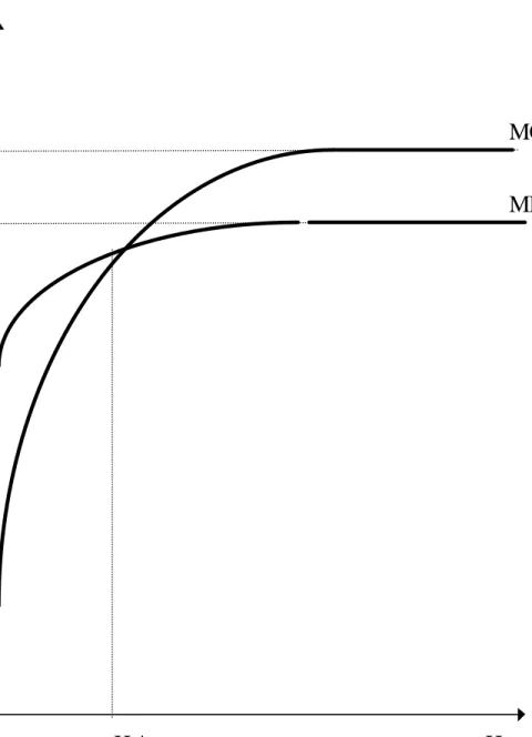
These choice equations tell us that the gains from re-allocation include the value of the labor that is freed up due to the re-allocation in addition to the net gain in income when the parcel is allocated between two contracts with different average products. The left hand and right hand sides of equations [26]-[28] can be interpreted as the marginal revenue and marginal cost of the re-allocation respectively. For the re-allocation from owner-farming to sharecropping [26], the first two terms of marginal benefit represent the average product of sharecropped land net of the opportunity cost of the tenant’s time evaluated at the market wage. The third terms depicts the value of landlord’s time freed due to the re-allocation evaluated at the marginal product of the landlord’s time. The marginal cost, on the other hand, is the average product under owner-farming. Figure 1 illustrates the marginal revenue and cost as a function of the proportion of sharecropped land (Hs/H). The slopes of these functions are:

marginal benefit (MR): − _Z w > H s s 1* ∂ 0 ∂ [30] marginal cost (MC): − Z w > H o s 1* ∂ 0 ∂ since ∂ ∂ w Hs < 0 .

The average products and the shadow wage are sensitive to the allocation of land across contracts. When the landlord allocates Hs units of land to sharecroppers, he or she must equate the marginal products of time allocated to owner-farming (Ho) and sharecropping (Hs). The labor allocation condition implies that when labor is freed up due to land re-allocation, most of it must be assigned to owner-farming. Therefore, as the slope equations [30] indicate, the marginal cost increases at the faster rate than the marginal revenue because most of the re-allocated time is assigned to owner-farming, and owner-farming thus gains relatively more from the increase in Hs. If MR=MC for some Hs, mixed-tenancy arises with some of the land share-cropped and the remainder, owner-farmed. The sufficient condition for the existence of sharecropping is,

MR>MC when Hs=0 [31]

and the sufficient condition for mixed tenancy is [31] and

MR<MC for large enough Hs [32]

Using equations [27] and [28], the choice between owner-farming and fixed-rent contracts and the choice between fixed-rents and share-rents can be analyzed in a similar way. An important difference is that an increase in fixed-rent farming has a positive external effect on both owner-farmed and sharecropped land. When the marginal unit of land is fixed-rented, both the time inputs Zo and Zs increase and the shadow wage (w) converges to the market wage, u. This results in a relatively steeper slope for the marginal cost function compared to the case illustrated in figure 1. However, the optimal time input in the fixed-rented land, zf is not affected by the re-allocation. By easing the landlord’s time constraint, fixed rent contracts

facilitate the replacement of inefficient (in the Marshallian sense) sharecropping with first-best owner-farming. A fixed rent contract will be chosen if the loss in average product due to skill deficiency is outweighed by the gains due to higher time inputs in owner-farming and sharecropping.

The existence of mixed-tenancy depends on condition [32]. When Hs increases, the marginal product of landlord’s time converges to the market wage, u. For large enough H, the landlord may be able to achieve the optimal levels of Zo*and Zs* for some Hs. In this case, the landlord’s time allocation per unit land and thus the average product under each arrangement is independent of land allocation choices (Hs and Hf). As a result, he can freely re-allocate land between owner-farming, sharecropping and fixed-lease renting without changing the time inputs Zo* and Zs*, and the optimal time input choices are separated by the exogenous market wage, u. The straight-line segments in the MR and MC functions in figure 1 depict this scenario. The condition [32] is then determined by the relative magnitudes of the following optimal average product functions:

(

)

(

)

(

)

f_o* = f_o Z_o*_{( , )}u S _, f_s* = f_s Z_s*_{( , , , )}u v α S _, f_f* = f_f z*_{f( , )}v s _[33]

Since the landlord’s time allocation is separable and all three average revenue functions are independent of land allocation choices Hs and Hf , equations [26]-[28] reduce to:

fs v z s u Zo Z s f * * * * * . ( ) − 2 + − 1 > 0 [34] f _f* − v z*_f + u Z_o* > f₀* [35]

f

−

vz

+

u Z

1

>

f

−

v z

.

2

The choice between owner-farming and sharecropping now depends only on the relative market wage and the output share. Specifically, owner farming is preferred to sharecropping if the opportunity cost of using the landlord’s time for unskilled labor is smaller than enforcement costs associated with sharecropping. Owner farming is preferred to fixed rent farming if the opportunity cost of using landlord’s time is smaller than the gains from using landlord’s farming skills. In addition, if skills are relatively more important to

production than time, as represented by a large x in [2], the incidence of owner-farming will be higher. Finally, Sharecropping is preferred to fixed-rent farming if the landlord’s skills are relatively high, Marshallian inefficiency losses are low, and the opportunity cost using landlord’s labor is small. Here again, the incidence of sharecropping increases when skills becomes relatively more important than time.

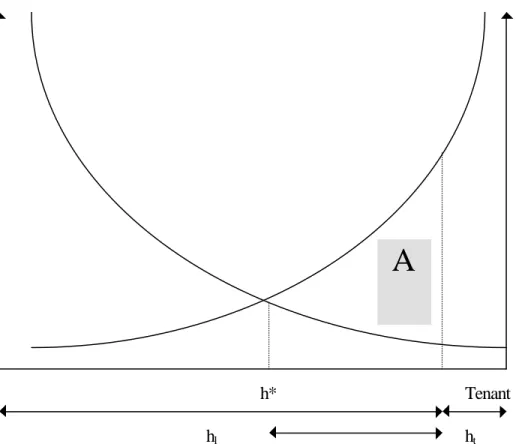
The basic result of the resource adjustment model is summarized in Figures 2 and 3. Figure 2 illustrates the case where the landlord owns more land (hl) than the tenant (ht) but has identical endowments of both time and skill. It is clear that a Pareto superior outcome can be achieved by re-allocating h*-ht units of land from the landlord to the tenant under a fixed-rent contract. Since the provider of both time and skill is assigned the entire residual under both owner-farming and fixed-rent farming, the marginal product functions are identical mirror images in figure 2. The shaded area (A) shows the gains from contracting. The gains are large when the two parties differ only in terms of their land endowment.

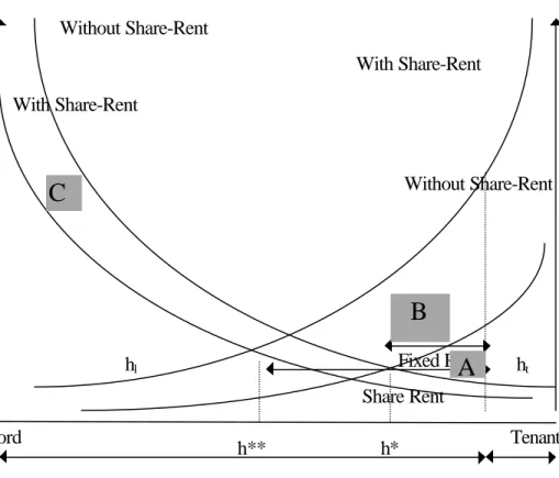
However, tenants are likely to have lower skill levels than landlords in most rural economies.16 If the tenants are relatively unskilled, as shown in figure 3, the gains from fixed-rent contracting (area A) are much smaller. In this case, sharecropping provides an alternative mechanism where the landlord and tenant specialize in the inputs they are better endowed with.

As shown in figure 3, the marginal product function for sharecropping is similar to that of owner-farming because the landlord compensates for the low skill level of the tenant. However, sharecropping introduces two new costs to the equation: first, the standard Marshallian inefficiency arises because the residual is shared by both parties, and second, the landlord must re-allocate some time away from his or her own farm to provide skilled inputs in the sharecropped land. Such a re-allocation of inputs away from the owner-farmed land when the landlord engages in sharecropping was observed in Indian state of

We do not claim that this is necessarily the case. For example, relatively more skilled tenants are observed in the case of absentee landlords who have no experience in farming and in the case of landlords who are impoverished due to the exceedingly small size of their inherited holding.

Punjab by Bell, Raha and Srinivasan [1995]. They call this a “dilution effect”. The decision to sharecrop lies primarily on the trade-off between the gains from specialization in the sharecropped land net of the enforcement costs (area B) and the loss of landlord’s time in the owner-farmed land (area C). The gains from sharecropping will be large if the differences in skills are large and the marginal

cost of re-allocating time is small. Sharecropping may arise when the tenants have relatively low skills, and the landlord is able to provide skilled inputs with minimal effects on his or her own farm (minimum dilution effects).

Comparative Statics: The Effect of Skills and Outside Options

As indicated earlier, the effects of relative management skills and the outside labor market options on contract choice are different for small and large farms.17 The owner-farming-sharecropping trade-off is independent of the relative skills of the landlord for small enough farms. In both cases, owner-farming is chosen when the outside option of the landlord is relatively low. Fixed-rent contracts are chosen when tenants are relatively skilled and the landlord’s outside options are relatively high. As the relative skill of the landlord increases, the outside option must rise correspondingly larger for a fixed-rent contract to arise. Absentee-landlords are an example of relatively unskilled landlords with high outside options. Sharecropping is preferred when the landlord’s outside options are high enough to make owner-farming (the provision of both M1 and M2) unprofitable, but relative management skills of the landlord are sufficiently high to make sharecropping preferable to fixed-rentals. Therefore sharecropping is observed when the landlords are skilled at farming but do not have enough time, given their outside options, to engage in self-cultivation.

The analysis of large farms is somewhat different. In the large farm, since the landlord’s labor

time constraint is binding, the landlord must allocate his or her time so that the income from the entire holding, not an individual parcel, is maximized. For example, he or she must choose between owner-farming a small parcel and fixed-leasing the remaining large portion of the holding, or specializing in share-cropping the entire holding. The first choice avoids enforcement costs but may involve skill costs if the fixed-rent tenants are inept at management, and vice versa. Therefore, for large farms, the choice is two-fold: 1) owner-farming a small portion of the holding and fixed-leasing the remaining large portion, and 2) share-cropping a large portion of the holding and fixed-leasing the remaining (if any) small portion. The first is preferred if the tenant is relatively skilled (so fixed-leasing is not inefficient), and the second choice is preferred if the tenant is relatively unskilled. The trade-off between share-rents and fixed-rents is represented by net gains from the skills used, the re-allocation of landlord’s time, and the enforcement costs in sharecropping. The greater the time constraint, and higher the marginal value of landlord’s time, fixed-rent contracts are preferred.

If the landlord’s outside option increases, the incidence of fixed-rent contracts increase. On the other hand, increasing outside options of the landlord makes sharecropping more attractive than owner-farming. Therefore, an increase in landlord’s outside options has a positive effect on both fixed-rent contracts and share-cropping at the expense of owner-farming. Unlike in the small farm case, no single contract is necessarily optimal for the entire holding. The optimal solution, for large enough farms, may be a combination of all three types of contracts.

3. The Empirical Specification

The underlying framework of our analysis is the simple leasing model of Bliss and Stern [1982]. Suppose that farmer i owns Fi units of family labor, Xi units of bullocks, and Hi units of land. Then, if the markets for labor, and bullocks are imperfect, the desired cultivated area (Ci) is

where Zi is a vector of all other characteristics of the farmer. Then, the notional demand for land (Y*i) in

the land leasing market is;

Y

C

H

f F X Z

H

*

( ,

,

)

=

−

=

−

The difference between the actual and notional demands for land depends on the transaction costs in the land leasing market. Suppose the actual net amount of land leased-in is Yi. Then

Y

=

h Y

(

)

=

h f F X Z

( ( ,

,

)

−

H

)

The Choice of Contract

The main hypothesis of this paper is that relatively skilled tenants obtain fixed-rent contracts while those endowed with family labor get share contracts. The theoretical analysis showed that the level of managerial skill required to enter in to a sharecropping contract is less than that for a fixed-rent contract because the landlord typically provides some of the skill-intensive managerial inputs in sharecropped farms. The empirical model presented in this section identifies some key differences between the two contracts as resource adjustment mechanisms.

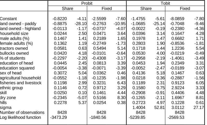
We focus on the leasing behavior of tenants because data constraints prevent us from estimating a more general model that includes the landlords. The simplest method of estimating the determinants of sharecropping and fixed rent leasing is to carry out separate leasing or contract choice estimates for each type of contract. The starting point of our analysis is probit and tobit models for the following underlying equations based on the model outlined in [37]-[39]:

S

F

H

X

Z

F

F

H

X

Z

=

+

+

+

+

+

=

+

+

+

+

+

β

β

β

β

β

ε

δ

δ

δ

δ

δ

ϕ

where εi and ϕi are distributed N (0, σε2) and N (0, σϕ2) and Si* and Fi* are the underlying variable for sharecropping and fixed-rent leasing, Fi, is the endowment of family labor, Hi is the amount of

land owned, Xi are the other owned farm inputs, and Zi is a vector of farmer characteristics that includes skill.

A well-documented flaw of the single equation tobit model is its inability to distinguish the two distinct, albeit related, events of leasing-in and choice of contract. For example, we expect farmers who own little land to lease-in relatively more land under either contract. However, among the tenants, those with more assets, including land, may prefer fixed-rent contracts. A multi-stage generalization of this model is needed to separate the three different stages of the decision making process; 1) the choice to lease-in, 2) the choice of contract, and 3) the extent of land leased-in.

Two alternative methods are used to model the first two stages. In the first method, a multinomial logit model is used to combine the first two choices in to a single decision between three alternatives. In the second method, the two stages are modeled as sequential probit equations with the contract choice observed only when the choice to lease-in is made. The extent of land leased-in is modeled in the next section as a linear regression for each type of tenant with appropriate corrections for sample selection computed from the choice equations.

Multinomial Logit Model of Contract Choice

A standard multinomial logit specification is used with the choice variable Y where: Y = 0 if land is not leased-in

1 if land is leased-in under a share-contract 2 if land is leased-in under a fixed-rent contract and

Prob

(

)

for

, ,

and

' '

Y

j

e

e

j

=

=

+

=

=

∑

β

1

0 1 2

0

The coefficients estimates, βj, can then be interpreted as the marginal effect of xi on the relative log odds ratio between the choice j and choice 0.

Bivariate Probit Model of Contract Choice

The bivariate probit model jointly estimates probit equations for the leasing and contract choices with correlated error terms. The specification of this standard model is

L

x

L

L

S

x

S

N

,

,

,

,

,

~

( , ,

,

, )

=

+

=

>

=

+

=

>

β

ε

β

ε

ε ε

σ σ ρ

1

0 0

1

0 0

0 0

if

otherwise

S

if

otherwise

where L* and S* are the underlying choice variables for the extent of land leased-in and the extent of land sharecropped, L and S are the observed choices and x is a vector of explanatory variables that includes F, X, H and Z. The functional form is used to identify the model with the same set of explanatory variables in both equations because it is difficult to find identifying variables for either equation.

Since we do not observe the contract choice for the farmers who choose to self-cultivate, the standard model must be modified to incorporate the fact that the contract choice (S) exists only if the leasing choice (L) is positive. This gives rise to a bivariate probit model with three types of probabilities:

Prob( = (- Prob( = ( Prob( = 0) = (1) - ( (2) 1 - ( ' L S x x L S x x L x x = = − = = 1 0 1 1 2 2 2 1 1 2 2 2 1 1 1 1 1 1 , ) , , ) , ) , , ) ), ) ' ' ' ' ' Φ Φ Φ Φ β β ρ β β ρ β β [43]

The first specification, proposed by Wynand and van Praag (1981), treats S as a truncated variable at L=0. The second variant, due to Meng and Schmidt (1985), defines S as a zero-censored variable when L=0. The obvious difference is that the latter method treats the choice to reject leasing-in

as an indicator of a simultaneous decision to reject sharecropping. As a result, owner-farming and fixed-rent farming are pooled as a common alternative to sharecropping.

The Land Extent Equations

We also carry out least squares regressions for the extent of land leased by each type of tenant to determine whether this adjustment process occurs within each group. If the evidence of adjustment is weak within groups, we can conclude that the adjustment process is carried out primarily in the first stage where contracts are assigned to the tenants, and not by the size of the farm allocated to each tenant. This result would confirm the claim of the theoretical model that type of contract, and not the individual farm size, is the key choice variable in the leasing model. Since tenants of either type are a subset of our sample, selectivity correction terms are included to obtain consistent estimates. We follow a two-step method analogous to that of Heckman [1976] where the predicted probability of the subset is estimated in the first stage, and a selectivity correction term based on this predicted probability is included in the second stage linear regression to obtain consistent estimates of the parameters. The only difference from Heckman’s original method is the use of multinomial and bivariate probit equations for selection. The leasing equation for observations with Y=j is,

H

=

β

'

x

+

θ λ

+

η

The selectivity terms, λj, are constructed from the predicted probability of choice j computed from the choice equations. If the multinomial logit model is used as the selection equation, the selectivity term, λj, is calculated using the predicted probability for Y=j (equation [41]).

λj φ j j j j H H H P = ( ) = − ( ), ( ) Φ where Φ 1 [45]

and φ and Φ are the standard normal PDF and CDF18. If the bivariate probit model is used for selection, the selectivity term is calculated in the same way using the appropriate predicted probability from [43].

The Index of Farming Skills

The biggest obstacle to understanding the role of management or entrepreneurial skills in land leasing is the absence of an appropriate measure of skill. Management skill or capacity has several dimensions including “(1) drives and motivations, e.g. farmer’s goals and risk attitude; (2) abilities and capabilities, e.g. cognitive and intellectual skills; and (3) biography, e.g. background and experience” [Rougoor et. al. 1998]. While some aspects of skill such as education and age are easily measured, many others such as drive, motivation, entrepreneurship and ability are neither directly observable nor quantifiable.

Farm studies have used two distinct approaches to measure management skills. The first, based on Mundlak [1961], treats management inputs as the time invariant portion of the production function residual. Skoufias [1991] uses this method to estimate a linear land leasing equation using panel data from India. However, the panel data fixed effects estimation is clearly unsuitable in our context because many explanatory variables such as asset ownership have negligible time (within) variation compared to the cross-sectional (between) variation.19 More fundamentally, by focusing solely on the residual, the panel data methods fail to make use of the observed dimensions of skill such as education and experience.

The second approach is the inclusion of observed variables that are assumed highly correlated with managerial skill. Bliss and Stern, Nabi and Skoufias [1991] include age, education and caste as

This model is proposed in Lee [1983]. This paper also describes the corrected asymptotic covariance matrix for the two-step estimator.

19

Skoufias himself points out, for example, his land ownership coefficient is biased as a result.A solution to the fixed effects problem is proposed by Lanjouw [1999] who models the error structure explicitly with in a joint maximum likelihood estimation of leasing and production functions.

proxies. Pant [1983] includes the value of farm implements. However, these proxy variables may have an independent effect on land tenancy that cannot be separated out by including them directly in an OLS regression. For example, education may have a positive effect on leasing by improving access to market information or a negative effect by improving non-farm outside options, two effects that are quite independent of the positive skill effect. Therefore, there is no a priori basis to identify any of the farmer characteristics as indicators of skill.

In this paper, we combine these two approaches by interpreting farming skill as the contribution of a farmer’s observed characteristics to the farm’s productive efficiency. Farming skills are defined as a weighted average of the tenant’s observed characteristics (such as age, education, household demographics, types of non-farm activity and wealth). Since there is no a priori basis to assign values to the weights, they are computed by estimating the predicted contribution of farmer characteristics to farm efficiency. The simplest method is to include a vector of farmer characteristics directly in a production function. We use a conceptually similar method, but give a more appropriate structure to the estimates by using a stochastic production frontier method.

The stochastic production frontier, first proposed by Aigner et. al [1977] and Meeusen and van der Broeck [1977] is a production function with two error terms, a random disturbance term, εi, that is independent and identically distributed, and a one-sided non-negative error term, ui, that is distributed independently of εi. 20 The former captures both the effects of unobserved stochastic factors (e.g.weather shocks) and errors due to mis-specification of the model, and the latter represents “technical inefficiency” of the farmer or, more precisely, the ratio of the observed to maximum feasible output, where maximum feasible output is determined by the stochastic production frontier [Lovell 1993]. This structural model is more appropriate for our purposes because it explicitly recognizes the non-linearity of

the production function and separates the technical efficiency (one-sided) component of the residual from other unobserved stochastic (two-sided) effects.

The production frontier, where Q is the output, and Z is a vector of observed inputs, such as land, labor, fertilizer, seeds, machinery and draft animals is defined as follows:

Q

f Z

u

where u

U

and U

N

and

N

=

−

=

(

; ) exp(

)

~

( ,

)

~

( ,

)

β

ε

σ

ε

σ

0

0

We assume that the two error terms are distributed normal and half-normal respectively. If ui =0, production is at the stochastic frontier. Then, from [46], the technical efficiency (TEi) of farmer i is,

TE Q f Z u i i i i = = − [ ( ; ) exp( )]β ε exp ( ) [47]

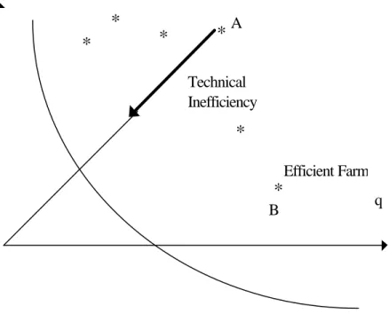
The concept of technical efficiency can be illustrated using a simple isoquant diagram with land and labor as the two inputs [figure 4]. The isoquant q defines the frontier, or the set of efficient choices of inputs for a given output level. Points such as A and B represent actual observed input choices for the output level q. Assuming that the observed land-labor ratio is efficient, i.e. there is no allocative inefficiency, technical efficiency of the farm is given by the distance between the observed point and the frontier along the ray that represents the actual input ratio. Point B represents a technically efficient farm because the distance to the frontier is zero.

This estimate of technical efficiency (TE) is independent of stochastic errors and measures the degree to which a farmer comes close to achieving the best possible outcome conditional on his or her input choices and the production technology.21 Technical efficiency in farms may be determined by the

Although it is straightforward to estimate the stochastic frontier model using maximum likelihood methods, the derivation of a technical efficiency measure (TEi) for each farmer is difficult because the two components of the error term cannot be easily decomposed. We use the functional form proposed by Jondrow et. al [1982] and generally accepted in the literature for the conditional distribution of the one-sided error term to express the conditional mean of the one-sided error term:

characteristics of the farmer, the land, the climate and, in the case of share-tenancy, the landlord.22 For example, landlords may compensate for the low skills of the less able tenants by providing some or all of the skilled inputs in a sharecropping arrangement. Therefore, two farms can have the same technical efficiency even though the tenants’ skill levels are quite different. An accurate measure of farming skills must isolate the farmer’s contribution to technical efficiency. The one-sided error term, u, can be expressed as follows:

u

= −

log

TE

=

a F

+

(

a d

+

a d

)

L

+

a H

+

e

where F is a vector of farmer characteristics, L is a vector of landlord’s characteristics and H is a vector of geo-climatic variables that include soil quality, gradients, irrigation, rainfall, humidity and temperature. ds and df are dummy variables for share and fixed-rent tenancy and ei is a random i.i.d. error term which is uncorrelated with the included variables.

Farmer skills can be defined as the farmer’s contribution to technical efficiency, or a1Fi in equation [48]. In order to fully capture the many dimensions of skill, the vector Fi includes not only variables such as education and age, but other farmer characteristics that are likely to be correlated with unobserved aspects of skill such as motivation and ambition. Ownership of non-farm assets and types of non-farm activity are included as potential indicators of such attributes. Since the weights of each factor are econometrically derived, the best approach is to include as large a set of farmer characteristics as possible in the efficiency equation. A consistent estimate of skill can be obtained only if the parameter a1 is consistently estimated. Unfortunately, since our data set does not match tenants with landlords, landlord’s characteristics cannot be included in equation [48]. Because tenants and landlords are matched in a systematic non-random manner, the estimate of a1 will thus be biased. We avoid this problem by estimating the frontier only for the self-cultivators to obtain the coefficient estimates and then using these

Some studies have interpreted the technical efficiency term as a measure of skills. Kirkley et al. [1998], for example, argue that differences in technical efficiency account for differences in skills between fishing boat captains who use

estimates to compute predicted values for the entire sample. Therefore, definition of farming skills is modified to mean the contribution of farmer attributes to technical efficiency if the farmer were a self-cultivator.

We include district-level dummy variables to account for broad regional agro-climatic characteristics. Since only irrigation variables are available as farm level measures of land quality, farm-level variation in land quality that is not correlated with irrigation may be left out. It can be argued that some of this residual land quality reflects high skill levels of the farmer, such as the skillful management of soil quality, and legitimately belong in the predicted skill index. If the remaining unobserved land quality is correlated with observed farmer characteristics, the predicted skill estimates are biased. The implications of this problem are discussed in detail in under specification problems.

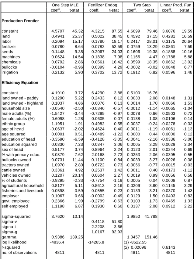
The last stage in constructing the skill index requires the estimation of equation [48] for the self-cultivators. Prediction efficiency equations are commonly estimated by regressing the technical efficiency estimates obtained from the stochastic frontier estimation on a set of explanatory variables [Pitt and Lee 1981, Kalirajan 1981, Kirkley et al 1998]. Several recent studies [Kumbhakar et. al 1991, Reifschneider and Stevenson 1991, Huang and Liu 1994, Battese and Coelli 1995] have pointed out that such a two-step method is fundamentally incorrect because the dependent variable in the second step is assumed one-sided, non-positive and identically distributed in the first step. A more appropriate method is to estimate the parameters of equation [48] jointly with those of the stochastic frontier using maximum likelihood methods using consistent distributional assumptions on the error structure. We use the version of this method proposed in Battese and Coelli [1995].

The frontier-based skill index has its share of problems that include 1) strong distributional assumptions on the error structure, 2) inconsistency of the technical efficiency estimator, and 3) endogeneity problems. The distributional assumptions are common to most maximum likelihood methods.

However, it is possible to use a variety of distributions, such as half-normal, truncated normal and exponential to model the one-sided error term [Greene 1993b].23 In addition, the estimates from the frontier model can be compared to linear production function estimates to test whether our index is particularly sensitive to the distributional assumptions. The inconsistency of the efficiency estimator is more difficult to circumvent in cross-sectional models.24 Fortunately, the estimator is unbiased and the inconsistency is caused by the fact that the variance is independent of the sample size. The endogeneity issues are dealt with in detail in the following two subsections.

Specification Issues I: Endogenous Inputs in the Production Frontier

The direct estimation of production functions has been criticized because inputs are typically jointly determined with the output [Mundlak 1961]. In the production frontier, the parameters as well as technical efficiency may be inconsistently estimated if technically efficiency is correlated with inputs [Kumbhakar 1987, Kalirajan 1990, Kumbhakar et. al 1991].

The literature has responded to this issue in two ways. Many studies have invoked the well-known arguments of Zellner et. al [1966] to assume that input choices are exogenous in an stochastic agricultural production environment.25 However, as Kumbhakar [1987] points out, this assumption holds only if technical efficiency is unknown to the farmer. A solution to the endogeneity problem is the joint estimation of the frontier and its first order conditions in a profit maximizing framework [Kumbhakar 1987,

23

Semi-parametric methods that are independent of functional assumptions have not yet been developed. 24

Battese and Coelli [1988] develops a consistent estimator for panel data. 25

Two recent examples are Battese and Coelli [1995] and Kirkley et. al. [1998]. Greene [1993] surveys some of the earlier papers.

Kalirajan 1990, Kumbhakar et. al 1991] 26. This specification has sound micro-economic foundations, and treats both inputs and outputs as endogenous variables. The profit maximization method is obtained by adding allocation equations for each endogenous input j to the stochastic frontier defined in equation [48]. For inputs such as fertilizer and pesticides that are obtained in competitive markets with exogenous prices, the allocation equations are just the first order conditions of profit maximization:

w

=

p MP

.

exp(

v

)

where j indexes inputs, wj is the exogenous input price, p is the output price, and MPj is the marginal product of input j. The random variable vj is a two-sided error term that measures allocative inefficiency, or the degree to which the farmer fails to satisfy the first order condition. This error term can be interpreted as noise in the price signal that may be a result of imperfect information or measurement error, or as errors in optimization. It is also assumed that input and output prices are exogenously given, and that the technical efficiency is known to the farmer. The technical efficiency term enters the first order condition through the marginal product (MPj) term.

This method can be used only if reliable price data are available and is limited to inputs that are traded in a competitive market (with exogenous prices). In this paper, we estimate the frontier with fertilizer as an endogenous input. The lack of suitable price data prevents us from estimating a complete set of first order conditions. First order condition of this type cannot be formulated for inputs such as land, animals and even labor, which are not traded in competitive markets at exogenously determined prices. As a result, we assume the exogeneity of these inputs.

Several other studies have used a cost minimization framework where input levels are treated as endogenously determined for given prices and technologies [Schmidt and Lovell 1979, Greene 1980, Kumbhakar 1997]. While the behavioral assumption of cost minimization has a clear economic interpretation, the assumption of an exogenous output level is clearly inappropriate except in the case of certain regulated environments. In addition, since price data show very little variation (compared to input levels) in most household-level surveys, cost functions are difficult to estimate. Finally, technical complications arise in the definition of allocative efficiency as a one-sided error in the cost function and a two-sided term in the share equations[Bauer 1990]

Fortunately, the potential endogeneity of land in the production function does not affect the power of our tests in the leasing model because the skill variable is unbiased by definition under the null hypothesis that farming skills do not affect land leasing decisions. It must be emphasized however that, if the null hypothesis is rejected, the coefficient of the skill variable in the leasing equation cannot be reliably interpreted as the magnitude of the effect of skill on leasing since the land input is in fact correlated with skills.

Specification Issues II: Endogeneity in the Leasing Equation

Another potential problem in our specification is the possible correlation of farming skills and the error term in the leasing equation. The stochastic two-sided error term removes some of these effects, such as weather shocks, from the technical efficiency estimates. More factors are removed in the second stage when the predicted values are obtained. But some unobserved factors that affect the leasing choice may remain in the skill index if they are correlated with observed farmer characteristics. If, for instance, the skill index includes some elements of unobserved land quality, the coefficient on technical efficiency in the leasing model will be biased. We include irrigation and district dummy variables to control for some of the land quality differences. Any remaining unobserved land quality effects may be picked up by the skill variables and reduce the power of our tests.

We resort to theoretical arguments to assert that potential endogeneity problems in the skill variable do not affect our conclusions on contract choice. The null hypothesis that skills do not affect the choice of contract will be incorrectly rejected if the effect of both skill and unobserved land quality have the same sign. Fortunately, the theoretical literature on the relation between land quality and contract choice comes to a different conclusion, that sharecropping is used as a mechanism to minimize “land mining” or “land quality abuse” by tenants [Murrell 1983, Datta et al 1986, Ray 1998, DeWeaver and Roumasset 1999]. In these land mining models, fixed-rent contracts are offered only under conditions

where the scope for land mining is limited. Examples of such condition