Measurement Errors of Expected Returns Proxies and the Implied
Cost of Capital
(Article begins on next page)
The Harvard community has made this article openly available.
Please share how this access benefits you. Your story matters.
Citation
Wang, Charles C.Y. "Measurement Errors of Expected Returns
Proxies and the Implied Cost of Capital." Harvard Business School
Working Paper, No. 13–098, May 2013.
Accessed
February 19, 2015 12:02:58 PM EST
Citable Link
http://nrs.harvard.edu/urn-3:HUL.InstRepos:10647827
Terms of Use
This article was downloaded from Harvard University's DASH
repository, and is made available under the terms and conditions
applicable to Open Access Policy Articles, as set forth at
http://nrs.harvard.edu/urn-3:HUL.InstRepos:dash.current.terms-of-use#OAP
Copyright © 2013 by Charles C.Y. Wang
Working papers are in draft form. This working paper is distributed for purposes of comment and discussion only. It may not be reproduced without permission of the copyright holder. Copies of working papers are available from the author.
Measurement Errors of
Expected Returns Proxies and
the Implied Cost of Capital
Charles C.Y. Wang
Working Paper
13-098
Measurement Errors of Expected Returns Proxies
and the Implied Cost of Capital
Charles C.Y. Wang
∗ Harvard Business SchoolMay 2013
Abstract
This paper presents a methodology to study implied cost of capital’s (ICC) measure-ment errors, which are relatively unstudied empirically despite ICCs’ popularity as proxies of expected returns. By applying it to the popular implementation of ICCs of Gebhardt, Lee, and Swaminathan (2001) (GLS), I show that the methodology is useful for explaining the variation in GLS measurement errors. I document the first direct empirical evidence that ICC measurement errors can be persistent, can be associated with firms’ risk or growth characteristics, and thus confound regres-sion inferences on expected returns. I also show that GLS measurement errors and the spurious correlations they produce are driven not only by analysts’ systematic forecast errors but also by functional form assumptions. This finding suggests that correcting for the former alone is unlikely to fully resolve these measurement-error issues. To make robust inferences on expected returns, ICC regressions should be complemented by realized-returns regressions.
Keywords: Expected returns, implied cost of capital, measurement errors.
JEL: D03, G30, O15, P34
∗[email protected]. I am grateful to Nick Bloom, Han Hong, Dave Larcker, and Charles Lee for their advice and support on this project. I also thank Travis Johnson, Paul Ma, Jim Naughton, Maria Ogneva, Eric So, Luke Stein, Johannes Stroebel, Xu Tan, Gui Woolston, participants of the Stanford applied economics seminar, the Stanford Joint Accounting and Finance seminar, and seminar participants in Columbia GSB, Harvard Business School, and Stanford GSB for their helpful comments and suggestions.
1
Introduction
The implied cost of equity capital (ICC), defined as the internal rate of return that equates the current stock price to discounted expected future dividends, is an increasingly popular class of proxies for the expected rate of equity returns in accounting and finance.1 Three primary factors have contributed to the rise in ICCs’ popularity over the past fifteen years. First, ICCs have intuitive appeal, in that they are anchored on the discounted-cash-flow valuation model. Second, unlike realized returns or the traditional factor-based models, ICCs are forward-looking and utilize forecasts of a firm’s future fundamentals (e.g., consensus analyst forecasts of future earnings). Third, ex-post realized returns and the traditional factor-based models are often considered too noisy.2
This intuitive appeal has given rise to a body of literature that uses ICCs to study the cross-sectional variations in expected returns, whereby researchers run regressions of ICCs on various firm characteristics or regulatory events to make inferences on expected returns.3 However, the unknown properties of ICC measurement errors—the difference
between the ICC and the (unobserved) true expected returns—represents a challenge to the use of ICCs and the inferences from regression results. When interpreting regressions of ICCs on firm characteristics, the researcher is uncertain of whether the regression coefficients capture the systematic associations of firm characteristics with expected re-turn or with ICC measurement errors. Adjudicating between these possibilities requires
1That is, ICCs are the
b
eri,t that solves
Pi,t= ∞ X n=1 Et[Di,t+n] (1 +erbi,t) n,
wherePi,t is firmi’s price at timet, andEt[Di,t+n] is the timet expectation of the firm’s dividends in periodt+n.
2Fama and French (1997) noted that these factor-based estimates are “unavoidably imprecise” and that empirical problems “probably invalidate their use in applications.” Consistent with this assessment, the recent evidence of Lee, So, and Wang(2012) documents that these factor-based estimates perform poorly relative to other classes of ex ante measures of expected returns, such as ICCs, in terms of cross-sectional and time-series measurement-error variance.
3For example,Botosan(1997) studies the impact of corporate disclosure requirements;Chen, Chen,
and Wei(2009) andChen, Chen, Lobo, and Wang(2011) examine the impact of different dimensions of corporate governance;Daske(2006) examines the effect of adopting IFRS or US GAAP;Dhaliwal, Krull, Li, and Moser (2005) examines the effects of dividend taxes; Francis, LaFond, Olsson, and Schipper
(2004) study the effects of earnings attributes;Francis, Khurana, and Pereira(2005) study the effects of firms’ incentives for voluntary disclosure; Hail and Leuz (2006) examine the effect of legal institutions and regulatory regimes; andHribar and Jenkins(2004) examine the effect of accounting restatements.
an understanding of the properties of ICC measurement errors. For example, if ICC measurement errors are classical—independently and identically distributed with zero mean—then in large sample the estimated regression coefficients reflect associations of firm characterisitcs with expected returns. On the other hand, to the extent that ICC measurement errors are systematically correlated with firm characteristics, researchers’ inferences may be confounded by spurious correlations with measurement errors.
Ex ante, I expect two primary sources of ICC measurement errors, each of which has the potential to be systematically associated with firm characteristics and thus to confound regression inferences. The first source of ICC measurement errors is forecast errors of future fundamentals (e.g., cashflows or earnings). To the extent that such forecasts are systematically biased toward certain types of firms, the resulting ICCs can be expected to contain measurement errors that are correlated with the characteristics of such firms. For example, La Porta (1996);Dechow and Sloan (1997); Frankel and Lee
(1998); andGuay, Kothari, and Shu (2011) show that consensus analyst EPS (as well as long-term growth) forecasts tend to be more optimistic for growth firms. Thus, all else equal, ICCs constructed using these analyst forecasts could produce measurement errors that are systematically more positive for growth firms than for value firms.
A second source of ICC measurement errors is model misspecification, which results from erroneous assumptions embodied in the functional form that maps information and prices to expected returns. If the extent of model misspecificaton varies with firm type, ICC measurement errors can be expected to be correlated with firm characteristics even if forecasts of future earnings are unbiased. For example, Hughes, Liu, and Liu (2009) show that when expected returns are stochastic but ICCs implicitly assume constant expected returns, ICCs differ from expected returns and ICC measurement errors can be correlated with firms’ risk and growth profiles, even if forecasts of future cash flows are perfectly rational. As a consequence, despite a concerted effort to understand and mitigate the impact of systematic forecast biases on ICC measurement errors (e.g.,Easton and Sommers, 2007;Hou, Van Dijk, and Zhang, 2012;Guay et al.,2011; Mohanram and Gode,2012), it is still possible for ICCs to produce measurement errors—resulting from
model misspecification—that are systematically correlated with firm characteristics and confound inferences.
Because the empirical properties of ICC measurement errors are relatively unknown, and because their effects and implications are critical to empirical research that seeks to understand cross-sectional variation in expected returns, Easton (2009) concluded in his survey of ICC methodologies that “as long as measurement error remains the
Achilles’ Heel in estimating the expected rate of returns, it should be one of the focuses of future research on these estimates.” (p.78) Echoing such sentiments, Lambert (2009) commented that “[there are likely] biases and spurious correlations in estimates of implied cost of capital. The next step should be to try to develop procedures to try to correct for these problems.” The goal of this paper is to shed light on the cross-sectional properties of ICC measurement errors and to document their drivers that could lead to spurious inferences in regressions.
The paper presents, for a type of expected return proxies, a procedure for estimating the cross-sectional associations between their measurement errors and firm characteristics; such an associations are important in understanding the properties of regression depen-dent variables. By applying this procedure to one of the most popular implementations of ICCs, colloquially known as GLS in recognition of its authors (Gebhardt et al.,2001), I show that the methodology is useful to explain GLS measurement errors. I also document four findings that contribute to the ICC literature. First, I present the first evidence that ICC measurement errors can be persistent, with an median annual AR(1) parameter of 0.48 for GLS measurement errors. Second, I document that GLS measurement errors are systematically cross-sectionally associated with firm risk and growth characteristics, such as market capitalization, book-to-market ratio, 3-month momentum, analyst coverage, and analyst long-term growth forecasts, characteristics that are commonly thought to explain the cross-sectional variation in expected returns. Third, I show that GLS mea-surement errors are driven not only by errors arising from analyst forecast biases but also by errors arising from the assumption of constant expected returns implicit in ICCs. Finally, I show that these measurement errors lead to spurious inferences in regression
settings, and that they can explain some puzzling associations previously documented in the literature, such as the negative association between GLS and stock price momentum. The empirical evidence presented in this paper has important implications for em-pirical research using ICCs. First, emem-pirical results involving cross-sectional regressions of ICCs on firm characteristics are likely confounded by spurious correlations between ICC measurement errors and firm characteristics. Thus, research questions about the effects of certain firm characteristics or economic environments on firms’ expected rate of returns cannot be answered satisfactorily without understanding or correcting for the po-tential spurious effects of measurement errors. Second, methodologies for mitigating ICC measurement errors such as portfolio grouping and instrumental variables are limited in effectiveness since common grouping variables or instruments (e.g., market capitalization and book-to-market ratio) are likely correlated with the measurement errors, as is the case of GLS. Third, correcting for systematic analyst forecast errors alone is inadequate in fully addressing ICC measurement errors, since the latter are also driven by errors arising from model misspecification (e.g., the implicit assumption of constant expected returns). As a result, I argue for the necessity of complementing any ICC regressions with regressions using realized returns to establish a robust association between expected returns and firm characteristics.
Section 2 of the paper describes the theoretical model and lays out the estimation procedures. Section3presents the empirical results. Section 4discusses the implications of the paper’s findings, and offers some practical recommendations for researchers.
2
Theoretical Model and Empirical Methodology
2.1
Motivation
To identify the relevant firm characteristics (zi,t) that explain cross-sectional variation in the (unobserved) expected rate of equity returns over the next period,
researchers typically examine the empirical association between some proxy of expected returns (erbi,t+1) and firm characteristics, where
b
eri,t =eri,t+wi,t (2)
andwi,t is the proxy’s measurement error. The standard approach assumes that expected returns are linear in firm characteristics (3) with standard OLS assumptions on residuals. Assume too that measurement errors of expected return proxies are linear in certain firm characteristics with standard assumptions on residuals (4).
eri,t = δ0+δTzi,t+εeri,t (3)
wi,t = β0+βTxi,t+εwi,t (4)
where (εwi,t, εeri,t)˜iid(0,0) ;
(εwi,t, εeri,t) and (zi,t,xi,t) uncorrelated
Because expected returns are not observable, researchers’ use of proxies implies that they will not be able to directly estimate the coefficients of interest, δT. Thus it is easy to see that associations between measurement errors and firm characteristics may produce biases and spurious inferences about δT.
Without loss of generality, suppose for illustration that zi,t = xi,t = Sizei,t, where
Sizei,tis firmi’s log of market capitalization at the beginning of periodt. Then, equations (2), (3), and (4) imply the following relation between the expected-returns proxy andSize.
b
eri,t = (δ0+β0) + (δ+β)Sizei,t+ εeri,t+εwi,t
If measurement errors are associated with Size (i.e., β 6= 0) then a regression of the expected-returns proxy on Size produces a biased estimate of δ, a bias resulting from the spurious correlation betweenSize and the measurement error (β) that confounds the researcher’s inferences on expected returns.
2.2
Model
As the preceding example illustrates, making inferences about unobserved expected returns requires an understanding of the measurement errors in the proxies used. This section develops a methodology to estimate the systematic cross-sectional association between ICC measurement errors and firm characteristics in regression settings under the linearity assumptions of (3) and (4). To do so, I impose structure on the time-series behavior of expected returns and measurement errors, structure that allows me to separate these two components of a proxy. In particular, I model both expected returns and the proxy measurement errors to follow AR(1) processes, with persistence parameters of φi and ψi and with (potentially) correlated innovations ui,t+1 and vi,t+1, respectively:
eri,t+1 = µui+φieri,t +ui,t+1; (5)
wi,t+1 = µvi+ψiwi,t+vi,t+1; (6)
where (ui,t, vi,t)0 ∼ iid (0,0)
0 , Σuv ,Σuv invertible; (7) |φi|,|ψi| ∈ (0,1) ; and (8) φi 6= ψi. (9)
The AR(1) assumption on expected returns (5) captures the idea that expected re-turns are persistent and time-varying.4 This assumption is common in modeling interest
rates (e.g., Cochrane, 2001; Duffie and Lando, 2001) and in modeling expected returns of equities (e.g., Conrad and Kaul, 1988; Poterba and Summers, 1988; Campbell, 1991;
P´astor, Sinha, and Swaminathan, 2008; Binsbergen and Koijen, 2010; P´astor and Stam-baugh, 2012;Lyle and Wang, 2013), and is broadly consistent with the observation that returns are predictable. By contrast, the AR(1) assumption about measurement errors is a new assumption in the literature meant to capture the possibility that measurement errors could be persistent and time-varying. This assumption has great intuitive appeal, 4As noted inCampbell(1990) andCampbell(1991), the AR(1) assumption on expected returns need not restrict the size of the market’s information set, and in particular does not assume that the market’s information set contains only past realized returns. The AR(1) assumption merely restricts the way in which consecutive periods’ forecasts relate to each other, and it is quite possible that each period’s forecast is made using a large set of variables.
particularly for studying the measurement errors of ICCs that rely on analyst forecasts of future fundamentals. Because analysts can be slow to incorporate new information (e.g.,
Lys and Sohn, 1990;Elliot, Philbrick, and Wiedman, 1995; Guay et al., 2011; So, 2013), for example due to an anchoring-and-adjustment heuristic, their forecasts and the result-ing ICCs may tend to exhibit persistent (but time-varyresult-ing) errors. Another possibility is that persistent model misspecification errors gives rise to persistent and time-varying measurement errors.
Note that both AR(1) parameters are assumed to be constant across time for a firm in the set up; moreover, while the persistence parameter of expected returns (φi) is firm-specific, the persistence of expected-returns-proxy measurement errors (ψi) is implicitly firm- and model-specific (i.e., dependent on the model that generates the proxy). Finally, I make the regularity assumption that the two processes are stationary (8), and the identifying assumption that, for each firm, the AR(1) parameters are not equal to each other (9). The necessity of the last assumption will become clear in the next section.
2.3
Empirical Methodology
The above setup yields a proxy for ICC measurement errors with desirable properties. Substitution of (5) and (6) into (2) and some simple algebraic manipulations produce
b wi,t:5 b eri,t+1−φierbi,t ψi−φi | {z } b wi,t(ψi,φi) = µui+µvi ψi−φi | {z } αi +wi,t+ ui,t+1+vi,t+1 ψi−φi (10) = β0+βTxi,t+αi+ εi,t+ ui,t+1+vi,t+1 ψi−φi (11) by the linearity assumption of (4).
5To show the algebraic steps:
b
eri,t+1 = eri,t+1+wi,t+1 by definition of expected-returns proxy
= (µui+φieri,t+ui,t+1) + (µvi+ψiwi,t+vi,t+1) by AR(1) assumptions = (µui+µvi) +φieri,t+ψiwi,t+ (ui,t+1+vi,t+1)
= (µui+µvi) +φierbi,t+ (ψi−φi)wi,t+ (ui,t+1+vi,t+1)
Thuserbi,t+1−φierbi,t = (µui+µvi) + (ψi−φi)wi,t+ (ui,t+1+vi,t+1)
Assuming for the present that the AR(1) parameters are observed by the researcher, b
wi,t(ψi, φi) is an empirically observable proxy for ICC measurement errors and, by equa-tion (10), contains three components: (1) a firm-specific constant (αi); (2) the unobserved measurement error (wi,t); and (3) iid mean 0 AR(1) innovations.
Under the linearity assumption relating ICC measurement errors to firm character-istics (4), the measurement-error proxy can be written in the form of a standard fixed effects model (11), for which there exist standard panel data techniques to estimate the slope coefficients of interest, βT (e.g.,Wooldridge, 2002). Thus, one can estimateβT, the associations between measurement errors and firm characteristics (xi,t), by estimating a fixed-effects regression wbi,t(ψi, φi) on xi,t.6
Finally, to make inferences about the association [i.e., slope coefficients δT of (3)] be-tween the (unobserved) expected rate of returns and firm characteristics—the researcher’s ultimate goal—requires a simple modification to the expected-returns proxy: subtract
b
wi,t(ψi, φi) from the expected-returns proxy.
b
eri,t−wbi,t(ψi, φi) = eri,t+wi,t−αi−wi,t−
ui,t+1+vi,t+1 ψi−φi by eqns (2), (10) = −αi+eri,t + ui,t+1+vi,t+1 φi−ψi (12) = δ0+δTzi,t −αi+
εeri,t+ui,t+1+vi,t+1
φi−ψi
(13) by linearity assumption of eqn (3)
By equation (12), the modified expected-returns proxy (erbi,t −wbi,t) also contains three components: (1) a firm specific constant (−αi); (2) the unobserved expected returns (eri,t); and (3) iid mean 0 AR(1) innovations. Compared to the definition of an expected-returns proxy (2), the key feature in this modification is the removal of the measurement error term in equation (12).
As with wbi,t, under the linearity assumption relating expected returns to firm char-acteristics (3), the modified expected-returns proxy can be expressed (13) in the form of
6Alternatively, if the fixed effects can be assumed to be uncorrelated with firm characteristics x i,t, thenβT can be estimated by a standard OLS regression of
b
a standard fixed-effects model, for which there exist standard panel-data techniques to estimate the slope coefficients of interest (δT). Thus, to estimate the associations between expected returns and firm characteristics (zi,t)—i.e., the slope coefficientsδT—researchers can estimate fixed-effects regressions of erbi,t−wbi,t onzi,t.
The above procedures for estimating the associations of firm characteristics with ICC measurement errors and with expected returns implicitly rely on known AR(1) parame-ters. In practice, they need to be estimated. AppendixAdetails an estimation procedure for these AR(1) parameters under the setup of the model.
In the following section, I apply these estimation procedures to GLS, a popular imple-mentation of ICCs, and show that: (1) this paper’s methodology is useful in explaining the variations in GLS measurement errors; (2) GLS measurement errors are persistent; (3) GLS measurement errors are correlated with firm characteristics commonly thought to be associated with expected returns; (4) GLS measurement errors are driven not only by analyst forecast biases but also by modeling assumptions of constant expected returns; and (5) jointly, the two sources of GLS measurement errors lead to spurious inferences in regression settings.
3
Empirical Results
3.1
The Expected-Returns Proxy: GLS
This paper uses GLS to study the properties of ICC measurement errors for three reasons. First, it is one of the most widely used implementations of ICCs; second, it is one of the “top performing” proxies of expected returns (Lee et al., 2012); third, it contains several interesting features, detailed below, that can contribute to measurement errors but that also provide some of the intuitions I use to check the efficacy of this paper’s empirical methodology for explaining GLS measurement errors.
GLS is a practical implementation of the residual income valuation model7 with a 7Also known as the Edwards-Bell-Ohlson model, the residual income model simply re-expresses the dividend discount model by assuming that book value forecasts satisfy the clean surplus relation,
specific forecast methodology, forecast period, and terminal value assumption. Appendix
B details the derivation of GLS from the residual income model. To summarize, the time
t GLS expected-returns proxy for firm i is the beri,tgls that solves
Pi,t =Bi,t+ 11 X n=1 Et[N Ii,t+n] Et[Bi,t+n−1]−erb gls i,t 1 +erbglsi,t n Et[Bi,t+n−1] + Et[N Ii,t+12] Et[Bi,t+11] −erb gls i,t b erglsi,t 1 +erbglsi,t 11Et[Bi,t+11], (14)
whereEt[N Ii,t+1] andEt[N Ii,t+2] are estimated using median analyst FY1 and FY2 EPS
forecasts (F EP Si,t+1 and F EP Si,t+2) from the Institutional Brokers’ Estimate System
(I/B/E/S), and where Et[N Ii,t+3] (F EP Si,t+3) is estimated as the median FY2
ana-lyst EPS forecast times the median anaana-lyst gross long-term growth-rate forecast from I/B/E/S. For those firms with no long-term growth forecasts, GLS uses the growth rate implied by the one- and two-year-ahead analyst EPS forecasts—i.e., F EP Si,t+3 =
F EP Si,t+2(1 +F EP Si,t+2/F EP Si,t+1). In estimating the book value per share, GLS
relies on the clean surplus relation, and applies the most recent fiscal year’s dividend-payout ratio (k) to all future expected earnings to obtain forecasts of expected future dividends—i.e., EtDt+n+1 =EtN It+n+1×k. GLS uses the trailing 10-year industry
me-dian ROE to proxy for Et[N Ii,t+12]
Et[Bi,t+11]. Finally, for years 4–12, each firm’s forecasted ratio of expected net income over expected beginning book value is linearly interpolated to the trailing 10-year industry median ROE.
I compute GLS for all U.S. firms (excluding ADRs and those in the “Miscellaneous” category in the Fama-French 48-industry classification scheme) from 1976 to 2010, com-bining price and total-shares data from CRSP, annual financial-statements data from Compustat, and data on analysts’ median EPS and long-term growth forecasts from I/B/E/S. GLS is computed as of the last trading day in June of each year, resulting in a sample of 75,055 firm-year observations.
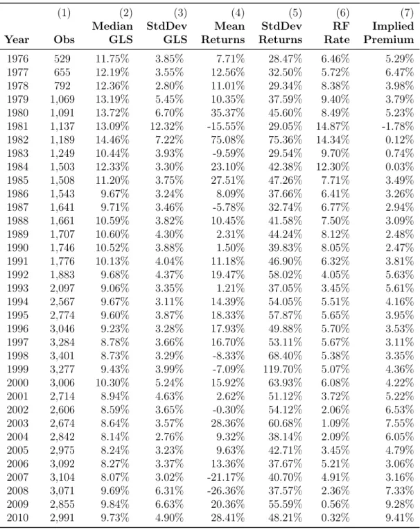
In Table 1 summary statistics on GLS in my sample are reported and contrasted with realized returns, an ex-post proxy for ex ante expected returns. Panel A reports annual cross-sectional summary statistics, including the total number of firms, the median timetexpectation of book values, net income, and dividends in t+n.
value and standard deviation of GLS, the average and standard deviation of 12-month-ahead realized returns, the risk-free rate, and the implied risk premium, computed as the difference between the median GLS and the risk-free rate. I use as the risk-free rate the one-year Treasury constant maturity rate on the last trading day in June of each year.8
Panel B reports summaries of the Panel A data by five-year sub-periods and for the entire sample period. For example, columns 2-7 of Panel B reports the averages of the annual median and standard deviation of GLS, the averages of the annual mean and standard deviation in realized returns, the average of the annual risk-free rate, and the average of the annual implied risk-premium over the relevant sub-periods.
Overall, the patterns and magnitudes shown in Table 1are consistent with prior im-plementations of GLS (e.g., Gebhardt et al., 2001). Panel B shows that, over the entire sample period the mean value of GLS (10.25%) is close to the mean value of realized returns (10.23%). But unlike realized returns, whose average cross-sectional standard deviation is 47.67%, GLS exhibits far less variation, with an average cross-sectional stan-dard deviation of 4.34%. This contrast highlights one of the widely-perceived advantages of ICCs, that it is a less noisy (i.e., lower measurement error variance) proxy for expected returns compared to ex-post realized returns; consistent with this view, a comparison of the time-series variation in columns 2 and 4 in Panel A reveals that average annual realized returns exhibits greater variability than median annual GLS.
3.2
Estimation of AR(1) Parameters
φ
iand
ψ
gls iUsing GLS, I estimate the AR(1) parameters of expected returns and measurement errors [from (5) and (6) respectively] following the methodology outlined in Appendix
A. I show that the expected-returns persistence parameter for a firm (φi), under the model dynamics, is identified by the equation cri(s+ 1) = φi ×cri(s), where cri(s) ≡
Cov ri,t+s,ber gls i,t
is the covariance between firmi’s realized annual returns fromt+s−1 to t+s and GLS in period t. The expected-returns AR(1) parameter can be estimated from the slope coefficient of an OLS regression of {crbi(s+ 1)}Ts≥1 on{crbi(s)}
T
s≥1, where
8Obtained from the website of the Federal Reserve Bank of St. Louis:
http://research. stlouisfed.org/fred2/series/DGS1/
b
cri(s) is the sample analog of cri(s). I also show that the GLS measurement-error per-sistence parameter for a firm (ψglsi ) is identified by the equation ci(s)−cri(s+ 1) =
ψi ×[ci(s−1)−cri(s)], where ci(s) ≡ Cov
b
erglsi,t+s,erbglsi,t is the s-th order sample au-tocovariance of the firm’s GLS. The measurement-error persistence parameter can be estimated from the slope coefficient of an OLS regression of {bci(s)−crbi(s+ 1)}
T s≥1 on
{bci(s−1)−crbi(s)} T
s≥1, wherebci(s) is the sample analog of ci(s).
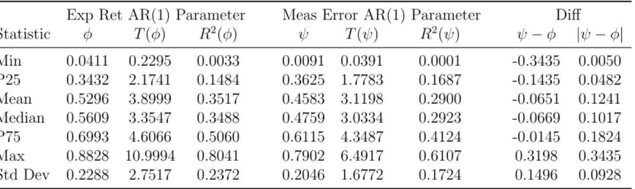
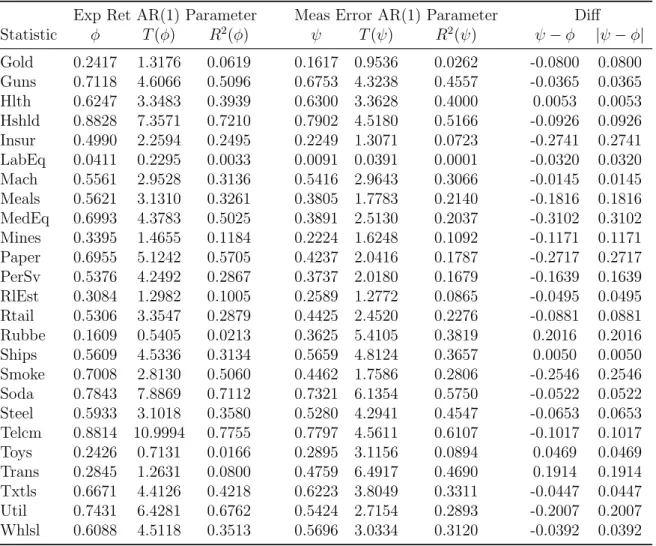
Estimates of industry-specific persistence parameters, using Fama and French (1997) 48-industry classification, are reported in Table 2. Panel B of Table 2 reports the esti-mated persistence parameters, the t-statistics, and R2 for each of the 48 Fama-French
industries (excluding the “Miscellaneous” category), and Panel A reports summary statis-tics across all industries. These estimates are produced using sample industry-specific covariances and autocovariances for up to 19 lags.9 In every industry the estimated
persistence parameters for expected returns are positive and bounded between 0 and 1, consistent with expectations and with findings in the prior literature that expected re-turns are persistent and time-varying. Across the 47 industries in the sample, the mean (median) industry AR(1) parameter for expected returns is 0.55 (0.56), with a standard deviation of 0.21, mean (median)t-statistics of 3.82 (3.35), and mean (median) R2 from
the linear fit of 36.39% (34.88%).
Table 2 also reports the first estimates, to my knowledge, of ICC measurement-error persistence in the literature. I find the measurement errors of GLS to be persistent and time-varying, but on average less persistent than expected returns. The mean (median) industry AR(1) parameter for GLS measurement errors is 0.47 (0.48), with a standard deviation of 0.18, mean (median)t-statistics of 3.05 (3.03), and mean (median) R2 from
the linear fit of 29.23% (28.93%). Finally, the last two columns of Table 2 reports the differences and absolute value of the differences between the expected returns and mea-surement error AR(1) parameters—i.e., ψbgls −φb. Panel B shows that for 38 of the 47
9For each industry l and for lags s = 1, ...,19, I estimate
b crl(s) ≡ Covd ri,t+s,berglsi,t ∀i ∈ l and b cl(s) ≡ Covd b
erglsi,t+s,erbglsi,t ∀i ∈ l. These estimated covariances, {crbl(s)} 19
s≥1 and {crbl(s)}
19 s≥1, are then used to estimate the industry-specific expected-returns and GLS measurement-error persistence parameters.
industries in the sample, this difference is negative, so that expected returns are more persistent than measurement errors; the mean (median) difference, reported in Panel A, is -0.07 (-0.08), with a standard deviation of 0.14. The last column in Panel A sum-marizes the abolute differences to give a sense of the magnitudes of the denominator in constructing wb: the mean (median) absolute difference is 0.13 (0.11), with a standard deviation of 0.09.10
With these industry-based AR(1) parameters estimates, I construct the GLS measurement-error proxy: b wglsi,t ψbglsi ,φbi ≡ erb gls i,t+1−φbi b erglsi,t b ψglsi −φbi . (15)
Using this proxy as the dependent variable, I estimate the cross-sectional associations between GLS measurement errors and firm characteristics via fixed-effects regressions, following (11).
3.3
Cross-Sectional Variation in GLS Measurement Errors
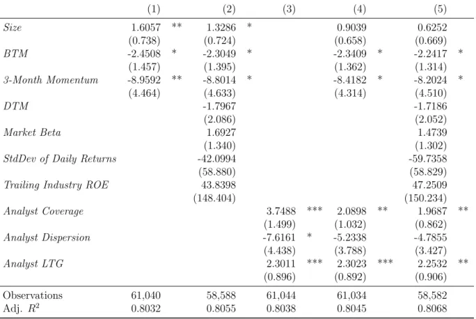
3.3.1 GLS Measurement Errors and Firm CharacteristicsTable4reports results from a pooled fixed-effects regression of the GLS measurement-error proxy,wbglsi,t, on ten firm characteristics that are commonly hypothesized explain the cross-sectional variation in expected returns and that have been widely used as explana-tory variables in the ICC literature: Size, defined as the log of market capitalization (in $millions); BTM, defined as the log ratio of book value of equity to market value of eq-uity; 3-Month Momentum, defined as a firm’s realized returns in the three months prior to June 30 of the current year; DTM, defined as the log of 1 + the ratio of long-term debt to market capitalization; Market Beta, defined as the CAPM beta and estimated for each firm on June 30 of each year by regressing the firm’s stock returns on the CRSP value-weighted index using data from 10 to 210 trading days prior to June 30; Standard Deviation of Daily Returns, defined as the standard deviation of a firm’s daily stock re-10With the exception of two industries, Healthcare and Shipbuilding, the absolute differences in AR(1) parameters exceed 0.01. Excluding these industries does not qualitatively change the empirical results of this paper.
turns using returns data from July 1 of the previous year through June 30 of the current year; Trailing Industry ROE, defined as the industry median return-on-equity using data from the most recent 10 fiscal years (minimum 5 years and excluding loss firms) and using the Fama-French 48-industry definitions; Analyst Coverage, defined as the log of the total number of analysts covering the firm; Analyst Dispersion, defined as the log of 1 + the standard deviation of FY1 analyst EPS forecasts; and Analyst LTG, defined as the median analyst projection of long-term earnings growth. All analyst-based data are reported by I/B/E/S, as of the prior date closest to June 30 of each year. Summary statistics of the main dependent and independent variables are reported in Table 3.
We include industry dummies following the estimation methodology (11) and year dummies to account for time effects. The computation of regression coefficients standard errors requires two steps. First, I account for within-industry and within-year clustering of residuals by computing two-way cluster robust standard errors (see Petersen, 2009;
Gow, Ormazabal, and Taylor, 2010), clustering by industry and year. Second, since the AR(1) parameters are estimated, I account for the additional source of variation (arising from the first-stage estimation) following the bootstrap procedure of Petrin and Train
(2003).11 All coefficients and standard errors have been multiplied by 100 for ease of
reporting, so that each coefficient can be interpreted as the expected percentage point change in GLS measurement errors associated with a 1 unit change in the covariate.
Table 4finds empirical evidence that GLS measurement errors are significantly asso-ciated with characteristics relevant to the firm’s risk and growth profile (e.g., Size,BTM, and Analyst LTG) and with characteristics relevant to the firm’s information environ-ment (e.g.,Analyst Coverage andAnalyst Dispersion). Columns 1 and 2 report a positive (negative) association betweenSize (BTM and 3-Month Momentum) and GLS measure-ment errors, but no significant associations exist with DTM, Market Beta, Standard
11The methodology adds an additional term—the incremental variance due to the first-stage estimation—to the variance of the parameters obtained from treatingφbi,ψb
gls i as the true φi, ψglsi . Specifically, I generate 1000 bootstrap samples from which to estimate 1000 bootstrap AR(1) parameters. I then re-estimate the regressions using the bootstrapped AR(1) parameters (i.e., using the 1000 new bootstrap dependent variables). Finally, the variance in regression parameter estimates from the 1000 bootstraps is added to the original (two-way cluster robust) variance estimates (which are appropriate whenφandψare observed without error). These total standard errors are reported in Table4.
Deviation of Daily Returns, orTrailing Industry ROE. Column 3 considers only analysts-based variables, and finds a negative (positive) association between Analyst Dispersion
(Analyst Coverage and Analyst LTG) and GLS measurement errors. When combining analyst and non-analyst regressors, I findSize,BTM,3-Month Momentum,Analyst Cov-erage, and Analyst LTG to be significantly associated with GLS measurement errors. In specifications that include both Size and Analyst Coverage (e.g., columns 4 and 5), the coefficients on Size and their statistical significance attenuate, compared to specifi-cations that do not include Analyst Coverage (e.g., columns 1 and 2), probably due to the relatively high correlation (72%) between Size and Analyst Coverage. Interpreting the specification in column 5, I find that, all else equal, a 1 unit increase in the firm’s
BTM (3-Month Momentum) is associated with an expected 2.24 (8.20) percentage point decrease in GLS measurement errors, with significance at the 10% (10%) level, and a 1 unit increase in a firm’s Analyst Coverage (Analyst LTG) is associated with an expected 1.97 (2.25) percentage point increase in GLS measurement errors, with significance at the 5% (5%) level. Overall, this evidence is consistent with GLS measurement errors leading to spurious correlations in regression settings.
The results of Table 4are consistent with the findings in the accounting literature on the biases in analysts’ forecasts. For example, the empirical findings that analysts tend to issue overly optimistic forecasts for growth firms (e.g., Dechow and Sloan, 1997; Frankel and Lee, 1998; Guay et al., 2011) imply that growth (lower BTM) firms tend to have higher ICCs and, all else equal, should produce more positive ICC measurement errors— consistent with the negative coefficients on BTM in Table 4. The empirical literature also finds that high LTG estimates may capture analysts’ degree of optimism (La Porta,
1996), implying that firms with high LTG projections tend to have higher ICCs and, all else equal, should produce more positive ICC measurement errors—consistent with the positive coefficients onAnalyst LTG in Table 4. However, bias in analysts’ forecasts may not be the only drivers of GLS measurement errors, since these firm characteristics (e.g., Size and BTM) can also influence measurement errors through functional form misspecification, for example through the implicit ICC assumption of constant expected
returns.12 The next section will show that both of the these sources of are important in
explaining variations in GLS measurement errors.
3.3.2 GLS Measurement Errors, Analyst Forecast Optimism, and Term Struc-ture
Whether GLS measurement errors are driven entirely by analysts’ forecast biases has important implications for the empirical solutions for improving the expected-returns proxy. This section tests the roles of analyst forecast errors and the implicit assumption of a constant expected return (Hughes et al., 2009) in driving GLS measurement errors. Ex ante, I expect ICC measurement errors (w) to be increasing with the degree of earnings-forecast optimism Eb−E. The intuition is easy to see in the dividend discount model: holding prices and fundamentals (i.e., true expected returns) fixed, an increase in forecasted cash flows (the numerator) in some future period mechanically increases the implied cost of capital (the denominator), thereby making the measurement errors—the difference between the ICC and the underlying expectation of returns—more positive. I also expect ICC measurement errors to be increasing in the slope of the term struc-ture in expected returns (i.e., a violation of the constant expected returns assumption). The ICC represents some weighted average of the expected rates of returns over time
12To illustrate, let w(x) =fb p,Eb(x), x −f(p, E, x)
where fbis a function mapping prices and forecasts of earnings to an ICC, f is the function mapping
prices and “true” expectations of earnings to “true” expected returns, andwis the measurement error. Letxbe some firm characteristic that is relevant in determining the functional forms of expected returns and ICCs, and that also affects the degree of optimism in earnings forecastsEb.
A simple first-order Taylor approximation ofwaroundx= 0 yields the following expression w≈hfb p,Eb(0),0 −f(p, E,0)i+hfbE p,Eb(0),0 b Ex(0) +fbx p,Eb(0),0 −fx(p, E,0) i x, so that the marginal effect of the firm characteristicxon measurement errors is approximated by:
w0≈fbE p,Eb(0),0 b Ex(0) + h b fx p,Eb(0),0 −fx(p, E,0) i .
This expression says that a change in the firm characteristicx affects ICC measurement errors in two ways: through its effect on the forecast of earnings (the first term on the right) and through the functional form effect (the second and third terms on the right).
It is also difficult to signw0 for some arbitrary characteristicx. WhilefbE is positive, the signs ofEbx,
b
fx, andfx are ambiguous. For any arbitrary firm characteristic, therefore, there is no clear prediction on how it will be associated with ICC measurement errors.
[P∞
j=1ωjEt(rt+j)]. To the extent that the term structure of expected returns is more
upward sloping—i.e., that expected rates of return further into the future increase the weighted average—the ICC is expected to over-state the expectation of returns over the next period [Et(rt+1)]. Thus, all else equal, ICC measurement errors are more positive
for firms with more positive-sloping term structures in expected returns.
I begin by testing the relation between GLS measurement errors and the degree of optimism in analyst forecasts; doing so requires unbiased forecasts for earnings expec-tations. For this purpose I adopt the mechanical earnings-forecast model of Hou et al.
(2012), which produces benchmark earnings forecasts in a two-step process: first, esti-mate historical relations between realized earnings and firm characteristics by running historical pooled cross-sectional regressions; second, apply the historically estimated co-efficients on current firm characteristics to compute the model-implied expectation of future earnings.13
This characteristic-based mechanical forecast model is a useful benchmark for study-ing analyst forecast optimism. Hou et al. (2012) show that these mechanical earnings forecasts closely match the consensus analyst forecasts in terms of forecast accuracy, but exhibit lower levels of forecast bias and higher levels of earnings response coefficients, suggesting that the mechanical forecasts are closer to the true expectations of earnings.14
Relatedly,So(2013) employs a very similar earnings-forecast model and finds that the me-chanical forecasts provide a useful benchmark for identifying systematic and predictable analyst forecast errors which do not appear to be reflected in stock prices.
Denoting Hou et al.’s time t mechanical forecasts of FYt+τ EPS as Ebj,t+τ, I define the following analyst optimism variables: for τ = 1,2,3, FYτ Forecast Optimism is the difference between the analyst FYτ median EPS forecast and Ebj,t+τ. A benchmark for a firm’s average long-run earnings is also necessary to obtain empirical measures for the level of optimism in the terminal earnings forecast in GLS. I use the average of 13AppendixBexplains my implementation and estimation ofHou et al.(2012)’s mechanical forecast model.
14These authors define forecast bias as realized earnings minus forecast earnings (standardized by market capitalization for model-based forecasts and by price for I/B/E/S forecasts); they define forecast accuracy as the absolute value of forecast bias.
FY3, FY4 and FY5 mechanical forecasts [i.e., (Ebj,t+3 +Ebj,t+4+Ebj,t+τ)/3] as the long-run benchmark, and define Terminal Forecast Optimism as the difference between the implied FY12 earnings and the long-run benchmark.15 Finally, following the literature,
I also create scaled versions of the optimism variables, scaling by total assets and by the standard deviation in analyst FY1 earnings forecasts.
It is worth highlighting a couple of interesting features of GLS, features that yield some intuitions about the expected relations between GLS measurement errors and ana-lyst forecast optimism and that facilitate the assessments of my empirical methodology and results. The first such feature is the important role of the FY3 earnings forecast. GLS forecasts the ratio of expected net income to expected book value from FY4 to FY11 by linearly interpolating from the forecasted FY3 ratio to the trailing industry median ROE. Holding constant the accuracy of the terminal forecast, to the extent that FY3 earnings forecasts are overly optimistic, the subsequent years’ forecasts will also be upwardly biased. Therefore, the degree of optimism in FY3 forecasts is expected to play an especially important role in explaining GLS measurement errors. A more obvious fea-ture of GLS is the important role of the terminal value assumption; all else equal, GLS measurement errors are expected to be positively associated with the degree of optimism in the terminal earnings forecast.
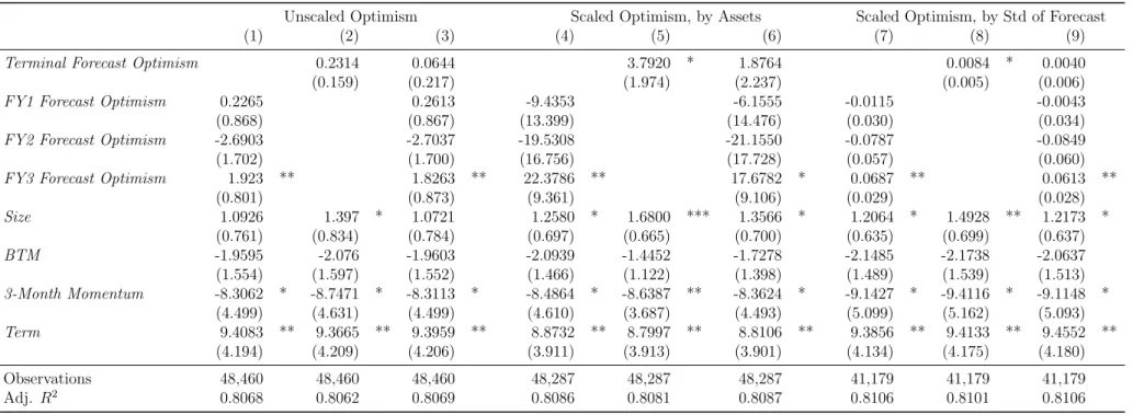
Table 5 reports results from a pooled fixed-effects regression of GLS measurement-error proxy, wbglsi,t, on FY1, FY2, and FY3 Forecast Optimism and Terminal Forecast Optimism. Year and industry fixed effects are included throughout, and the computation of standard errors as well as the reporting conventions are identical to Table4. Columns 1-3 use the unscaled optimism variables, and columns 4-6 (7-9) use the scaled optimism variables, scaling by total assets [standard deviation of FY1 analyst forecasts]. Consis-tent with intuition, GLS measurement errors are associated positively and significantly (at the 1% level) withFY3 Forecast Optimism (columns 1, 4, and 7), and positively and 15The use of the average of FY3, FY4, and FY5 as a benchmark need not follow from the assump-tion that such an average represents a good levels forecast of the firm’s long-run earnings. Under the assumption that the difference between the GLS terminal EPS forecast and the long-run benchmark is proportional to the difference between the GLS terminal EPS forecast and the true but unobserved expected long-run EPS, variations in Terminal Forecast Optimism may still be informative about the degree of terminal forecast optimism.
significantly (at the 5% level) with Terminal Forecast Optimism (columns 2, 5, and 8), regardless of scaling.16 In specifications that include all optimism variables (columns 3,
6, and 9),FY3 Forecast Optimism appears to be more important in explaining measure-ment errors, as its coefficient remains associated positively and significantly (at the 5% level) with GLS measurement errors, while the coefficient onTerminal Forecast Optimism
is attenuated and no longer statistically significant at conventional levels. Interpreting the coefficients in column 3, I find that a one dollar increase in analysts’ FY3 Forecast Optimism is associated with an expected 1.14 percentage-point increase in GLS mea-surement errors, with statistical significance at the 5% level; a one dollar increase in
Terminal Forecast Optimism is associated with an expected 22 basis-point increase in GLS measurement errors, but the coefficient is not statistically significant at the conven-tional levels. Measures of FY1 and FY2 Forecast Optimism are not significant in any of the specifications in Table 5, which is unsurprising in that for GLS the bias in FY3 earnings forecasts has disproportionate influence on GLS measurement errors.
Table 6 considers jointly the influence of analyst forecast optimism and the implicit assumption of constant expected returns on GLS measurement errors. In particular, I use a proxy from the work of Lyle and Wang (2013), who develop a methodology for estimating the term structure of expected returns at the firm level based on two firm fundamentals: BTM andROE. Their model assumes that the expected quarterly-returns and the expected quarterly-ROE revert to a long-run mean following AR(1) processes, and produces empirical estimates of a firm’s expected returns over all future quarters. I approximate the slope of the term structure (Term) as the difference between the long-run expected (quarterly) returns from the expected one-quarter-ahead returns following the model ofLyle and Wang (2013).
Table 6 replicates the fixed-effects regressions of Table 5, but includes as additional controls Size, BTM, 3-Month Momentum, and Term. Qualitatively the results with re-spect to analyst forecast optimism remain unchanged, but the coefficients and their sta-tistical significance attenuate slightly relative to Table 4. The attenuation is probably 16In untabulated results, I find that scaling forecasts by price yields qualitatively identical results to those of Table5.
due to the partial capture of analyst optimism by the controls—for example, the afore-mentioned empirical observation that analysts are overly optimistic about higher-growth (e.g., lower BTM) firms. Moreover, I find consistent evidence that the constant term structure assumption is important in driving GLS measurement errors. In all specifica-tions, the steeper the slope in the term structure of expected returns, the more positive are GLS measurement errors, with all coefficients on Term being statistically significant at the 5% level.
The results of Table 5 are consistent with the intuition built on an understanding of GLS’s unique features, and these results provide evidence that the methodology devel-oped in this paper are useful for explaining the variations in GLS measurement errors. Table 5suggests that optimism in analyst FY3 forecasts, optimism in the terminal earn-ings forecasts, and the constant expected return assumption are significant drivers of GLS measurement errors. However, FY3 Forecast Optimism appears to have a greater influence thanTerminal Forecast Optimism, both in the magnitude of its association and in its statistical significance.17 To my knowledge, the empirical results of Tables4–6 are the first direct empirical evidence broadly in support of the theoretical results of Hughes et al. (2009).
3.3.3 Sorting Future Returns
A potential concern with interpretation of the preceding results is that the regression coefficients (e.g., Table 4) could be driven by the measurement errors in the estimates of GLS measurement errors. Though these concerns are mitigated by Tables 5 and 6
that report results consistent with one’s intuition about the sources of GLS measure-ment errors, this section reports on further tests showing that the empirical methodology presented in this paper is informative about GLS measurement errors.
Section 2.3 shows that if wbi,tgls is indeed informative about GLS measurement errors’ cross-sectional associations with firm characteristics, then a modified version of GLS (erbmglsi,t ≡ erbglsi,t −wbglsi,t) is informative about the cross-sectional association between ex-17This may be due to the possibility that earnings forecast optimism can be measured with greater precision in the short run than in the long run.
pected returns and firm characteristics. In particular, if the paper’s model is valid for GLS, then a fixed-effects regression of Modified GLS (ModGLS) on firm characteristics produces regression coefficients that better capture the systematic associations between expected returns and firm characteristics than regressions using GLS. To test this pre-diction, I construct proxies of expected returns using historically estimated regression coefficients on firm characteristics estimated using ModGLS, and compare them with similarly estimated expected return proxies but estimated using GLS. I expect those proxies constructed from historically estimated associations between ModGLS and firm characteristics to exhibit a greater ability to sort future returns.
I follow a two step procedure to create expected return proxies using historically estimated associations between ModGLS and firm characteristics. First, in each year (t) regress ModGLS on firm characteristics using three years’ data fromt−1 to t−3 (with year and industry fixed effects), and obtain estimated coefficients bδt−1.18 Second, apply
the coefficientsbδt−1 on current values of covariatesXt to obtain expected returns (Fitted ModGLS) over the next year.
I consider three sets of covariates (corresponding to the significant covariates in the three regression specifications of Table 9 presented in the next section). Model 1 is a three-factor model with
Xt={Sizet, BTMt, M omentumt};
Model 2 is a five-factor model with
Xt={Sizet, BTMt,M omentumt,DTMt, StdRett};
and Model 3 is an seven-factor model with
Xt={Sizet,BTMt, M omentumt,DTMt, StdRett, AnalystDispersiont, AnalystLT Gt}.19
18The regression requires a 1-year lag since the dependent variable,
b
ermglsi,t ≡ berglsi,t −wbi,t
b
ψigls,φb
, requiresbermglsi,t+1. Recall thatwbi,t
b ψigls,φb =ber gls i,t+1−φibber gls i,t b ψglsi −φib .
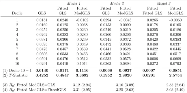
After estimating the Fitted ModGLS using this procedure, I sort them into decile port-folios and summarize the average realized 12-month-ahead returns within each decile. I compare these average returns to those produced by decile portfolios formed by GLS (i.e., by decile ranking erbglsi,t) and Fitted GLS, which is created following the above two-step procedure but using GLS as the dependent variable. Again, if the regression coefficients estimated using ModGLS better capture the systematic relations between expected re-turns and firm characteristics, then I expect Fitted ModGLS to sort future rere-turns better than does Fitted GLS. As a performance metric, I compare the average decile spread— i.e., the average difference in the realized 12-month-ahead returns between the top and bottom decile portfolios—over the period from June 30, 1979 to June 30, 2010.20
Table 7 Panel A (B) compares the realized 12-month-ahead market-adjusted (size-adjusted) returns between GLS, Fitted GLS, and Fitted ModGLS decile portfolios, which are formed annually.21 The Fitted ModGLS sorts future returns best, producing substan-tially larger decile spreads (reported in row 1) than either GLS or Fitted GLS. Panel A (B) finds the average market-adjusted (size-adjusted) annual decile spread for GLS to be 1.4% (-0.30%), with time-series t-statistic of 0.43 (-0.95), suggesting that those firms with the highest values of GLS do not on average have realized returns that are statisti-cally different from those with the lowest values of GLS.22 Similarly, in none of the three
models does Fitted GLS exhibit significant ability to sort future market- or size-adjusted returns.
In contrast, Fitted ModGLS exhibits economically and statistically significant ability to sort future returns in each of the three models. Fitted ModGLS estimated usingModel 1,2, and3 produces average decile spreads in market-adjusted (size-adjusted) returns of 11.16% (9.23%), 9.37% (7.58%), and 8.51% (6.69%), with all spreads statistically different from 0% at the conventional levels. Finally, tests of the hypotheses that the decile spreads even though in Table9 the coefficients onAnalyst Coverage are significant.
20The first year for which I obtain Fitted ModGLS estimates is 1979, since our overall sample begins in 1976 and obtaining Fitted ModGLS estimates requires data from 1976 to 1978.
21Market adjustment is performed using the value-weighted CRSP market index; size adjustments are performed using CRSP size deciles, formed at the beginning of each calendar year.
22Time-series t-statistics are computed using the time-series standard deviation of annual decile spreads.
produced by Fitted ModGLS are no different from those produced by GLS (reported in row 3) or Fitted GLS (reported in row 4) are rejected at the conventional levels in all cases, whether using a standard t-test or the Wilcoxon signed-rank test, suggesting that Fitted ModGLS exhibits superior return-sorting ability.
Table8repeats the exercise presented in Table7, but considers decile portfolios formed within each year and each Fama-French industry. In other words, Table 7 compared the relative performance of GLS, Fitted GLS, and Fitted ModGLS in sorting future returns for the cross-section of stocks; Table 8 compares how they sort within-industry returns. Overall the results of Table 8 are consistent with those of Table 7. GLS and Fitted GLS exhibit no economically or statistically significant within-industry sorting ability. In contrast, Fitted ModGLS exhibits significant within-industry return-sorting ability in each of the three models, with decile spreads that are economically and statistically significant and that are statistically different from those produced by GLS or Fitted GLS. In summary, the results of Tables 7 and 8 support the hypothesis that the methodology developed in this paper is informative about GLS measurement errors and provides empirical evidence that regressions using Modified GLS produce coefficients that better capture the systematic relations between expected returns and firm characteristics.
3.4
Expected Returns and Firm Characteristics
Having established the efficacy of this paper’s methodology in explaining GLS mea-surement errors, I will now assess the quality of inferences about the associations between expected returns and firm characteristics in regressions using GLS. In Table 9Panels A, B, and C, I estimate fixed-effects regressions of expected return proxies on firm char-acteristics widely hypothesized to be associated with the expected rate of returns. For ease of interpretation, I follow Gebhardt et al. (2001) and standardize each explanatory variable by its cross-sectional annual mean and standard deviation. Year and industry fixed effects are included in each regression and the reporting conventions are as specified in Table 4.
using GLS and ModGLS, respectively. In keeping with the model proposed in this paper and by the evidence reported from Tables4–8, regressions using ModGLS should be more informative about the systematic relations between expected returns and firm character-istics than regressions using GLS. Panel A considersSize,BTM, and3-Month Momentum
as covariates, as in Model 1 of Tables 7 and 8. Consistent with expectations from prior literature, I find in Panel A, column 1 a negative (positive) association between GLS andSize (BTM), with the coefficients being statistically significant at the 1% (1%) level. Unexpectedly, the association between GLS and 3-Month Momentum is negative and statistically significant at the 1% level, which is inconsistent with the well-documented momentum effect (e.g., Jegadeesh and Titman, 1993; Chan, Jegadeesh, and Lakonishok,
1996) that would predict a positive coefficient. The negative association between GLS and momentum is probably an artifact of how GLS (and ICCs more generally) is constructed. Since price and erbglsi,t are inversely related by construction (14), holding expectations of future fundamentals fixed, firms with greater recent price appreciation may also tend to have lower values of GLS.
Column 2 of Panel A estimates fixed-effects regression coefficients of ModGLS onSize,
BTM, and3-Month Momentum. The coefficients onSize and BTM remain negative and positive, respectively, similar to the column 1 results using GLS, though the estimated magnitudes differ. In contrast, the coefficient on 3-Month Momentum reverses in sign: it is positive and statistically significant at the 10% level, consistent with predictions of the momentum phenomenon. Consistent with the empirical evidence in Table 4, that GLS measurement errors are more negative for higher momentum firms, the negative and significant coefficients on3-Month Momentum in column 1 probably captureMomentum’s associations with GLS measurement errors.
Table9, Panel B adds four more firm characteristics to the covariates of Panel A: Mar-ket Beta,DTM,StdDev of Daily Returns, andTrailing Industry ROE. In column 1, using GLS as the dependent variable, the coefficients on Size, BTM, and 3-Month Momentum
are very similar to those reported in Panel A, column 1 in terms of both magnitudes and statistical significance. Moreover, GLS is associated negatively and significantly (at
the 1% level) with Market Beta, and positively and significantly with DTM, StdDev of Daily Returns, and Trailing Industry ROE (all at the 1% level). The results on Market Beta andTrailing Industry ROE are unexpected. If CAPM were true, I would expect the relation between expected returns and Beta to be positive; if CAPM does not describe the cross-sectional variation in expected returns, or if the estimation ofBeta is too noisy, I expect no association with expected returns. It is also unclear whether a positive as-sociation should exist between a firm’s expected returns and its Trailing Industry ROE. This is probably a mechanical artifact of the way GLS is constructed. Since GLS uses the Trailing Industry ROE in its terminal value assumptions, higher Trailing Industry ROE mechanically yields higher values of GLS, all else equal.
Panel B, column 2, which uses ModGLS as the dependent variable, also shows that the inclusion of the four additional variables has little impact on the coefficients on
Size, BTM, and 3-Month Momentum: all three coefficients remain very similar to those reported in Panel A, column 2, in terms of both magnitudes and statistical significance. As in Panel A, the coefficient on 3-Month Momentum reverses in sign, from negative and significant in column 1 to positive and significant in column 2. Moreover, Panel B, column 2, reports coefficients onDTM andStdDev of Daily Returns that are positive and significant, consistent both with expectations and with column 1. Unlike in column 1, the coefficient onMarket Beta is no longer statistically different from 0, though its magnitude is larger; nor is the coefficient onTrailing Industry ROE any longer statistically different from 0, with magnitudes that are substantially attenuated toward zero. This evidence, combined with the results of Table 4, suggests that the associations of GLS with Beta
andTrailing Industry ROE are probably influenced by systematic measurement errors in GLS.
Table 9, Panel C, adds to the covariates in Panel B three analyst-based variables:
Analyst Coverage,Analyst Dispersion, andAnalyst LTG. The addition of these variables does not substantially change the magnitudes or significance of the coefficients on the non-analyst variables in column (1) compared to Panel A. Moreover, I find that GLS is positively and signficantly (at the 1% level) associated with Analyst Dispersion and
Analyst LTG. The coefficient on Analyst Coverage is negative, but not statistically dif-ferent from 0, probably due to collinearity between Size and Analyst Coverage. The positive association between GLS and Analyst LTG is unexpected and inconsistent with the empirical observation that firms with high LTG estimates tend on average to have lower returns (e.g., La Porta, 1996). This positive association is probably a mechanical artifact of how GLS is calculated. Recall that GLS uses median analyst forecasts of FY1, FY2, and FY3 EPS; however, the FY3 forecast is imputed by applying Analyst LTG
projections to the median FY2 EPS forecast. To the extent that larger values ofAnalyst LTG tend to be too extreme, as argued by La Porta (1996), GLS’s forecasts of FY3 earnings will also be too optimistic. In other words, the positive association between GLS andAnalyst LTG probably reflects the degree of optimism in FY3 forecasts.23 With
the exception ofSize, the addition of analyst variables in Panel C does not substantially change the magnitudes or significance of the coefficients on the non-analyst variables in column 2 relative to those in Panel A. The attenuation in the coefficient and significance of Size is not surprising, given the relatively high correlation (72%) between Analyst Coverage andSize. Consistent with column 1, I find ModGLS to be associated positively and significantly (at the 1% level) with Analyst Dispersion; however, unlike column 1 and consistent with expectations, the coefficient on Analyst LTG reverses in sign and becomes negative and statistically significant at the 5% level. This evidence, combined with the results of Table4, suggest that the associations between GLS and Analyst LTG
are probably influenced by systematic measurement errors in GLS.
A natural question arising from the above results—that GLS likely suffers from spuri-ous correlations through dependent-variable measurement errors—is whether mitigating earnings-forecast biases could improve regression inferences. The results of Tables5and6
suggest that earnings-forecast optimism is not the sole driver of GLS measurement errors; column 3 of each panel in Table 9addresses this question explicitly. Specifically, column 3 uses as the dependent variable MechGLS, another proxy of expected returns that imple-ments GLS but uses the benchmark earnings forecasts ofHou et al.(2012). In general, the 23In untabulated results, I find that the measures ofFY3 Forecast Optimism used in this paper are positively and significantly associated withAnalyst LTG.
regression coefficients using MechGLS are directionally similar to those estimated using GLS, but the magnitudes and statistical significance may differ. In all three panels, for example, the coefficients on Size and BTM are substantially larger in magnitude than those estimated using GLS, and generally closer to the coefficients on Size and BTM
reported in column 2. Many of the surprising coefficients estimated using GLS persist in regressions using MechGLS: 3-Month Momentum and Market Beta remain negative and significant (both at the 1% level), whileTrailing Industry ROE remains positive and significant (at the 1% level) in all relevant panels. Interestingly, in Panel C, column 3, the association between MechGLS and Analyst LTG is negative, reversing in sign from column (1), though the coefficient is not statistically different from 0 at the conventional levels. In summary, MechGLS appears to resolves some puzzling associations between GLS and firm characteristics, but many of the unexpected associations persist, consistent with the view that the spurious correlations between firm characteristics and GLS mea-surement errors do arise solely from analysts’ earnings-forecast errors; they could also be due to errors arising from functional form assumptions.
Finally, in Table9, column 4 of each panel estimates regressions using 12-month-ahead realized returns as an ex-post proxy for expected returns. Realized returns is defined as the sum of expected returns and news (see, e.g., Campbell, 1991; Vuolteenaho, 2002). The latter component represents realized returns’ errors in measuring ex ante expected returns, but these measurement errors (i.e., “news”) have some advantageous proper-ties. Realized returns provide unbiased estimates of expected returns since, as Lewellen
(2010) notes, the latter is defined as the expectation of realized returns conditional on information known prior to the period. Thus the measurement errors of realized returns have zero mean and, by the definition of news, cannot be systematically predictable. With a sufficiently long panel dataset, regressions of realized returns are not expected to be influenced by spurious correlations via dependent-variable measurement errors. The disadvantage of using realized returns stems from the high variance in its measurement errors (both in the cross section and in time series), which is consistent with the sub-stantially larger cross-sectional and time-series standard deviations compared to those of
GLS, as shown by comparing average values of columns 3 and 5 in Table1, Panel A, and by comparing the variability of columns 2 and 4 in Table1, Panel A. Thus, compared to GLS, the use of realized returns is expected to reduce the precision with which researchers can estimate associations between expected returns and firm characteristics.
Comparing the regression coefficients estimated using realized returns to those that use alternative proxies of expected returns, I find that the coefficients in column 4 align most closely in terms of sign, magnitude, and statististical significance with those in column 2 estimated using ModGLS. Like column 2, column 4 finds a positive and significant coefficient on3-Month Momentum across all three panels, and no statistical significance in the coefficients on Market Beta and Trailing Industry ROE. However, regressions of realized returns in Panels B and C do not obtain statistical significance in DTM, StdDev of Daily Returns,Analyst Dispersion, or Analyst LTG, though these coefficients have the same signs as in column 2.
Overall, the estimates in column 4 help bolster the hypothesis that regression coeffi-cients estimated using GLS (or MechGLS) are influenced by spurious correlations with the dependent variable’s measurement errors, and that the problem is unlikely to be fully resolved by accounting for systematic earnings-forecast biases. Given the results of Table
9and the puzzling associations between GLS and certain firm characteristics, it is unsur-prising that regression coefficients estimated using ModGLS produce proxies of expected returns that exhibit superior return-sorting ability in Tables 7 and 8.
4
Summary, Implications, and Conclusion
This paper presents a methodology for assessing the cross-sectional associations be-tween measurement errors in expected-return proxies and firm characteristics, and a methodology for making inferences about expected returns in light of such systematic measurement errors. I show that the paper’s methodology is useful in explaining measure-ment errors of GLS, one of the most popular implemeasure-mentations of ICCs, and I documeasure-ment several findings contributing to the ICC literature. The paper reports the first empirical
evidence that ICC measurement errors are persistent and time-varying, and that GLS measurement errors are systematically associated with certain firm characteristics com-monly assumed to be associated with expected returns. Finally, I find evidence that many unexpected associations between GLS and firm characteristics, such as 3-Month Momentum,Market Beta, Trailing Industry ROE, andAnalyst LTG, are likely driven by spurious correlations with dependent variable measurement errors rather than underlying economics.
These empirical findings have three important practical implications for researchers who use ICCs as proxies for expected returns. First, regression results reliant on cross-sectional regressions of ICCs on firm characteristics may be influenced by spurious asso-ciations with dependent-variable measurement errors. This observation may explain such puzzling associations as the negative association between ICCs and momentum (e.g.,
Guay et al.,2011) and the positive association between ICCs and trailing industry ROE (e.g., Gebhardt et al., 2001).
This implication also raises questions about the efficacy of assessing the quality of ICCs by comparing the associations between firms’ risk characteristics and ICCs (e.g.,Botosan and Plumlee, 2005; Botosan, Plumlee, and Wen, 2011) in regression settings. To the extent that regression coefficients reflect spurious correlations between ICC measurement errors and risk characteristics, it is unclear whether or why ICCs that exhibit stronger associations with presumed risk characteristics are necessarily better. For example, ICCs whose measurement errors are strongly correlated with characteristics such as Size and
BTM need not be better proxies of expected returns; to make such an assessment requires further definition of the researcher’s preferences over ICC measurement-error properties. Second, the empirical results documented in this paper suggest that standard methods for addressing measurement errors, namely portfolio grouping and instrumental variables, may have limited effectiveness. The idea behind grouping is to form portfolios of firms with similar expected returns, so that measurement errors (presumed to be random) cancel out on average at the portfolio level. Ideally, groups should be formed to minimize the within-group variation and maximize the across-group variation in expected returns.