Forecasting Precipitation Using SARIMA Model: A Case Study of
Mt. Kenya Region
Hellen W. Kibunja1*, John M. Kihoro1, 2, George O. Orwa3, Walter O. Yodah4
1. School of Mathematical Sciences, Jomo Kenyatta University of Agriculture and Technology P.O. Box 62000-00200, Nairobi, Kenya
2. Co-operative University College of Kenya, Computing and E-learning P.O. Box 24814-00502, Nairobi, Kenya
*
E-MAIL: [email protected]
Abstract
Precipitation estimates are an important component of water resources applications, example, in designing drainage system and irrigation. The amount of rainfall in Kenya fluctuates from year to year causing it to be very hard to predict it through empirical observations of the atmosphere alone. Our objective was to determine the forecasted values of precipitation in Mt. Kenya region and also to determine the accuracy of the SARIMA model in forecasting precipitation in the same region. This research considers a univariate time series model to forecast precipitation in Mt. Kenya region. We fitted the SARIMA model to our data and we picked the model which exhibited the least AIC and BIC values. Finally, we forecasted our data after following the three Box-Jenkins methodologies, that is, model identification, estimation of parameters and diagnostic check. Having three tentative models, the best model had two highly significant variables, a constant and with p-values< 0.01 respectively. This model passed residual normality test and the forecasting evaluation statistics shows ME= -0.0053687, MSE=0.96794, RMSE=0.98384 and MAE= 0.75197. Indeed, SARIMA model is a good model for forecasting precipitation in Mt. Kenya region
Keywords: SARIMA, Precipitation, Forecast, Mt. Kenya, AIC and BIC
1.0 Introduction
Time series methods determines future trend based on past values and corresponding errors. Since a time series method only require the historical data, it is widely used to develop predictive models. A time series is simply a set of observations measured at successive points in time or over successive periods of time. Time series analysis is used to detect patterns of change in statistical information over regular interval of time. These patterns are projected to arrive at an estimate for the future. Time series forecasting methods are based on analysis of historical data. It makes the assumption that past patterns in data can be used to forecast future data points. Several methods have been used in forecasting weather. We have Non parametric Methods like the Artificial Neural Networks and parametric Methods. Some of the models under parametric are: Extrapolation of trend curves, Exponential smoothing, The Holt-Winters forecasting procedure and Box Jenkins procedure.
1.2Background Information
Precipitation estimates are an important component of water resources applications, example, in designing drainage system and irrigation. Major sectors of economy in Kenya such as agriculture, livestock keeping, hydro-energy generation, transport, tourism, among others are highly dependent on climate. Severe weather and extreme climate events and other climatic fluctuations have been shown to have a high influence on the social
and economic activities of the country and the performance of the country’s economy KMD (2009). It has also been noted that the past development projects may not have taken into consideration the potential impacts that the climate has on their success. Due to the failures associated with lack of timely and effective forecasts, the agricultural activities in the country have been immensely affected causing massive losses to farmers who would have easily avoided these outcomes with prior notice; integration of technology in agriculture have brought with it crops that are rainfall specific. Traditionally, long rains occur from March through to May and short rains from October to December but because of climatic changes, this trend is somehow changing. These changes normally occur on aspects of weather such as wind speed, humidity, temperature , precipitation which occurs in a variety of forms; hail, rain, freezing rain, sleet or snow among others. Therefore, there is need more accurate forecasting techniques to be applied in predicting climatic patterns. Precipitation estimates being an important component of water resources applications, an accurate estimate of rainfall is needed. There are also concerns with producing valid estimates using appropriate methods. In order to develop a comprehensive solution to the forecasting problem, including addressing the issue of uncertainty in predictions, a statistical model must be developed.
2.0 Literature Review
Rainfall prediction is a challenging task especially in the modern world where we are facing the major environmental problem of global warming which has rendered the previously employed methods to redundant. Earlier forecasting methods such as simple quantitative precipitation forecasts used by Klein and Lewis (1970),Glahn and Lowry (1972) and Pankratz, 1983 have lost their edge due to the changing patterns and variability in rainfall that may be associated with global warming. However, the world of statistics has been evolving over time leading to creation of more efficient and effective methods allowing researchers to make enormous efforts in addressing the issue of accurate precipitation predictability. Borlando et al., 1996 used ARIMA models to forecast hourly precipitation in the time of their fall and the amounts obtained were compared with the data to measure rain. They came to the conclusion that with increasing duration of rainfall, the predictions were more accurate, and shorter duration of rainfall, rain rate difference will be more than the actual corresponding value. Yusof and Kane, 2012 analyzed the precipitation forecast using SARIMA model in Golastan province and found the seasonality measure in SARIMA to be highly useful in measuring precipitation.
2.1 SARIMA Models theory
Box Jenkins (1970) generalize ARIMA model to deal with seasonality. Autoregressive Integrated Moving Average (ARIMA) models are generalizations of a simple AR model that uses three tools for modeling serial correlation in disturbance. The first tool is an autoregressive, or AR term. Each AR term corresponds to the use of lagged value of the residual in forecasting equation for the unconditional residual. The AR model of order p, AR (p) has the following form:
= + + ⋯ + + ……… (1)
With the use of a lag operator B, the equation becomes:
1 − − − ⋯ − = = ………..(2)
Where for B holds =
Next tool is integration of order term. Each integration order corresponds to the differentiation of the series being forecast. The first order differentiation component means that the forecasting model is designed for the first difference of the original series .The second order component corresponds to the second difference and so on. The third tool is a Moving Average, MA term. The MA forecasting model uses lagged values of a forecast error to improve the current forecast. The first order MA term uses the most recent forecast error. The second
term uses the forecast error from two most recent periods and so on. MA process of order q, MA (q) has the form: It is written as
= − − ⋯ − ……… (3)
Using lag operator,
= 1 − − ⋯ − = ……….. (4)
When modeling time series with systematic seasonal movements, Box-Jenkins recommended the use of seasonal autoregressive (SAR) and seasonal moving average (SMA) terms. The seasonal autoregressive process of order P can be written as:
= Φ + Φ + ⋯ + Φ + ……….. (5)
Or
Φ = ……… (6)
The seasonal MA of order Q can be written as
= − Θ − ⋯ − Θ ……… (7)
Or equivalently,
= Θ ……….. (8)
In all the four components above, s denotes the length of seasonality. Finally, we can write the general SARIMA , , × !, ", # $with constant model as
Φ 1 − % 1 − & =
'+ Θ ……… (9)
Where the constant equals
'= ([ 1 − − − ⋯ − 1 − Φ −Φ − ⋯ − Φ ] ……… (10) 3.0 Materials and Methods
3.1 Study Area
The study concentrated on statistical modeling of precipitation in Mt. Kenya region in central Kenya. This region is predominantly agricultural dependent; its profitability would significantly increase if there was access to reliable and timely forecast of rainfall data. This region would benefit from the success of this study. The region also has other sectors that depend on reliable forecasts of climatic conditions such as tourism, some service industry such as electricity and water supply. Mount Kenya region is the source of major rivers in Kenya and the climatic conditions in this area are highly unpredictable.
3.2 Study Data
The data employed in this research comprises precipitation and wind monthly data collected from Kenya meteorological department covering a period of 1995 to 2010 for wind data and 1970 to 2011 for precipitation data but will be limited to the available wind data. This data is highly reliable as it is collected on a daily basis in the stations and therefore future data needs may be easily met from the station.
4.0 Results
4.1 Data Analysis Process
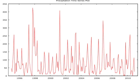
Data was analysed using Gretl which has inbuilt functions like MLE to deal with ARIMA models. Preliminary data analysis was performed on hourly daily precipitation from 1995-2010 using Box-Jenkins modeling methodology. Time series plot was done using raw data to assess the stability of the data and the following time series plot was obtained.
4.2 Precipitation Time Series Plot
Figure 1 plot show that our data is stationary. A non stationary series is the one in whose values do not vary with time over a constant mean and variance.
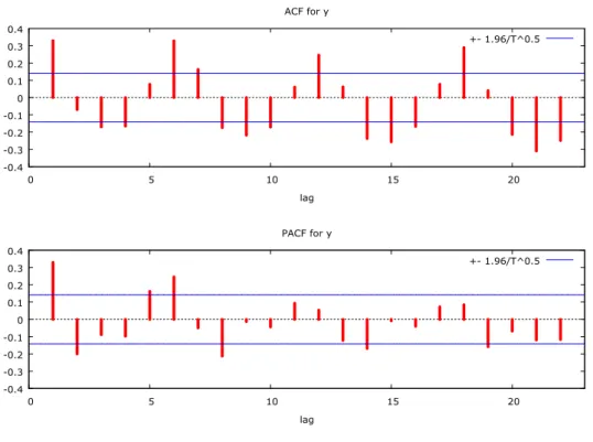
4.3 ACF and PACF plots of precipitation
Figure 2 show ACF and PACF plots of precipitation. The auto-correlation indicates that there is no seasonality. Seasonality normally causes the data to be non-stationary the average values because the average values at some particular times are different than the average values at other time
4.4 SARIMA Forecasting Results
SARIMA model was fitted after following Box-Jenkins four major steps in modeling time series and the appropriate model was obtained by choosing the model which yielded minimum AIC and BIC, Akaike (1979). After a series of model tests, the following models were obtained.
4.4.1 Tentative seasonal ARIMA models
There were three tentative models as shown in table 1.
SARIMA (1, 0, 1) × (1, 0, 0)12 turns out to be the best model since it has the least values of the information criterions. The details of this model are shown in table 2. This model has two significant variables. The correlation matrix of this model was examined. The correlation between the parameters of the model was a weaker one. This implies that all the parameters are important in fitting the model. The fitted model is given by:
+ +Φ + Φ = + + + ………. (11)
Upon replacing the coefficients of the model with real values, we get the follow:
+ 0.204 + 0.464 + 0.095 = 3.84 + + + 0.117+ ……….. (12)
4.4.2ACF and PACF plots of residuals
Figure 3 show that the residuals are white noise as there are no significant spikes.
4.4.2 Normality test of residuals
Figure 4 show a histogram which has a bell shaped distribution with a p-value of 0.007 which is a good indicator of normality in the distribution.
4.4.3 Residual Q-Q Plot
The QQ plot in figure 5 approximately follows the QQ line visible on the plot. This is a good indicator of normality within the residuals
5.0 Conclusion
The main objective of this study was to forecast precipitation using SARIMA model and also to determine the accuracy of the SARIMA model in forecasting precipitation in Mt. Kenya region To avoid fitting over parametized model, AIC and BIC were employed in selecting the best model. The model with a minimum value of these information criterions is considered as the best (Akaike (1979); Akaike (1974)). In addition, ME, MSE, RMSE, MAE, MPE, MAPE were also employed. The ACF plots of the residuals two models were examined to see whether the residuals of the model were white noise. SARIMA model turns to be a good model for forecasting precipitation in Mt. Kenya region.
References
[1] Akaike Hirotugu (1974),’A New Look at the Statistical Model Identification, IEEE, Transction Automatic Control 19(6), 716.
[2] Akaike Hirotugu (1979),’Bayesian Extension of Minimum AIC Procedure of Autoregressive Model Fitting’,
Biometrika 66(2), 237-242.
[3] Anderson Oliver D. (1977), ‘Time Series Analysis and Forecasting: Another Look at the Box-Jenkins Approach’,Journal of Royal Statistical Society (The Statistician)26(4), 285-353
[4] Borlando P. ,Montana R. and Raze (1996), ‘Forecasting Hourly Precipitation in time of fall using ARIMA Models’ Journal of Atmospheric Research 42(1), 199-216.
[5] Box George Edward Pelham and Gwilyn M. Jenkins (1976), ‘Time Series Analysis; Forecasting and Control’,
Holden-Day, San Fransisco.
[6] Box George Edward Pelham, Gwilyn M. Jenkins and Reinsel G. C. (1976), ‘Time Series Analysis; Forecasting and Control’, Holden-Day, San Fransisco (3).
[7] Chatfield Chris (2004),’The Analysis of Time Series: An Introduction’, John Wiley & Sons, NewYork, U.S.
3(1),69-71
[8] Glahn Harry R. and Dale A. Lowry (1972), ‘The Use of Model Output Statistics MOS in Objective Weather Forecasting’, Journal of Applied Meteorology11, 1203-121.
[9]Klein William H. and Frank Lewis (1970),’Computer Forecasts of Maximum and Minimum Temperature’,
Journal of Applied Meteorology 9,350-359.
[10]Kenya Meteorological Department, KMD (2009), Kenya Outlook for the March-May 2011”long rains” Season’, Ministry of Environment and Mineral Resources.
[11]Pankratz Allan(1983),’Forecasting with Univariate Box-Jenkins Concept and Cases’, John Wiley & Sons, Inc. New York 78(1), 684-709.
[12] Stock J. H. and Watson M. W. (1998), ‘Forecasting in Dynamic Factors Models Subject to Structural Instability’, National Bureau of Economic Research 6(2), 98-102.
[13] George C. Tiao and Box G. E. P. (1975),’Intervention Analysis with Applications to Economic and Enviromental Problems’, Journal of the American Statistical Association,70(349), 70-79.
[14]Fadhilah Yusof and Ibrahim Lawal Kane (2012), ‘Modeling Monthly Rainfall Time Series Using ETS and SARIMA Models’, International Journal of Current Research 4(1), 195-200.
APPENDIX
AIC BIC
ARIMA (1,0,1)×(0,0,0)12 586.16 599.17
ARIMA (1,0,1)×(0,0,1)12 563.66 579.93
ARIMA (1,0,1)×(1,0,0)12 547.46 563.72
Table1: Seasonal ARIMA models
Coeff. Std. error z p-value
Const. 3.843 0.1753 21.91 1.99e-106***
0.2039 0.1828 1.116 0.2645
Φ 0.4641 0.0670 6.924 4.38e-012***
0.1171 0.1806 0.6486 0.5166
Table2: SARIMA model Performance Statistics ME -0.0053687 MSE 0.96794 RMSE 0.98384 MAE 0.75197 AIC 549.2842 BIC 565.5717
Table 3: performance Statistics
Figure 1:Precipitation Time Series Plot
0 50 100 150 200 250 300 350 400 450 1996 1998 2000 2002 2004 2006 2008 2010 y
Figure 2: ACF and PACF plots of Precipitation
Figure 3: ACF and PACF plots of residuals
-0.4 -0.3 -0.2 -0.1 0 0.1 0.2 0.3 0.4 0 5 10 15 20 lag ACF for y +- 1.96/T^0.5 -0.4 -0.3 -0.2 -0.1 0 0.1 0.2 0.3 0.4 0 5 10 15 20 lag PACF for y +- 1.96/T^0.5 -0.25 -0.2 -0.15 -0.1 -0.05 0 0.05 0.1 0.15 0.2 0.25 0 5 10 15 20 lag Residual ACF +- 1.96/T^0.5 -0.25 -0.2 -0.15 -0.1 -0.05 0 0.05 0.1 0.15 0.2 0.25 0 5 10 15 20 lag Residual PACF +- 1.96/T^0.5
Figure 4: Normality test of residuals
Figure 5: Residual Q-Q Plot
0 0.05 0.1 0.15 0.2 0.25 0.3 0.35 0.4 0.45 -4 -3 -2 -1 0 1 2 3 D e n s it y uhat1 Normality test of Residuals
uhat1 N(-0.0053687,0.99423) Test statistic for normality:
Chi-square(2) = 9.761 [0.0076] -4 -3 -2 -1 0 1 2 3 -3 -2 -1 0 1 2 3 Normal quantiles Q-Q plot for residual
Figure 6: Graph of Forecasts
Nomenclature
AIC: Akaike Information Criterion BIC: Bayesian Information Criterion
SARIMA: Seasonal Autoregressive Integrated Moving Average ME: Mean Error
MSE: Mean Squared Error RMSE: Root Mean Squared Error MAE: Mean Absolute Error