Deep neural network augmentation: generating faces for affect analysis

https://doi.org/10.1007/s11263-020-01304-3

Deep Neural Network Augmentation: Generating Faces for Affect

Analysis

Dimitrios Kollias1 _{·Shiyang Cheng}2_{·Evangelos Ververas}1_{·Irene Kotsia}3_{·Stefanos Zafeiriou}1

Received: 31 October 2018 / Accepted: 5 February 2020 / Published online: 22 February 2020 © The Author(s) 2020

Abstract

This paper presents a novel approach for synthesizing facial affect; either in terms of the six basic expressions (i.e., anger, disgust, fear, joy, sadness and surprise), or in terms of valence (i.e., how positive or negative is an emotion) and arousal (i.e., power of the emotion activation). The proposed approach accepts the following inputs:(i) a neutral 2D image of a person; (ii) a basic facial expression or a pair of valence-arousal (VA) emotional state descriptors to be generated, or a path of affect in the 2D VA space to be generated as an image sequence. In order to synthesize affect in terms of VA, for this person, 600,000 frames from the 4DFAB database were annotated. The affect synthesis is implemented by fitting a 3D Morphable Model on the neutral image, then deforming the reconstructed face and adding the inputted affect, and blending the new face with the given affect into the original image. Qualitative experiments illustrate the generation of realistic images, when the neutral image is sampled from fifteen well known lab-controlled or in-the-wild databases, including Aff-Wild, AffectNet, RAF-DB; comparisons with generative adversarial networks (GANs) show the higher quality achieved by the proposed approach. Then, quantitative experiments are conducted, in which the synthesized images are used for data augmentation in training deep neural networks to perform affect recognition over all databases; greatly improved performances are achieved when compared with state-of-the-art methods, as well as with GAN-based data augmentation, in all cases.

Keywords Dimensional ·Categorical affect· Valence·Arousal ·Basic emotions· Facial affect synthesis·4DFAB· Blendshape models·3DMM fitting·DNNs·StarGAN·GANimation·Data augmentation·Affect recognition·Facial expression transfer

Communicated by Xavier Alameda-Pineda, Elisa Ricci, Albert Ali Salah, Nicu Sebe, Shuicheng Yan.

B

1 _{Department of Computing, Imperial College London,} Queen’s Gate, London SW7 2AZ, UK

2 _{Samsung AI Center, Cambridge, UK}

3 _{Department of Computer Science, Middlesex University of} London, London NW4 4BT, UK

1 Introduction

Rendering photorealistic facial expressions from single static faces while preserving the identity information is an open research topic which has significant impact on the area of affective computing. Generating faces of a specific person with different facial expressions can be used in various appli-cations, including face recognition (Cao et al.2018; Parkhi et al.2015), face verification (Sun et al.2014; Taigman et al.

2014), emotion prediction, expression database generation, facial expression augmentation and entertainment.

This paper describes a novel approach that uses an arbi-trary face image with a neutral expression and synthesizes a new face image of the same person, but with a different expression, generated according to a categorical or dimen-sional emotion representation model. This problem cannot be tackled using small databases with labeled facial expressions, as it would be really difficult to disentangle facial expressions and identity information through them. Our approach is based

on the analysis of a large 4D facial database, the 4DFAB (Cheng et al.2018), which we appropriately annotated and used for facial expression synthesis on a given subject’s face. At first, a dimensional emotion model, in terms of the con-tinuous variables, valence (i.e., how positive or negative is an emotion) and arousal (i.e., power of the emotion activation) (Whissell1989; Russell1978), has been used to annotate a large amount of 600,000 facial images. This model can rep-resent, not only primary, extreme expressions, but also subtle expressions which are met in everyday human to human, or human to machine interactions. According to the adopted dimensional view, all emotions can be discriminated by their position in the resulting coordinate system, the 2D Valence-Arousal Space.

The advantage of this model in comparison to the cate-gorical approach (six basic expressions plus neutral state) is that this can lead to a very accurate assessment of the actual emotional state; valence and arousal are emotion-underlying dimensions and are therefore able to distinguish between different internal states. Also the categorical model has the disadvantage that a user can have other feelings than the spe-cific ones, which then have to be mapped on the model’s categories; this leads to some distortion of the actual impres-sion. Thus there is poorer resolution of the categorical model in characterizing emotionally ambiguous examples. On the contrary, this is not the case in the dimensional model in which each affective state is represented.

Secondly, a categorical emotion model, in terms of the six basic facial expressions (Anger, Disgust, Fear, Happiness, Sadness, Surprise), has been used, according to which 12,000 expressions from the 4DFAB were selected, including 2000 cases for each of the six basic expressions.

The proposed approach accepts:(i) a pair of valence-arousal values and synthesize the respective facial affect, (ii) a path of affect in the 2D VA space and synthesize a tem-poral sequence showing it, (iii) a value indicating the basic facial expression to be synthesized; a given neutral 2D image of a person is used in all cases to appropriately transfer the synthesized affect.

Section2refers to related work regarding facial expression synthesis, as well as data augmentation related methodolo-gies. Section3presents materials and methods that are used in the current work. We describe the annotation and use of the 4DFAB database and the 3D Morphable Model that we utilize in our developments. Section4presents our approach, explaining in detail all steps used to synthesize affect on an image or image sequence. Section5mentions the categorical and dimensional databases, which are used by our approach. An extensive experimental study is presented in Sect.6. At first, a qualitative evaluation of the proposed approach is provided, also showing the achieved higher quality when compared to GAN-generated facial affect. Then, we use the synthesized facial images for data augmentation and train

Deep Neural Networks over eight databases, annotated with either dimensional or categorical affect labels. We show that the achieved performance is much higher than(i) that obtained by the respective state-of-the-art methods, (ii) the performance of the same DNNs with data augmentation pro-vided by the StarGAN and GANimation networks. A further comparison with GANs is performed, with the synthesized facial images being used, together with the original images, as DNN training and/or test data respectively; this also veri-fies the improved performance of our approach. An ablation study is also presented, illustrating the effect of data granu-larity and subjects’ age on the performance of the proposed method. Finally, conclusions and future work are presented in Sect.6.

The proposed approach includes many novel contribu-tions. To the best of our knowledge, it is the first time that the dimensional model of affect is taken into account when synthesizing face images. As verified in the experimental study, the generated images are of high quality and realistic. All other methods produce synthesized faces according to the six basic, or a few more, expressions. We further show that the proposed approach can accurately synthesize the six basic expressions.

Moreover, it is the first time that a 4D face database is annotated in terms of valence and arousal and is then used for affect synthesis. The fact that this a temporal database ensures that successive video frames’ annotations are adja-cent in the VA space. Consequently, we generate temporal affect sequences on a given neutral face by using annotations that are adjacent in the VA space. Results are presented in the qualitative experimental study that illustrate this novel capability.

It should be also mentioned that the proposed approach works well, when presented with a neutral face image, obtained either in a controlled environment, or in-the-wild, e.g., irrespective of the head pose of the person appearing in the image.

An extensive experimental study is provided, over most significant databases with affect, showing that the developed DNNs based on the proposed facial affect synthesis approach outperform the existing state-of-the-art, as well the same DNNs based on facial affect synthesis produced by GAN architectures.

2 Related Work

Facial expression transfer is a research field for mapping and generating desired images of specified subject and facial expression. Many methods achieved significant results for high-resolution images and are applied to a wide range of applications, such as facial animation, facial editing, and facial expression recognition.

There are mainly two categories of methods for facial expression transfer from a single image: traditional graphic-based methods and emerging generative methods. In the first case, some methods directly warp the input face to create the targeted expression, by either 2D warps (Fried et al.

2016; Garrido et al.2014), or 3D warps (Blanz et al.2003; Cao et al.2014; Liu et al.2008). Other methods construct parametric global models. In Mohammed et al. (2009), a probabilistic model is learned, in which existing and gener-ated images obey structural constraints. Averbuch-Elor et al. (2017) added fine-scale dynamic details, such as wrinkles and inner mouth, that are associated with facial expressions. Although these methods have achieved some positive results in high-resolution and one-to-many image synthesis, they are still limited due to their sophisticated design and expensive computation.

Thies et al. (2016) developed a real-time face-to-face expression transfer system, with an extra blending step for mouth. This 2D-to-3D approach shows promising results, but due to the nature of its formulation, it is unable to retrieve fine-details, and its applicability is limited to expressions lying in a linear shape subspace with known rank. The authors extended this system to human portrait video transfer (Thies et al.2018). They captured facial expressions, eye gaze, rigid head pose, and motions of the upper body of a source actor and transferred them to a target actor in real time.

The second category of methods is based on data-driven generative models. At the beginning, some generative mod-els, such as deep belief nets (DBN) (Susskind et al.2008) and higher-order Boltzmann machines (Reed et al.2014), had been applied to facial expression synthesis. However, these models faced problems such as blurry generated images, incapability of fine control of facial expression and low-resolution outputs.

With the recent development of Generative Adversarial Networks (GANs) (Goodfellow et al.2014), these networks have been applied to facial expression transfer; due to the fact that the generated images are of high-quality, these provided positive results. A generative model is trained according to a dataset, including all information about identity, expres-sion, viewing angle, etc, while performing facial expression transfer. Generative modeling methods reduce the compli-cated design of the connection between facial textures and emotional states and encode intuitionistic facial features into parameters of data distribution. However, the main drawback of GANs is the training instability and the trade-off between visual quality and image diversity.

Since the original GAN could not generate facial images with a specific facial expression referring to a specific per-son, some methods conditioned on expression categories have been proposed. Conditional GANs (cGANs) (Mirza and Osindero 2014) (and conditional variational autoencoders (cVAEs) Sohn et al. 2015) can generate samples

condi-tioned on attribute information, when this is available. Those networks require large training databases so that identity information can be properly disambiguated. Otherwise, when presented with an unseen face, the networks tend to gener-ate faces which look like the “closest” subject in the training datasets. During training, those networks require the knowl-edge of the attribute labels; it is not clear how to adapt them to new attributes without retraining from scratch. Finally, these networks suffer from mode-collapse (e.g., the generator only outputs samples from a single mode, or with extremely low variety) and blurriness.

The conditional difference adversarial autoencoder (CDAAE) (Zhou and Shi2017) aims at synthesizing specific expressions for unseen persons with a targeted emotion or facial action unit label. However, such GAN-based methods are still limited to discrete facial expression synthesis, i.e., they cannot generate a face sequence showing a smooth tran-sition from an emotion to another. Ding et al. (2018) proposed an Expression Generative Adversarial Network (ExprGAN) in which the expression intensity could be controlled in a continuous manner from weak to strong. The identity and expression representation learning were disentangled and there was no rigid requirement of paired samples for training. The authors developed a three-stage incremental learning algorithm to train the model on small datasets.

Pham et al. (2018) proposed a weakly supervised adver-sarial learning framework for automatic facial expression synthesis based on continuous action unit coefficients. In Pumarola et al. (2018), the GANimation was proposed that additionally controlled the generated expression by AU labels, and allowed a continuous expression transforma-tion. The authors introduced an attention-based generator to promote the robustness of their model for distracting back-grounds and illuminations.

There are some differences between continuous expres-sion synthesis based on AUs and VA. Firstly, AUs are related to some facial muscles, with only a small number of them being mapped to facial expression modelling. On the con-trary, the VA model covers the whole spectrum of emotions. Moreover, mapping AUs to emotions is not straightforward (different psychological studies provide different results). GANimation is solely based on automatic annotation of AUs, whilst the proposed methodology is based on man-ual, i.e., more robust and trusted, VA annotation of the 4DFAB database. Finally, it can be mentioned that anno-tation of AUs needs experienced FACS coders; especially in in-the-wild datasets. That is why, there exists only one in-the-wild database annotated for AUs (existence and not intensity information), the EmotioNet, which only contains 50,000 annotations, in terms of 12 AUs.

Recently, Song et al. (2018) utilized landmarks and pro-posed the geometry-guided GAN (G2GAN) to generate smooth image sequences of facial expressions. G2GAN uses

geometry information based on dual adversarial networks to express face changes and synthesizes facial images. Through manipulating landmarks, smoothly changed images can also be generated. However, this method demands a neutral face of the targeted person as the intermediate of facial expres-sion transfer. Although the expresexpres-sion removal network could generate a neutral expression of a specific person, this proce-dure brings additional artifacts and degrades the performance of expression transition.

Qiao et al. (2018) used geometry (facial landmarks) to control the expression synthesis with a facial geometry embedding network and proposed a Geometry-Contrastive Generative Adversarial Network (GC-GAN) to transfer con-tinuous emotions across different subjects, even if there existed big difference in shapes. Wu et al. (2018) proposed a boundary latent space and boundary transformer. They mapped the source face into the boundary latent space, and transformed the source face’s boundary to the target’s boundary, which was the medium to capture facial geomet-ric variances during expression transfer.

In Ma and Deng (2019), an unpaired learning framework was developed to learn the mapping between any two facial expressions in the facial blendshape space. This framework automatically transforms the source expression in an input video clip to a specified target expression. This work lacks the capability to generate personalized expressions; individual-specific expression characteristics, such as wrinkles and creases, are ignored. Also, the transitions between differ-ent expressions are not taken into consideration. Finally, this work is limited in the sense that it cannot produce highly exaggerated expressions.

Both the graphic-based methods and the genererative methods of facial expression transfer have been used to cre-ate synthetic data that are used as auxiliary data in network training, augmenting the training dataset. A synthetic data generation system with a 3D convolutional neural network (CNN) was created in Abbasnejad et al. (2017) to confi-dentially create faces with different levels of saturation in expression. Antoniou et al. (2017) proposed the Data Aug-mentation Generative Adversarial Network (DAGAN) which is based on cGAN and tested its effectiveness on vanilla clas-sifiers and one shot learning. DAGAN is a basic framework for data augmentation based on cGAN.

Zhu et al. (2018) presented another basic framework for face data augmentation based on CycleGAN (Zhu et al.

2017). Similar to cGAN, CycleGAN is also an general-purpose solution for image-to-image translation, but it learns a dual mapping between two domains simultaneously with no need for paired training examples, because it combines a cycle consistency loss with adversarial loss. The authors used this framework to generate auxiliary data for imbal-anced datasets, where the data class with fewer samples was

selected as transfer target and the data class with more sam-ples was the reference.

3 Materials and Methods

In the following, we first describe the 4DFAB database, its annotation in terms of valence-arousal and the selection of expressive categorical sequences from it. The annotated 4DFAB database has been used for constructing the 3D facial expression gallery that is the basis of our affect synthesis pipeline described in the next Section. Then we describe the methods we have used: a) for registering and correlating all components of the 3D gallery into a universal coordinate frame; b) for constructing the 3D Morphable Model used in this work.

3.1 The 4DFAB Database

The 4DFAB database (Cheng et al.2018) is the first large scale 4D face database designed for biometric applications and facial expression analysis. It consists of 180 subjects (60 females, 120 males) aging from 5 to 75 years. 4DFAB was collected over a period of 5 years under four different sessions, with over 1,800,000 3D faces. The database was designed to capture articulated facial actions and sponta-neous facial behaviors, the latter being elicited by watching emotional video clips. In each of the four sessions, different video clips were shown that stimulated different sponta-neous behaviors. In this paper, we use all 1580 spontasponta-neous expression sequences (video clips) for dimensional emotion analysis and synthesis. The frame rate of 4DFAB database is 60 FPS and the average clip length for spontaneous expression sequences is 380 frames. Consequently the 1580 expression sequences correspond to 600,000 frames, which we annotated in terms of valence and arousal (details follow in the next subsection). These sequences cover a wide range of expressions as shown in Figs.2and3.

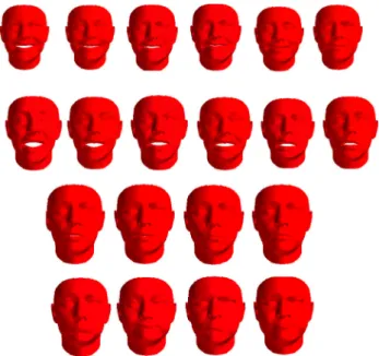
Moreover, to be able to develop the categorical emotion synthesis model, we used the 2000 expressive 3D meshes per basic expression (12,000 meshes in total) that were pro-vided along with 4DFAB. Those 3D meshes corresponded to (annotated) apex frames of posed expression sequences in 4DFAB. Such examples are shown in Fig.1.

3.2 4DFAB Dimensional Annotation

Targeting to develop the novel dimensional expression synthesis method, all 1580 dynamic 3D sequences (i.e., over 600,000 frames) of 4DFAB have been annotated in terms of valence and arousal emotion dimensions. In total, three experts were chosen to perform the annotation task. Each expert performed a time-continuous annotation for

AN DI FE J SA SU

Fig. 1 Examples from the 4DFAB of apex frames with posed expres-sions for the six basic expresexpres-sions: Anger (AN), Disgust (DI), Fear (FE), Joy (J), Sadness (SA), Surprise (SU)

both affective dimensions. The application-tool described in Zafeiriou et al. (2017), was used in the annotation process.

Each expert logged into the application-annotation tool using an identifier (e.g. his/her name) and selected an appro-priate joystick; then the application showed a scrolling list of all videos and the expert selected a video to annotate; then a screen appeared that showed the selected video and a slider of valence or arousal values ranging in[−1,1]; the expert annotated the video by moving the joystick either up or down; finally, a file was created with the annotations. The mean inter-annotation correlation per annotator was 0.66, 0.70, 0.68 for valence and 0.59, 0.62, 0.59 for arousal. The average of those mean inter-annotation correlations was 0.68 for valence and 0.60 for arousal. Those values are high, indicating a very good agreement between annotators. As a consequence, the final label values were chosen to be the mean of those three annotations.

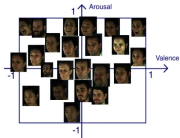
Examples of frames from the 4DFAB along with their annotations, are shown in Fig.2. Figure3shows the 2D his-togram of annotations of 4DFAB. In the rest of the paper, we refer to the 4DFAB database either as: (i) the 600,000 frames with their corresponding 3D meshes, which have been anno-tated with 2D valence and arousal (VA) emotion values or (ii) the 12,000 apex frames of posed expressions with their cor-responding 3D meshes, which have categorical annotation.

3.3 Mesh Pre-Processing: Establishing Dense

Correspondence

Each 3D mesh is first re-parameterized into a consistent form where the number of vertices, the triangulation and the anatomical meaning of each vertex are made consistent

Fig. 2 The 2D valence-arousal space and some representative frames of 4DFAB

Fig. 3 The 2D histogram of annotations of 4DFAB

across all meshes. For example, if the vertex with index i in one mesh corresponds to the nose tip, it is required that the vertex with the same index in every mesh corresponds to the nose tip too. Meshes satisfying the above properties are said to be in dense correspondence with one another. So, correlat-ing all these meshes with a universal coordinate frame (viz. a 3D face template) is a step to follow so as to establish dense correspondence.

In order to do so, we need to define a 2DUVspace for each mesh, which in fact is a contiguous flattened atlas that embeds the 3D facial surface. Such a UV space is associated with its corresponding 3D surface through a bijective mapping; thus, establishing dense correspondence between two UV images implicitly establishes a 3D-to-3D correspondence for the mapped mesh. UV mapping is the 3D modelling process of projecting a 2D image to a 3D model’s surface for texture mapping. The letters U andV denote the axes of the 2D

texture, sinceX, YandZare already taken to denote the axes of the 3D object in model space.

We employ an optimal cylindrical projection method (Booth and Zafeiriou 2014) to synthetically create a UV space for each mesh. A UV map (which is an image I), with each pixel encoding both spatial information (X, Y, Z) and texture information (R, G, B), is produced, on which we perform non-rigid alignment. Non-rigid align-ment is performed through the UV-TPS method that utilises key landmarks fitting and Thin Plate Spline (TPS) warp-ing (Cosker et al. 2011). Following Cheng et al. (2018), we perform several modifications to Cosker et al. (2011), to suit our data. Firstly, we build session-and-person-specific Active Appearance Models (AAMs) (Alabort-i Medina and Zafeiriou 2017) to automatically track feature points in the UV sequences. This means that 4 different AAMs are built and used separately for one subject. Main reasons behind this are:(i) textures of different sessions differ due to several facts (i.e. aging, beards, make-ups, experiment lighting condition), (ii) person-specific model is proven more accurate and robust in specific domains (Chew et al.

2012).

In total, 435 neutral meshes and 1047 expression meshes (1 neutral and 2–3 expressive meshes per person and session) in 4DFAB were selected; these contained annotations with 79 3D landmarks. They were unwrapped and rasterised to UV space, then grouped for building the corresponding AAMs. Each UV map was flipped to increase fitting robustness. Once all the UV sequences were tracked with 79 landmarks, they were then warped to the corresponding reference frame using TPS, thus achieving the 3D dense correspondence. For each subject and session, one specific reference coor-dinate frame from his/her neutral UV map was built. From each warped frame, we could uniformly sample the texture and 3D coordinates. Eventually, a set of non-rigidly corre-sponded 3D meshes under the same topology and density were obtained.

Given that meshes have been aligned to their designated reference frame, the last step was to establish dense 3D-to-3D correspondences between those reference frames and a 3D template face. This is a 3D mesh registration problem, solved by Non-rigid ICP (Amberg et al.2007). We employed it to register the neutral reference meshes to a common tem-plate, the Large Scale Facial Model (LSFM) (Booth et al.

2018). We brought all 600,000 3D meshes into full corre-spondence with the mean face of LSFM. As a result, we created a new set of 600,000 3D faces that share identi-cal mesh topology, while maintaining their original facial expressions. In the following, this set constitutes the 3D facial expression gallery which we use for facial affect syn-thesis.

3.4 Constructing a 3D Morphable Model

A common 3DMM consists of three parametric models: the shape, the camera and the texture models.

To build the shape model, the training 3D meshes should be put in dense correspondence (similarly to the previ-ous Mesh Pre-Processing subsection). Next, Generalized Procrustes Analysis is performed to remove any similarity effects, leaving only shape information. Finally, Principal Component Analysis (PCA) is applied to these meshes, which generates a 3D deformable model as a linear basis of shapes. This model allows for the generation of novel shape instances. The model can be expressed as:

S(p)= ¯s+Usp (1)

where¯s∈ R3Nis the mean component of 3D shape (in our case it is the mean of shape models from the LSFM model described in the next subsection) withN denoting the num-ber of vertices in the shape model;Us ∈R3N×ns is the shape eigenbase (in our case it is the identity subspace of LSFM) withns <<3N being the number of principal components (ns is chosen to explain a percentage of the training set vari-ance; generally, this percentage is 99.5%); andp∈Rns is a vector of parameters which allows for the generation of novel shape instances.

The purpose of camera model is to project the object-centered Cartesian coordinates of a 3D mesh instance into 2D Cartesian coordinates in an image plane. At first, given that the camera is static, the 3D mesh is rotated and trans-lated using a linear view transformation, which results in 3D rotation and translation components. Then, a nonlinear perspective transformation is applied. Note that quaternions (Kuipers et al 1999; Wheeler and Ikeuchi 1995) are used to parametrise the 3D rotation, which ensures computa-tional efficiency, robustness and simpler differentiation. In this manner we construct the camera parameters (i.e., 3D translation components, quaternions and parameter of lin-ear perspective transformation). The camera model of the 3DMM applies the above transformations on the 3D shape instances generated by the shape model. Finally, the camera model can be written as:

W(p,c)=P(S(p),c), (2)

where S(p)is a 3D face instance;c∈ Rnc are the camera parameters (for rotation, translation and focal length;ncis 7); andP:R3N →R2N is the perspective camera projection.

For the texture model, large facial “in-the-wild” data-bases annotated for sparse landmarks are needed. Let us assume that the meshes have corresponding camera and

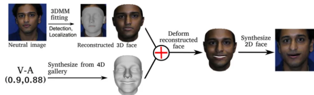
Fig. 4 The facial affect synthesis framework: the user inputs an arbitrary 2D neutral face and the affect to be synthesized (a pair of valence-arousal values in this case)

shape parameters. These images are passed through a dense feature extraction function that returns feature-based rep-resentations for each image. These are then sampled from the camera model at each vertex location so as to build a texture sample, which will be nonsensical for some regions mainly due to self occlusions present in the mesh projected in the image space. To complete the missing information of the texture samples, Robust PCA (RPCA) with missing val-ues (Shang et al.2014) is applied. This produces complete feature-based textures that can be processed with PCA to cre-ate the statistical model of texture, which can be written as:

T(λ)=t+Utλ, (3)

wheret ∈R3N is the mean texture component (in our case it is the mean of texture model from LSFM);Ut ∈ R3N×nt andλ∈Rnt are the texture subspace (eigenbase) and texture parameters, respectively, withnt <<3N being the number of principal components. This model can be used to generate novel 3D feature-based texture instances.

3.4.2 The Large Scale Facial Model (LSFM)

We have adopted the LSFM model constructed using the MeIn3D dataset (Booth et al. 2018). The construction pipeline of LSFM starts with a robust approach to 3D land-mark localization resulting in generating 3D landland-marks for the meshes. The 3D landmarks are then employed as soft constraints in Non-rigid ICP to place all meshes in corre-spondence with a template facial surface; the mean face of the Basel Face Model (Paysan et al.2009) has been chosen. However, the large cohort of data could result in convergence failures. These are an unavoidable byproduct of the fact that both landmark localization and NICP are non-convex opti-mization problems sensitive to initialization.

A refinement post-processing step weeds out problematic subjects automatically, guaranteeing that the LSFM models are only constructed from training data for which there exist a high confidence of successful processing. Finally, the LSFM models are derived by applying PCA on the corresponding training sets, after excluding the shape vectors that have been classified as outliers. In total, 9663 subjects are used to build LSFM, which covers a wide variety of age (from 5 to over

80s), gender (48% male, 52% female), and ethnicity (82% White, 9% Asian, 5% Mixed Heritage, 3% Black and 1% other).

4 The Proposed Approach

In this section, we present the fully automatic facial affect synthesis framework. The user needs to provide a neutral image and an affect, which can be a VA pair of values, a path in the 2D VA space, or one of the basic expression categories. Our approach: (1) performs face detection and landmark localization on the input neutral image, (2) fits a 3D Morphable Model (3DMM) on the resulting image (Booth et al.2017), (3) deforms the reconstructed face and adds the input affect, and (4) blends the new face with the given affect into the original image. Here let us note that the total time needed for the first two steps is about 400ms; this has to be performed only once, if generating multiple images from the same input image. Specific details regarding the described steps of our approach follow. This procedure is shown in Fig.4.

4.1 Face Detection and Landmark Localization

The first step to edit an image is to locate landmark points that will be used for fitting the 3DMM. We first perform face detection with the face detection model from Zhang et al. (2016) and then utilize (Deng et al.2018) to localize 68 2D facial landmark points which are aware of the 3D structure of the face, in the sense that points on occluded parts of the face (most commonly part of the jawline) are correctly localized.

4.2 3DMM-Fitting: Cost Function and Optimization

The goal of this step is to retrieve a reconstructed 3D face with the texture sampled from the original image. In order to do so, we first need a 3DMM; we select the LSFM.

Fitting a 3DMM on face images is an inverse graphics approach to 3D reconstruction and consists of optimizing three parametric models of the 3DMM, the shape,texture andcameramodels. The optimization aims at rendering a 2D

image which is as close as as possible to the input one. In our pipeline we follow the 3DMM fitting approach of Booth et al. (2017). As is already noted, we employ the LSFM (Booth et al.2018)S(p)to model the identity deformation of faces. Moreover, we adopt the robust, feature-based texture model T(λ)of Booth et al. (2017), built from in-the-wild images. The employed camera model is a perspective transformation W(p,c), which projects shapeS(p)on the image plane.

Consequently, the objective function that we optimize can be formulated as: argminp,λ,cF(W(p,c))−T(λ)2+clWl(p,c)−sl2 + csp2−1 s +ctλ 2 −1 t , (4)

where the first term denotes the pixel loss between the fea-ture based imageFsampled at the projected shape’s locations and the model generated texture; the second term denotes a sparse landmark loss between the image 2D landmarks and the corresponding 2D projected 3D points, where the 2D shape,sl, is provided by Deng et al. (2018); the rest two terms are regularization terms which serve as counter over-fitting mechanism, where 6s and6t are diagonal matrices with the main diagonal being eigenvalues of the shape and texture models respectively;cl,csandctare weights used to regularize the importance of each term during optimization and were empirically set to 105, 3×106and 1, respectively, following Booth et al. (2017). Note also, that the 2D land-marks term is useful as it drives the optimization to converge faster. Problem of Eq.4is solved by the Project-Out variation of Gauss-Newton optimization as formulated in Booth et al. (2017).

From the optimized models, the optimal shape instance constitutes the neutral 3D representation of the input face. Moreover, by utilizing the optimal shape and camera mod-els, we are able to sample the input image at the projected locations of the recovered mesh and extract a UV texture, that we later use for rendering.

4.3 Deforming Face and Adding Affect

Given an affect and an arbitrary 2D imageI, we first fit the LSFM to this image using the aforementioned 3DMM fitting method. After that, we can retrieve a reconstructed 3D face

sor igwith the texture sampled from the original image

(tex-ture sampling is simply extracting image pixel value for each projected 3D vertex in image plane). Let us assume that we have created an affect synthesis modelMA f f that takes the affect as input and generates a new expressive face (denoted as sgen), i.e., s = MA f f(a f f ect)(specific details regard-ing the generation of the expressive face, can be found in Sect.4.5). Next, we calculate the facial deformationsby subtracting the synthesized facesgen from the LSFM

tem-plates¯, i.e.,s=sgen− ¯s, and impose this deformation on the reconstructed mesh, i.e.,snew =sor ig+s. Therefore, we obtain a 3D face (dubbedsnew) with facial affect.

4.4 Synthesizing 2D Face

The final step in our pipeline is to render the new 3D face

snewback to the original 2D image. To do that we employ the mesh that we have deformed according to the given affect, the extracted UV texture and the optimal camera transforma-tion of the 3DMM. For rendering, we pass the three model instances to a renderer and we use as background the back-ground of the input image. Lastly, the rendered image is fused with the original image via poisson blending (Pérez et al.2003) to smooth the boundary between foreground face and image background so as to produce a natural and real-istic result. In our experiments, we used both a CPU-based renderer (Alabort-i-Medina et al. 2014) and a GPU-based renderer (Genova et al. 2018). The GPU-based renderer greatly decreases the rendering time, as it needs 20 ms to render a single image, while the CPU-based renderer needs 400 ms.

4.5 Synthesizing Expressive Faces with Given Affect

Models and Computing Mean Faces

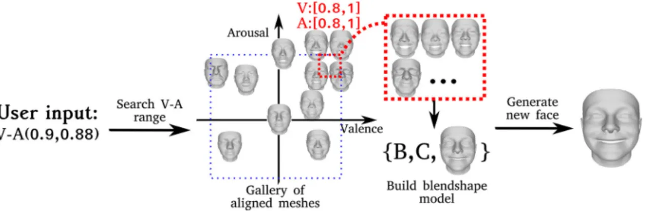
Let us first describe the VA case. We have 600,000 3D meshes (established into dense correspondence) and their VA anno-tations. We want to appropriately discretize the VA space into classes, so that each class contains a sufficient number of data. This is due to the fact that if classes contain only few examples, it is more likely to include identity information. However, the synthesized facial affect should only describe the expression associated with the VA pair of values, rather than information for the person’s identity, gender, or age. We have chosen to perform agglomerative clustering (Maimon and Rokach 2005) on the VA values, using the euclidean distance as metric and the ward as linkage criterion (keep-ing the correspondence between VA values and 3D meshes). In this manner, we created 550 clusters, i.e., classes. Then we built blendshape models and computed the mean face per class. Figure5illustrates the mean faces of various classes. It should be mentioned that the majority of classes correspond to the first two quadrants of the VA space, namely the regions of positive valence (as can be seen in the 2D histogram of Fig.3).

As far as the basic expression case is concerned, based on the derived 12,000 3D meshes, 2000 for each of the six basic expressions, we built six blendshape models and six corresponding mean faces.

Fig. 5 Some mean faces of the 550 classes in the VA space

4.5.2 User Selection: VA/Basic Expr and Static/Temporal Synthesis

The user first chooses the type of affect that our approach will generate. The affect could be either a point, or a path in the VA space, or one the six basic expression categories. If the user chooses the latter, then we retrieve the mean face of this category and add it on the 3D face reconstructed from the user’s input neutral image. In this case, the only difference in Fig.4would be for the user to input a basic expression, the happy one, instead of a VA pair of values. If the user chooses the former, then (s)he needs to additionally clarify if our approach should generate an image (‘static synthe-sis’) or a sequence of images (‘temporal synthesynthe-sis’) with this affect.

Static synthesis If the user selects ‘static synthesis’, then the user should input a specific VA pair of values. Then, we retrieve the mean face of the class to which this VA value belongs. We use this mean face as the affect to be added on the 3D face reconstructed from the provided neutral image. Figure4shows the proposed approach for this specific case. Figure6 illustrates the procedure described in Sect. 4.5.1

given that the 550 VA classes are already created.

Temporal synthesisIf the user selects ‘temporal synthesis’, then, (s)he should provide a path in the VA space (for instance by drawing) that the synthesized sequence should follow. Then, we retrieve the mean faces of the classes to which the VA values of the path belong. We use each of these mean faces as the affect to be added on the 3D faces reconstructed from the provided neutral image. As a consequence, an expressive

sequence is generated that shows the evolution of affect on the VA path specified by the user.

Here let us mention that the fact that the 4DFAB used in our approach is a temporal database, ensures that suc-cessive video frames’ annotations are adjacent in the VA space, since they generally show the same or slightly dif-ferent states of affect. Thus, the 3D meshes of successive video frames will lie in the same and in adjacent classes in the 2-D VA space. Thus mean faces from adjacent classes can be used to show temporal evolution of affect as was above described.

4.5.3 Expression Blendshape Models

Expression blendshape models provide an effective way to parameterize facial behaviors. The localized blendshape model (Neumann et al. 2013) has been used to describe the selected VA samples. To build this model, we first bring all meshes into full correspondence following the dense registration approach described in Sect. 3.3. As a result, we have a set of training meshes with the same number of vertices and identical topology. Note that we have also selected one neutral mesh for each subject, which should have full correspondence with the rest data. Next, we subtract each 3D mesh from the respective neutral mesh, and create a set of m difference vectors

di ∈ R3N. We then stack them into a matrix D = [d1, . . . ,dm] ∈ R3N×m, where N is number of ver-tices in the mesh. Finally, a variant of sparse Princi-pal Component Analysis (PCA) is applied to the data matrixD, so as to identify sparse deformation components

C∈Rh×1:

arg minD−BC2_F+ (C) s.t.V(B) , (5) where the constraint V can be either max(|Bk|) = 1, ∀k or max(Bk) = 1, B ≥ 1, ∀k, with Bk ∈ R3N×1 denoting thekth components of sparse weight matrixB =

[B1, . . . ,Bh]. Selection of these two constraints depends on the actual usage; the major difference is that the lat-ter one allows for negative weights and therefore enables deformation towards both directions, which is useful for describing shapes like muscle bulges. In this paper, we have selected the latter constraint, as we wish to enable bidirec-tional muscle movement and synthesise a rich variety of expressions. The regularization of sparse componentsCwas performed with1/2 norm (Wright et al.2009; Bach et al.

2012). To permit more local deformations, additional reg-ularization parameters were added into (C). To compute optimalCandB, an iterative alternating optimization was employed (please refer to Neumann et al. 2013 for more details).

Fig. 6 Generation of new facial affect from the 4D face gallery; the user provides a target VA pair

5 Databases

To evaluate our facial affect synthesis method in different sce-narios (e.g. controlled laboratory environment, uncontrolled in-the-wild setting), we utilized neutral facial images from as many as 15 databases (both small and large in terms of size). Table1briefly presents the Multi-PIE (Gross et al.2010), Aff-Wild (Kollias et al.2019; Zafeiriou et al.2017), AFEW 5.0 (Dhall et al.2017), AFEW-VA (Kossaifi et al.2017), BU-3DFE (Yin et al.2006), RECOLA (Ringeval et al.2013), AffectNet (Mollahosseini et al.2017), RAF-DB (Li et al.

2017), KF-ITW (Booth et al.2017), Face place, FEI (Thomaz and Giraldi2010), 2D Face Sets and Bosphorus (Savran et al.

2008) databases that we used in our experimental study. Let us note that for AffectNet no test set is released and thus we use the released validation set to test on and randomly divide the training set into a training and a validation subset (with a 85/15 split).

Table 1 presents these databases by showing:(i) the model of affect they use, their condition, their type (static images or audiovisual image sequences), the total num-ber of frames and (male/female) subjects that they contain and the range of ages of the subjects, and (ii) the total number of images that we synthesized using our approach (both in the valence-arousal and the six basic expressions cases).

6 Experimental Study

This section describes the experiments performed so as to evaluate the proposed approach. At first, we provide a qualitative evaluation of our approach by showing many synthesized images or image sequences from all fifteen databases described in the previous Section; as well as

by comparing images generated by state-of-the-art GANs (StarGAN, GANimation) and our approach. Next, a quan-titative evaluation is performed by using the synthesized images as additional data to train Deep Neural Networks (DNNs); it is shown that the trained DNNs outperform cur-rent state-of-the-art networks and GAN-based methods on each database. Finally an ablation study is performed in which:(i) the synthesized data are considered and used as a training (test) dataset, while the original data are respec-tively used as test (training) dataset, (ii) the effect of the amount of synthesized data on network performance is studied, (iii) an analysis is performed based on subjects’ age.

6.1 Qualitative Evaluation of Achieved Facial Affect

Synthesis

We used all databases mentioned in Sect. 5 to supply the proposed approach with ‘input’ neutral faces. We then synthesized the emotional state corresponding to specific affects (both in VA case and in the six basic expressions one) for these images. At first we show many generated images (static synthesis) according to different VA values, then we illustrate examples of generated image sequences (temporal synthesis) and next we present some synthe-sized (static) images according to the six basic expressions. Finally, we visually compare images generated by our approach with synthesized images by StarGAN and GANi-mation.

6.1.1 Results on Static and Temporal Affect Synthesis Figure7shows representative results of facial affect synthe-sis, when user inputs a VA pair and selects to generate a static image. These results are organized in three age groups:

Table 1 Databases u sed in our approach, along with their p roperties and the number o f synthesized images in the v alence-arousal case and the six basic express ions one; ‘static’ m eans images, ‘A /V’ m eans audio v isual sequences, i.e., videos Databases (DBs) DB type Model o f af fect Condition DB size # o f subjects A ge range T o tal # of synthesized images V A Basic E xpr MUL T I-PIE (Gross et al. 2010 ) Static Neutral, Surprise, D isgust, Smile + S quint, S cream Controlled 755,370 337 Male: 235 Female: 102 – 52,254 5520 Kinect fusion ITW (Booth et al. 2017 ) Static Neutral, Happiness , Surprise In-the-wild 3264 17 – 116,235 12,236 FEI (Thomaz and G iraldi 2010 ) Static Neutral, Smile C ontrolled 2800 200 Male: 100 Female: 100 19–40 11,400 1200 F ace place a Static 6 B asic Expr , N eutral, Confusion Controlled 6574 235 Male: 143 Female: 9 2 – 59,736 6288 AFEW 5.0 (Dhall et al. 2017 ) A/V 6 Basic E xpr , N eutral In-the-wild 41,406 > 330 1–77 705,649 56,514 RECOLA (Ringe v al et al. 2013 ) A/V V A C ontrolled 345,000 46 Male: 1 9 Female: 2 7 – 46,455 4890 BU -3 D F E (Y in et al . 2006 ) S tatic 6 Basic E xpr , N eutral Controlled 2500 100 Male: 5 6 Female: 4 4 18–70 5700 600 Bosphorus (Sa v ran et al. 2008 ) Static 6 B asic Expr Controlled 4666 105 Male: 6 0 Female: 4 5 25–35 17,018 1792 Af fectNet (Mollahosseini et al. 2017 ) Static V A + 6 Basic E xpr , N eutral + C ontempt In-the-wild 450,000 manually annotated –0 to > 50 2,476,235 176,425 Af f-wild (K o llias et al. 2019 ; Z afeiriou et al. 2017 ) A/V V A In-the-wild 1,224,094 200 Male: 130 Female: 7 0 – 60,135 6330 AFEW -V A (K o ssaifi et al. 2017 ) A/V V A In-the-wild 30,050 < 600 – 108,864 11,460 R A F -D B (L ie ta l. 2017 ) S tatic 6 Basic, Neutral + 11 Compound Expr In-the-wild 15,339 + 3954 – 0–70 121,866 12,828 2D face sets b: P ain S tatic 6 B asic, N eutral + 1 0 P ain Expr Controlled 599 23 Male: 1 3 Female: 1 0 – 2736 288 2D face sets: Iranian Static Neutral, Smile Controlled 369 34 Male: 0 Female: 3 4 – 2679 282 2D face sets: N ottingham scans Static Neutral C ontrolled 100 100 Male: 5 0 Female: 5 0 – 5700 600 aStimulus images courtesy of Michael J. T arr , C enter for the N eural B asis of Cognition and Department of Psychology , C arne gie M ellon U ni v ersity , http:// www .tarrlab .or g / bhttp:// p ics.stir .ac.uk

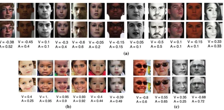
Fig. 7 VA Case of static (facial) synthesis across all databases; first rows show the neutral, second ones show the corresponding synthesized images and third rows show the corresponding VA values. Images of:bkids,celderly people andain-between ages, are shown

Fig.7b kids, Fig.7c elderly people and Fig.7a in-between ages. In each part, the first row illustrates neutral images sam-pled from each of the aforementioned databases, the second one shows the respective synthesized images and the third shows the respective VA values that were synthesized. More-over, Fig.8shows neutral images on the left hand side (first column) and synthesized images, with various valence and arousal values, on the right hand side (following columns). It can be observed that the synthesized images are identity preserving, realistic and vivid. Figure9 refers to the basic expression case; it shows neutral images on the left hand side of (a) and (b) and synthesized images with basic expressions on the right hand side. Figure10illustrates the VA case for temporal synthesis, as was described in Sect.4.5.2. Neutral images are shown on the left hand side, while synthesized face sequences with time-varying levels of affect are shown on the right hand side.

All these figures show that the proposed framework works well, when using images from either in-the-wild, or con-trolled databases. This indicates that we can effectively synthesize facial affect irregardless of image conditions (e.g., occlusions, illumination and head poses).

6.1.2 Comparison with GANs

In order to characterize the value that the proposed approach imparts, we provide qualitative comparisons with two state-of-the-art GANs, namely StarGAN (Choi et al.2018) and GANimation. Like CycleGAN (referenced in Sect.2), Star-GAN performs image-to-image translation, but adopts a

unified approach such that a single generator is trained to map an input image to one of multiple target domains, selected by the user. By sharing the generator weights among different domains, a dramatic reduction of the number of parameters is achieved. GANimation was described in Sect.2.

At first, it should be mentioned that, the original StarGAN synthesized images according to the basic expressions (apart from facial attributes) and the GANimation synthesized images according to AUs. However, in psychology, there does not exist any mapping between AUs–VA and no con-sistent mapping (across studies) between AUs-expressions, or VA-expressions. In order to achieve a fair comparison of our method with these networks, we applied them—for the first time—to the VA space; we trained them with the same 600,000 frames of 4DFAB that we used in our approach. In both networks, pre-processing was conducted, which included face detection and alignment. For a fair comparison, in all presented results (both qualitative and quantitative), the GANs were provided with the same neutral images and the same VA values.

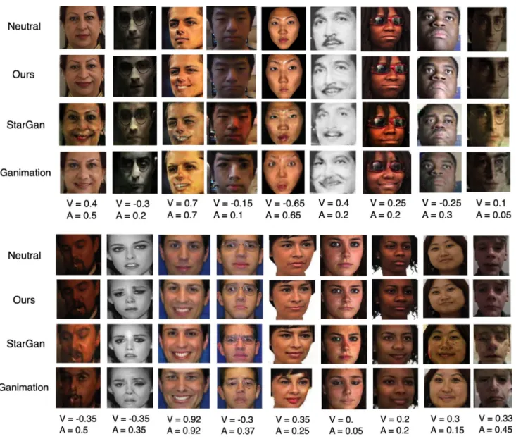
Figure11presents a visual comparison between images generated by our approach, StarGAN and GANimation. It shows the neutral images, the synthesized VA values and the resulting images. It is evident that our approach synthe-sizes samples that:(i) look much more natural and realistic, (ii) maintain the degree of sharpness of the original neutral image, and (iii) combine visual accuracy with spatial resolu-tion.

Some further deductions can be made from Fig. 11. StarGAN does not perform well when tested on different

in-Fig. 8 VA case of facial synthesis: on the left hand side are the neutral 2D images and on the right the synthesized images with different levels of affect

Fig. 9 Basic Expression Case of facial synthesis: on the left hand side ofaandbare the neutral 2D images and on the right the synthesized images with some basic expressions

the-wild and controlled databases that include variations in illumination conditions and head poses. StarGAN is unable to reflect detailed illumination; unnatural lighting changes were observed on the results. These can be explained because in the original StartGAN paper (Choi et al.2018), its capability

to generate affect has not been tested on in-the-wild facial analysis (we refer only to the case of emotion recognition). In general, StarGAN yields more realistic results when it is trained simultaneously with multiple datasets annotated for different tasks.

Additionally, in Choi et al. (2018), when referring to emotion recognition, StarGAN was trained and evaluated on Radboud Faces Database (RaFD) (Langner et al. 2010) which:(i) is very small in terms of size (around 4800 images) and (ii) is a lab-controlled and posed expression database. Last but not least, StarGAN has been tested to change only a particular aspect of a face among a discrete number of attributes/emotions defined by the annotation granularity of the dataset. As can be seen in Fig. 11, StarGAN cannot accurately provide realistic results when tested in the much broader and more difficult task of valence and arousal gen-eration (and estimation).

As far as GANimation is concerned, its results are also worse than the results of our approach. In most cases, it shows artifacts and in some cases certain levels of blur-riness. When compared to StarGAN, GANimation seems more robust to changing backgrounds and lighting condi-tions; this is due to the attention and color masks that it contains. Nevertheless, in general, errors in the attention mechanism occur when the input contains extreme expres-sions. The attention mechanism does not seem to sufficiently weight the color transformation, causing transparencies. It is interesting to note that on the Leonardo DiCaprio image, the synthesized image by GANimation shows open eyes, whereas on the neutral image (and the one synthesized by our approach) eyes are closed; this illustrates errors of the mask. For example, in Fig.11, images produced by GAN-imation in columns 1, 3, 4, 5, 6, 9 show the discussed problems.

6.2 Quantitative Evaluation of the Facial Affect

Synthesis Through Data Augmentation

It is generally accepted that using more training data—of good quality—leads to better results in supervised train-ing. Data augmentation increases the effective size of the training dataset. In this section we present a data augmenta-tion strategy which uses the synthesized data produced by our approach, as additional data to train DNNs, for both valence-arousal prediction, as well as classification into the basic expression categories. In particular, we describe exper-iments performed on eight databases, presenting the adopted evaluation criteria, the networks we used and the obtained results. We also report the performances of the networks trained—in a data augmentation manner—with synthesized images from StarGAN and GANimation. It is shown that the DNNs trained with the proposed data augmentation method-ology outperform both the state-of-the-art techniques and the

Fig. 10 VA case of temporal (facial) synthesis: on the left hand side are the neutral 2D images and on the right the synthesized image sequences

DNNs trained with StarGAN and GANimation, in all exper-iments, validating the effectiveness of the proposed facial synthesis approach. Let us first explain some notations. In the followings, by reporting ‘network_name trained using StarGAN’, ‘network_name trained using GANimation’ and ‘network_name trained using the proposed approach’, we refer to networks trained with the specific database’s training set augmented with data synthesized by StarGAN, GANima-tion and the proposed approach, respectively.

6.2.1 Leveraging Synthesized Data for Training Deep Neural Networks: Valence-Arousal Case

In this set of experiments we consider four facial affect databases annotated in terms of valence and arousal, the Aff-Wild, RECOLA, AffectNet and AFEW-VA data-bases. At first, we selected neutral frames from these databases, i.e., frames with zero valence and arousal values (human inspec-tion was also conducted to make sure that they represented

neutral faces). For every frame, we synthesized facial affect according to the methodology described in Sect.4. We start by first describing the evaluation criteria used in our experi-ments.

6.2.2 The Adopted Evaluation Criteria

The main evaluation criterion that we use is the Concordance Correlation Coefficient (CCC) (Lawrence, and Lin 1989), which has been widely used in related Challenges (e.g., Val-star et al. 2016); we also report the Mean Squared Error (MSE), since this has been also frequently used in related research.

CCC evaluates the agreement between two time series by scaling their correlation coefficient with their mean square difference. CCC takes values in the range[−1,1], where+1 indicates perfect concordance and −1 denotes perfect dis-cordance. Therefore high values are desired. CCC is defined as follows:

Fig. 11 Generated results by our approach, StarGAN and GANimation ρc= 2sx y s2 x+s2y+(x¯− ¯y)2 , (6)

wheresx andsy are the variances of the ground truth and predicted values respectively,x¯andy¯are the corresponding mean values andsx yis the respective covariance value.

The Mean Squared Error (MSE) provides a simple com-parative metric, with a small value being desirable. MSE is defined as follows: M S E= 1 N N i₌1 (xi−yi)2, (7)

where x and y are the ground truth and predicted values respectively andN is the total number of samples.

In some cases we also report the Pearson-CC (P-CC) and the Sign Agreement Metric (SAGR), since they have been reported by respective state-of-the-art methods.

The P-CC takes values in the range[−1,1]and high values are desired. It is defined as follows:

ρx y = sx y sxsy,

(8)

wheresxandsyare the variances of the ground truth and pre-dicted values respectively andsx yis the respective covariance value.

The SAGR takes values in the range [0,1], with high values being desirable. It is defined as follows:

S AG R= 1 N N = δ(sign(xi),sign(yi)), (9)

Table 2 Aff-Wild: CCC and MSE evaluation of valence and arousal predictions provided by the VGG-FACE-GRU trained using our approach versus state-of-the-art networks and methods

Networks CCC MSE

Valence Arousal Valence Arousal FATAUVA-Net (Chang et al.2017) 0.396 0.282 0.123 0.095 VGG-FACE-GRU trained using StarGAN 0.556 0.424 0.085 0.060 VGG-FACE-GRU trained using GANimation 0.576 0.433 0.077 0.057 AffWildNet (Kollias et al.2017,2019) 0.570 0.430 0.080 0.060 VGG-FACE-GRU trained using the proposed approach 0.595 0.445 0.074 0.051

Valence and arousal values are in[−1,1]

Bold values correspond to the results of the best methods

where N is the total number of samples, x and y are the ground truth and predicted values respectively,δis the Kro-necker delta function andδ(sign(x),sign(y))is defined as:

δ(sign(x),sign(y))= ⎧ ⎪ ⎨ ⎪ ⎩ 1, x0 and y0 1, x0 and y0 0, otherwise (10)

6.2.3 Experiments on Dimensional Affect

Aff-WildWe synthesized 60,135 images from the Aff-Wild database and added those images to the training set of the first Affect-in-the-wild Challenge. The employed network archi-tecture was the AffWildNet (VGG-FACE-GRU) described in Kollias et al. (2017,2019).

Table 2 shows a comparison of the performance of: the VGG-FACE-GRU trained using: (i) our approach, (ii) StarGAN, and (iii) GANimation; the best performing net-work, AffWildNet, reported in Kollias et al. (2017, 2019); the winner of the Aff-Wild Challenge (Chang et al.2017) (FATAUVA-Net).

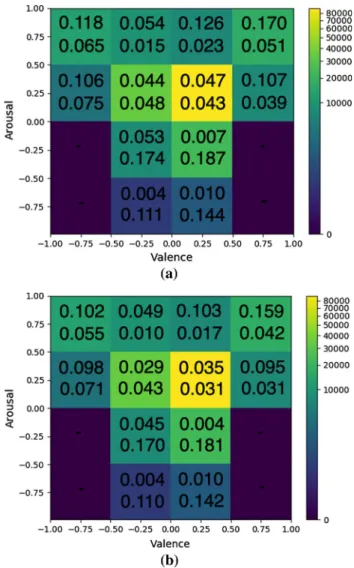
From Table2, it can be verified that the network trained on the augmented dataset, with synthesized by our approach images, outperformed all other networks. It should be noted that the number of synthesized images (around 60K) was small compared to the size of Aff-Wild’s training set (around 1M), the latter being already sufficient for training the best performing DNN; consequently, the improvement was not large, about 2%. An interesting observation is that the net-work trained using StarGAN displayed worse performance than AffWildNet. This means that the 68 landmark points that were passed as additional input to the AffWildNet helped the network in reaching a better performance than just adding a small amount (compared to the training set size) of auxiliary synthesized data. The MSE error improvement on Valence and Arousal estimation provided by the augmented training versus the AffWildNet one, over the different areas of the VA space, is shown through the 2D histograms presented in Fig.12. It can be seen that the improvement on MSE was

Fig. 12 The 2D histogram of valence and arousal Aff-Wild’s test set annotations, along with the MSE per grid area, in the case ofa AffWild-Net andbVGG-FACE-GRU trained using the proposed approach

better in areas in which a larger number of new samples was generated, i.e., in the positive valence regions.

RECOLAWe generated 46,455 images from RECOLA; this number corresponds to around 40% of its training data set size. The employed network architecture was the ResNet-GRU described in Kollias et al. (2019).

Table 3 RECOLA: CCC evaluation of valence and arousal predictions provided by the ResNet-GRU trained using the proposed approach versus other state-of-the-art networks and methods

Networks CCC

Valence Arousal

ResNet-GRU (Kollias et al.2019) 0.462 0.209

ResNet-GRU trained using StarGAN 0.503 0.245

ResNet-GRU trained using GANimation 0.486 0.222

Fine-tuned AffWildNet (Kollias et al.2019) 0.526 0.273 ResNet-GRU trained using the proposed approach 0.554 0.312

Bold values correspond to the results of the best methods

Table3 shows a comparison of the performance of: the ResNet-GRU network trained using:(i) our approach, (ii) StarGAN, and (iii) GANimation; the AffWildNet fine-tuned on the RECOLA, as reported in Kollias et al. (2019); a ResNet-GRU directly trained on RECOLA, as reported in Kollias et al. (2019).

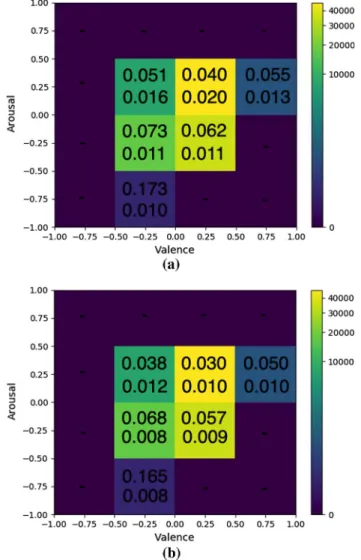
From Table3, it can be verified that the network trained using the proposed approach outperformed all other net-works. The above gains in performance can be justified by the fact that the number of synthesized images (around 46,500) was significant compared to the size of RECOLA’s training set (around 120,000) and that the original training set size was not very sufficient to train the DNNs. It is worth mentioning that the GAN based methods have not managed to provide a sufficiently enriched dataset so that a similar boost in the achieved performances could be obtained. The MSE error improvement on Valence and Arousal estimation provided by the augmented training versus the original one (which was 0.045–0.100 versus. 0.055–0.160), over the different areas of the VA space, is shown through the 2D histograms presented in Fig.13. Big reduction of MSE value was achieved in all covered VA areas.

AffectNetThe AffectNet database contains around 450,000 manually annotated images and around 550,000 automati-cally annotated images for valence-arousal. We only used the manually annotated images so as to be consistent with the state-of-the-art networks that were also trained using this set. Additionally, the manually annotated set ensures that the images used by our approach to synthesize new, are indeed neutral. We created 2,476,235 synthesized images from the AffectNet database, a number that is more than 5 times bigger than the training data size. The employed network architec-ture was VGG-FACE. For comparison purposes, we trained the network using the original training data set (let us call this network ‘the VGG-FACE baseline’).

Table4 shows a comparison of the performance of: the VGG-FACE baseline; the VGG-FACE trained using:(i) our approach, (ii) StarGAN, and (iii) GANimation; AlexNet, which is the baseline network of the AffectNet database (Mollahosseini et al.2017).

From Table4, it can be verified that the network trained by the proposed methodology outperformed all other networks.

Fig. 13 The 2D histogram of valence and arousal RECOLA’s test set annotations, along with the MSE per grid area, in the case ofa ResNet-GRU andbResNet-GRU trained using the proposed approach

This boost in performance has been large, in all evaluation criteria, compared to the VGG-FACE baseline network, with spread of this improvement over the VA space shown in Fig. 14. The explanation arises from the large number of synthesized images that helped the network train and gen-eralize better, since in the training set there existed a lot of ranges that were poorly represented. This is shown in

Table 4 AffectNet: CCC, P-CC, SAGR and MSE evaluation of valence and arousal predictions provided by the VGG-FACE trained using the proposed approach versus state-of-the-art networks and methods

Networks CCC P-CC SAGR MSE

Valence Arousal Valence Arousal Valence Arousal Valence Arousal AlexNet (Mollahosseini et al.2017) 0.60 0.34 0.66 0.54 0.74 0.65 0.14 0.17

The VGG-FACE baseline 0.50 0.37 0.54 0.48 0.65 0.60 0.19 0.18

VGG-FACE trained using StarGAN 0.55 0.42 0.58 0.49 0.74 0.73 0.17 0.16

VGG-FACE trained using GANimation 0.56 0.45 0.59 0.51 0.74 0.74 0.15 0.16

VGG-FACE trained using the proposed approach 0.62 0.54 0.66 0.55 0.78 0.75 0.14 0.15

Valence and arousal values are in[−1,1]

Bold values correspond to the results of the best methods

Fig. 14 The 2D histogram of valence and arousal AffectNet’s test set annotations, along with the MSE per grid area, in the case ofa VGG-FACE baseline,bVGG-FACE trained using the proposed approach

the histogram of the—manually annotated—training set, for valence and arousal, in Fig. 15. Our network also outper-formed the AffectNet’s database baseline. For the arousal estimation, the performance gain was remarkable, mainly in

Fig. 15 The 2D histogram of valence and arousal AffectNet’s annota-tions for the manually annotated training set

CCC and SAGR evaluation criteria, whereas for the valence estimation the performance gain was also significant.

AFEW-VAWe synthesized 108,864 images from the AFEW-VA database, a number that is more than 3.5 times bigger than its original size. For training, we used the VGG-FACE-GRU architecture described in Kollias et al. (2019). Similarly to Kossaifi et al. (2017), we used a 5-fold person-independent cross-validation strategy and at each fold we augmented the training set with the synthesized images of people appearing only in that set (preserving the person independence).

Table5 shows a comparison of the performance of: the VGG-FACE-GRU network trained using: (i) our approach, (ii) StarGAN, and (iii) GANimation; the best performing net-work as reported in Kossaifi et al. (2017).

From Table5, it can be verified that the network trained using the proposed approach outperformed all other net-works. Great boost in performance was achieved. The general gain in performance can be justified by the fact that the num-ber of synthesized images (around 109,000) is much greater than the number of images in the dataset (around 30,000), with the latter being rather small for effectively training the

Table 5 AFEW-VA: P-CC and MSE evaluation of valence and arousal predictions provided by the VGG-FACE trained using the proposed approach versus state-of-the-art network and methods

Networks Pearson CC MSE

Valence Arousal Valence Arousal Best of Kossaifi et al. (2017) 0.407 0.450 0.484 0.247

VGG-FACE trained using StarGAN 0.512 0.489 0.262 0.097

VGG-FACE trained using GANimation 0.491 0.453 0.308 0.151 VGG-FACE-GRU trained using the proposed approach 0.562 0.614 0.226 0.075

Valence and arousal values are in[−1,1]

Bold values correspond to the results of the best methods

Fig. 16 The 2D histogram of valence and arousal AFEW-VA’s test set annotations, along with the MSE per grid area, in the case of the VGG-FACE trained using the proposed approach

DNNs. The 2D histogram in Fig.16shows the achieved MSE when using the proposed approach over the different areas of the VA space.

6.2.4 Leveraging Synthesized Data for Training Deep Neural Networks: Basic Expressions Case

In the following experiments we used the synthesized faces to train DNNs, for classification into the six basic expres-sions, over four facial affect databases, RAF-DB, AffectNet, AFEW and BU-3DFE. Our first step has been to select neu-tral frames from these four databases. Then, for each frame, we synthesized facial affect according to the methodology described in Sect.4. We start by first describing the evalua-tion criteria used in our experiments.

6.2.5 The Adopted Evaluation Criteria

One evaluation criterion used in the experiments is total accuracy, defined as the total number of correct predictions divided by the total number of samples. Another criterion is the F1 score, which is a weighted average of the recall (=

the ability of the classifier to find all the positive samples) and precision (= the ability of the classifier not to label as

positive a sample that is negative). The F1score reaches its

best value at 1 and its worst score at 0. In our multi-class problem,F1score is the unweighted mean of theF1scores

of the expression classes. F1score of each class is defined

as: F1=

2×pr eci si on×r ecall

pr eci si on+r ecall (11)

Another criterion that is used is the average of the diagonal values of the confusion matrix for the seven basic expres-sions.

One, or more of the above criteria are used in our experiments, so as to illustrate the comparison with other state-of-the-art methods.

6.2.6 Experiments on Categorical Affect

RAF-DBIn this database we only considered the six basic expression categories, since our approach synthesizes images based on these categories; we ignored compound expressions that were included in the original dataset. We created 12,828 synthesized images, which are slightly more than the training images (12,271). We employed the VGG-FACE network. For comparison purposes, we trained the network using the orig-inal training dataset (let us call this network ‘the VGG-FACE baseline’).

For further comparison purposes, we used the networks defined in Li et al. (2017):(i) mSVM-VGG-FACE: first the VGG-FACE was trained on the RAF-DB database and then features from the penultimate fully connected layer were extracted and fed into a Support Vector Machine (SVM) that performed the classification, (ii) LDA-VGG-FACE: same as before: LDA was applied on the features which were extracted from the penultimate fully connected layer and per-formed the final classification and (iii) mSVM-DLP-CNN: the designed Deep Locality Preserving CNN network (we refer the interested reader for more details to Li et al. (2017)) was first trained on the RAF-DB database and then a SVM performed the classification using the features extracted from the penultimate fully connected layer of this architecture.

Table 6 shows a comparison of the performance of the above described networks. From Table 6, it can be