waste object detection
.
White Rose Research Online URL for this paper:
http://eprints.whiterose.ac.uk/154467/
Version: Accepted Version
Article:
Sun, L. orcid.org/0000-0002-0393-8665, Zhao, C., Yan, Z. et al. (3 more authors) (2019) A
novel weakly-supervised approach for RGB-D-based nuclear waste object detection. IEEE
Sensors Journal, 19 (9). pp. 3487-3500. ISSN 1530-437X
https://doi.org/10.1109/jsen.2018.2888815
© 2018 IEEE. Personal use of this material is permitted. Permission from IEEE must be
obtained for all other users, including reprinting/ republishing this material for advertising or
promotional purposes, creating new collective works for resale or redistribution to servers
or lists, or reuse of any copyrighted components of this work in other works. Reproduced
in accordance with the publisher's self-archiving policy.
[email protected] https://eprints.whiterose.ac.uk/
Reuse
Items deposited in White Rose Research Online are protected by copyright, with all rights reserved unless indicated otherwise. They may be downloaded and/or printed for private study, or other acts as permitted by national copyright laws. The publisher or other rights holders may allow further reproduction and re-use of the full text version. This is indicated by the licence information on the White Rose Research Online record for the item.
Takedown
If you consider content in White Rose Research Online to be in breach of UK law, please notify us by
A Novel Weakly-supervised approach for
RGB-D-based Nuclear Waste Object Detection and
Categorization
Li Sun
1,2, Cheng Zhao
1,∗, Zhi Yan
3, Pengcheng Liu
2, Tom Duckett
2and Rustam Stolkin
1Abstract—This paper addresses the problem of RGBD-based
detection and categorization of waste objects for nuclear de-commissioning. To enable autonomous robotic manipulation for nuclear decommissioning, nuclear waste objects must be detected and categorized. However, as a novel industrial application, large amounts of annotated waste object data are currently unavail-able. To overcome this problem, we propose a weakly-supervised learning approach which is able to learn a deep convolutional neural network (DCNN) from unlabelled RGBD videos while requiring very few annotations. The proposed method also has the potential to be applied to other household or industrial applications. We evaluate our approach on the Washington RGB-D object recognition benchmark, achieving the state-of-the-art performance among semi-supervised methods. More importantly, we introduce a novel dataset, i.e. Birmingham nuclear waste simulants dataset, and evaluate our proposed approach on this novel industrial object recognition challenge. We further propose a complete real-time pipeline for RGBD-based detection and categorization of nuclear waste simulants. Our weakly-supervised approach has demonstrated to be highly effective in solving a novel RGB-D object detection and recognition application with limited human annotations.
Index Terms—nuclear waste detection and categorization, nuclear waste decommissioning, autonomous waste sorting and segregation
I. INTRODUCTION
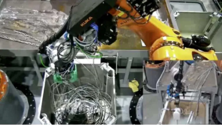
Cleaning up the past half-century of nuclear waste in the UK alone represents the largest environmental remediation project in the whole of Europe. The nuclear waste is radioactive and comprises relatively common objects such as plastic bottles, cloth, etc., while compared to general domestic objects, there are more industrial objects such as wooden blocks, metal cans, chains, gloves, pipes, other metal objects, etc. (shown in Fig. 5). In nuclear decommissioning, the waste objects should be detected, categorized, sorted and segregated. In order to sort and segregate nuclear waste objects autonomously [1], a real-time detection and recognition approach is required.
DCNN-based methods are state-of-the-art approaches for object detection and recognition. Unfortunately, most of the existing DCNN methods rely on the large-scale annotation of training data, which may be unavailable when trying to rapidly train such methods for new applications. Our work is motivated by the problem of training an RGB-D object detec-tion and recognidetec-tion system for guiding a robot manipulator
1
Extreme Robotics Lab, University of Birmingham, Birmingham, B15 2TT, UK [email protected], 2
Lincoln Centre for Autonomous Systems, University of Lincoln, Lincoln, [email protected],
∗
The corresponding author
Fig. 1. In this figure, a robot is sorting nuclear waste (metal strings and chains) into a segregation bin through teleoperation.
in handling of hazardous nuclear waste (see Fig. 1), which may contain a vast array of different kinds of objects and materials, where massive acquisition and human-annotation of training data is not practical. To overcome this problem, we first employ a model-free 3D detector to detect objectness proposals in 3D, and transfer the 3D proposals to 2D for object category recognition. Once an objectness proposal is categorized, we project the 2D classified proposal back to 3D to get a boundary-aware detection result. In our approach, bounding-box annotations are not required and boundary-aware detection is achieved. This is achieved through weakly-supervised deep learning for RGBD-based object detection.
The weakly-supervised deep learning problem has a high-dimentional feature space but sparse training examples. In order to interpolate the sparse feature points in the high-dimensional space, our neural network architecture (DCNN-GPC) combines parametric models (a multi-modal DCNN for RGB and D modalities) with non-parametric Gaussian Process Classification (GPC). Our system is trained initially using a small amount of labeled data (about 0.3%), and then automatically propagates labels to large-scale unlabeled data. More specifically, we first run 3D-based objectness detection on RGB-D videos to acquire many unlabeled object proposals, and then employ DCNN-GPC to label them. As a result, our multi-modal DCNN can be trained end-to-end using only a small number of human annotations. In this paper, a real-time detection and recognition pipeline is thus implemented for nuclear waste simulant detection and recognition.
The main contributions of this paper are threefold.
detection and recognition of real-world RGB-D nuclear waste simulants. The previous research [2] is only able to detect and recognize known nuclear waste objects, however, our proposed approach is the first deep learning-based visual perception solution for nuclear waste decom-missioning, which can detect and categorize unknown waste objects in real-time. A video demonstration of the approach is available at https://youtu.be/7w6oqfvkub0
• Secondly, our approach is weakly-supervised, in which a non-parametric GPC is used for the label propagation in order to enhance robustness to the sparsity of training data. In particular, our approach does not require bound-ing box object annotations and boundary-aware detections can be obtained.
• Thirdly, we introduce a new industrial dataset, i.e.
Birm-ingham nuclear waste simulants dataset1to be used by the
research community, which comprises a series of RGB-D videos of realistic nuclear waste-like objects.
The remainder of this paper is organized as follows: Sec-tion II gives an overview of the related literature; SecSec-tion III introduces Gaussian Process Classification (GPC) as the pre-liminary knowledge; Section IV presents the pipeline of the proposed method; Section V presents the experimental results on two real-world datasets; and the paper is concluded with contributions and suggestions for future research.
II. RELATEDWORK
In this section, we firstly review RGB and RGB-D object detection in Section II-A, and RGB-D object recognition in II-B. Then the existing achievements of weakly-supervised deep learning are introduced in Section II-C. We also review the existing research on nuclear waste detection and recogni-tion in Secrecogni-tion II-D. Finally, we give our discussion in Secrecogni-tion II-E.
A. Objectness and object detection
Most object detection literature addresses only 2D RGB images, e.g. [3], [4]. Region-based CNN (R-CNN) [5] frame-works comprise: objectness detection, then pre-trained-CNN-based feature extraction, followed by SVM classifiers for object category recognition. More recent work, [6], [7], [8], achieves greater speed by using DCNNs, in which both detec-tion and recognidetec-tion can be learned jointly and deployed in a single shot. However, DCNNs depend on large-scale human-annotated training data, which are often unavailable in real-world applications. Furthermore, these methods are based on bounding-box detection and cannot achieve boundary-aware detection.
Comparatively little literature has addressed the use of 3D data, which can greatly facilitate objectness detection by providing more salient boundaries between foreground objects and background regions. Gupta et al. [9] adapted a 2D mechanism to RGB-D without consideration of the real 3D distance metric. [10] detected 3D objects in a point cloud by applying a cuboid-shaped sliding window. [11] extended
1https://sites.google.com/site/romansbirmingham/
the region proposal networks of [12] to achieve faster object detection than sliding-shape approaches. However, these meth-ods typically generate thousands of objectness proposals for each image, making subsequent object category recognition difficult to achieve in real-time.
Alternatively, unsupervised 3D segmentation (clustering) [13], [14] can be used for RGB-D objectness detection, and can also achieve boundary-aware detection. Folkesson et al. [15] proposed a multi-view object segmentation approach with RGB-D data, where Statistical Inlier Estimation (SIE) is used to enhance the robustness of object segmentation. Such methods engender a trade-off between segmentation accuracy and speed. In our approach, we simplify the 3D clustering connectivity, using only three cues, to enable real-time perfor-mance while still achieving boundary-aware detection.
B. RGB-D object recognition
Multimodal DCNNs [16], [17], [18], [19], [20] are now widely used in RGB-D object recognition. These multimodal architectures comprise two nets (for RGB and D modalities) which are fused in the last fully-connected layers and trained jointly. These methods pre-trained both DCNNs on ImageNet, since no large-scale labeled depth dataset was available for pre-training. Unfortunately, network parameters pre-trained on RGB images (i.e. ImageNet) do not work well for raw depth data. Most methods transfer the depth modality to RGB through color-mapping [16], [17], [21], or to low-level features [19], [20], [22], to fit into a DCNN pre-trained on RGB data (ImageNet). These methods need extra computation for color-mapping and feature extraction, and the raw depth data is not fully leveraged. In contrast to previous work, our DCNN is directly trained on raw depth maps. No costly data conversions (from depth to RGB) are required, and depth information is fully exploited.
C. Weakly-supervised deep learning
Following the success of highly data-driven DCNN meth-ods, the problem of reducing annotation effort has attracted increasing attention. [20] proposed semi-supervised learning approaches for RGB-D object recognition, in which co-training methods are used to incrementally label the unlabeled data. [23] proposed a weakly-supervised DCNN to learn pixel-wise semantic segmentation from bounding-box annotations. In their method, a dense CRF is used to obtain segmentation estimations for training the DCNN.
[24] used the temporal correlation in driving videos to learn path proposals for autonomous driving. In their method, the path in future frames is projected to the current frame through vehicle odometry and annotated as ground truth for learning. [25] proposed a self-supervised approach to learn fully-convolutional networks for object segmentation in the Amazon picking challenge.
The key step in semi-supervised or weakly-supervised learning for object recognition is to model the predictive probability. In [20], the DCNN trained from labeled examples is used as the classifiers for co-training. However, small-scale training examples open up the possibility of over-fitting, and
as a consequence, a good predictive probability cannot be guaranteed. In contrast to the existing methods, we adapt non-parametric GP classification with fusion of multi-modal kernels, which is more robust to the scale of training data. We reduce the required label percentage from 5% [20] to 0.3% (at the same frame rate). More importantly, the previous research [20] focuses on recognition trained by bounding-box annotations, whereas our research is weakly-supervised with the integration of objectness detection, learned by detected objectness proposals.
D. Nuclear Simulant Detection and Categorization
Compared to existing approaches for detection and recog-nition of domestic objects, nuclear waste object detection has limited literature. Shaukat et al. [2] first applied computer vision methods to detect and recognize nuclear waste objects. Their approach is based on the grayscale image, in which shape-based histogram thresholding is employed to segment the waste object from the table. Then invariant moments are used for the feature extraction, and a random forest is trained for classification. The existing research focuses on recognizing specific waste objects rather than object categorization.
E. Discussion
Compared to 2D-based detection methods [3], [12], [6], [7], [8], [12], 3D-segmentation-based detectors can reduce the number of object proposals from thousands to less than a hundred per image. More importantly, boundary-aware de-tection can be obtained. In our approach, we propose a 3D segmentation method which is multi-cue, but more efficient than [13], for real-time objectness detection in RGB-D data.
Multi-modal DCNNs achieve state-of-the-art performance in RGB-D object recognition. However, how to fully leverage the depth modality remains a problem. Recent work [17], [19], [20], [22] assumes that raw depth images cannot be directly used to train a DCNN, because no large-scale depth dataset is available for pre-training. In contrast, we show how raw depth data can be fully leveraged, by using 3D CAD models (e.g. ModelNet dataset) to generate large numbers of automatically annotated depth images for pre-training. As a consequence, color-mapping methods and low-level depth features are not required in our approach.
Most DCNN-based detection and recognition methods are fully supervised, trained by massively annotated datasets. In contrast, weakly-supervised deep learning has, so far, only achieved success in very few applications, including path planing [24] and the Amazon picking challenge [25]. In contrast, this paper shows how weakly supervised deep learn-ing can achieve very strong performance in RGB-D object detection and recognition, at time frame rates, on real-world industrial image data, for which only a tiny amount (0.3%) of labeled data is available for training.
III. PRELIMINARIES A. Gaussian Process Classification (GPC)
Unlike popular classifiers, e.g. SVM, GPC is fully Bayesian and can generate predictions within the same distribution
for multi-class cases. Our use of GPC is as follows [26]. Given a classification problem with training instances X, training labels y, testing instance x∗, testing label y∗, and
latent variables for training and test instances f and f∗, the
GPC infers the conditional predictive probability of the test instance’s labely∗ givenX andy:
P(y∗|x∗, X, y) =
ZZ
P(y∗|f∗)p(f∗|f, x∗, X)p(f|X, Y)df∗df.
(1)
where P(y∗|f∗) is the likelihood function for classification
(which can be the logistic function for binary classifica-tion or softmax funcclassifica-tion for multi-class classificaclassifica-tion), and
p(f∗|f, x∗, X) is a standard noise-free regression. The key
problem of GPC is to estimate the posteriorp(f|X, y):
p(f|X, y) =R P(f|X)P(y|f)
P(f|X)P(y|f)df (2)
whereP(f|X)is the prior andP(y|f)is the likelihood. Here, the prior is Gaussian, whereas the likelihood is non-Gaussian, which makes Eq. 2 analytically intractable. Researchers have proposed different ways to solve this non-conjunction prob-lems, including Laplace Approximation, Expectation Propa-gation, etc. [26]
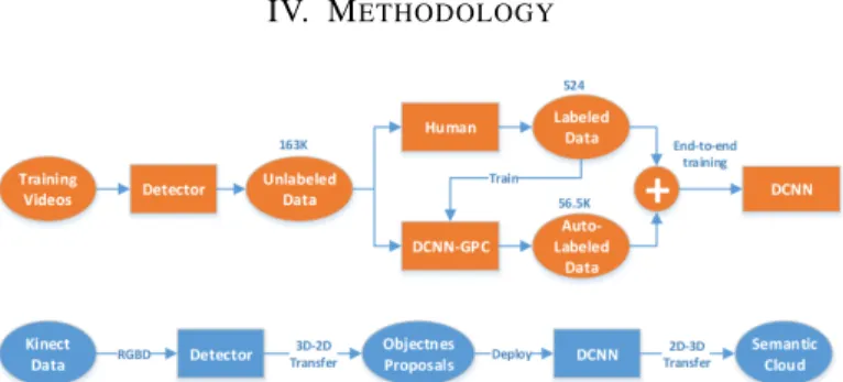
IV. METHODOLOGY
Fig. 2. Flow chart of our proposed weakly supervised DCNN method. In this chart, the training process is shown in orange and deployment in blue.
Our proposed pipeline has three steps: (1) a real-time 3D-based object detection approach is proposed to generate high-quality objectness proposals in RGB-D video streams; (2) DCNN-GPC is proposed to propagate small-scale labeled data, i.e. 1-2 examples for each training object, to moderate-scale in order to train the multi-modal DCNN end-to-end; (3) a real-time detection and recognition system is integrated.
A. Real-time 3D Objectness Detection
Our object detection approach is 3D-based and unsuper-vised, employing point cloud segmentation to obtain salient objectness (regions) proposals. We first detect large planes (using RANSAC) in point clouds and remove them, as we are interested in table-top or ground-top objects. Inspired by the multi-cues idea of [13], we propose a more efficient condi-tional clustering approach based on color, shape and spatial cues to acquire objectness proposals. Given two voxels p1
andp2, the connectivity between themC(p1, p2)is defined by distance connectivityCd(p1, p2), color connectivityCc(p1, p2) and shape connectivityCs(p1, p2):
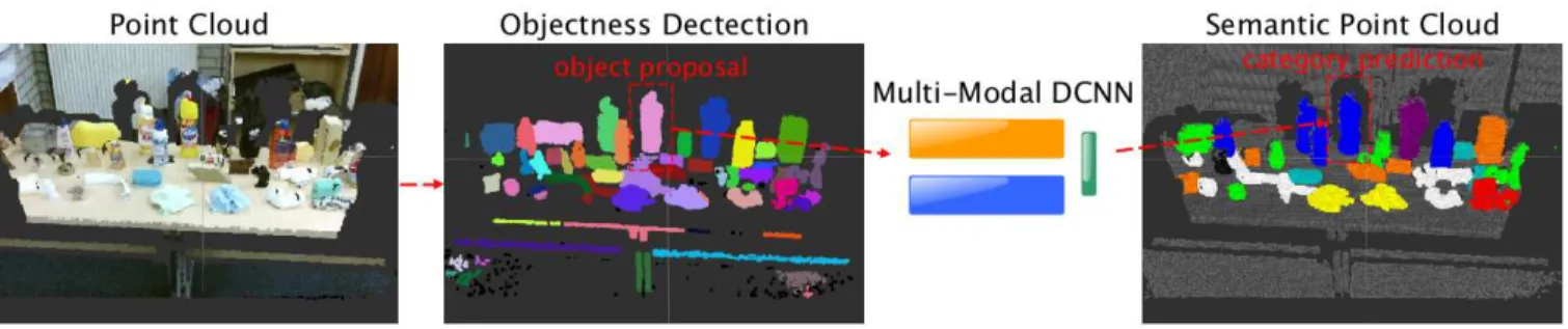
Fig. 3. Detection and recognition pipeline of our system. RGB-D point cloud (left) yields objectness proposals (middle). For each such proposal, the multi-modal DCNN performs category recognition. The pixel-wise recognition result is projected to obtain a 3D semantic point cloud.
Cs(p1, p2) = 1, if np1·np2 knp 1 kknp2k < σs 0, otherwise Cc(p1, p2) = ( 1, if kIp1−Ip2 k< σc 0, otherwise Cd(p1, p2) = ( 1, if kp1−p2k< σd 0, otherwise C(p1, p2) =Cd(p1, p2)∩(Cs(p1, p2)∪ Cc(p1, p2)) (3) where np1,np2 are the surface normals, Ip1, Ip2 refer to the intensity values of p1, p2, andσd,σc,σs are the connectivity thresholds. The neighboring voxels will be clustered iteratively through this connectivity criteria until all clusters become constant. Parameter values σd, σc, σs are set as 2 cm, 8.0 and 10◦, which perform well for our application.
Given 3D objectness proposals detected in 3D world co-ordinates, each point in the proposal p(xw, yw, zw) can be back-projected to its 2D image coordinates (u, v) and depth
d: d u v 1 =C R t 0 1 xw yw zw (4)
where C is the camera intrinsic matrix, and R and t are the rotation matrix and translation vector, respectively. In this case, a 2D bounding box with boundary-aware segmentation can be formed for each 3D objectness proposal, which is used for learning in the following section.
B. Weakly-Supervised Multi-Modal DCNN for RGB-D Object Recognition
Similar to popular DCNN-based methods [16], [17], [18], [19], [20], our recognition DCNN is also of multi-modal architecture (RGB-Net and Depth-Net for RGB and depth modalities, respectively). However, we propose a different DCNN architecture and a novel weakly-supervised method to train it, comprising three stages. First, the DCNNs are pre-trained on public large-scale datasets (ImageNet dataset for the RGB-Net and ModelNet dataset for the Depth-Net). Second, the DCNN-GPC is trained and then employed to classify large-scale unlabeled objectness proposals according
to the predictive probabilities of the GPC. Third, the multi-modal DCNN, used in the DCNN-GPC, is fine-tuned jointly end-to-end using moderate-scale automatically labeled RGB-D data.
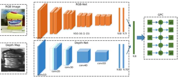
1) Network Architecture: In contrast to Caffe-Net[27] (used in [16], [17], [18], [19], [20]), we use a deeper architecture for RGB-modality recognition. That is, the VGG 16-layer architecture [28] is used for our RGB-Net with the removal of the soft-max layer. For Depth-Net, we devised an 8-layer DCNN. Compared to the widely-used Caffe-Net, our Depth-Net adapts smaller filter sizes and larger numbers of filters. The Local Response Normalization (LRN) layers [29] are applied to the first two convolutional layers’ features in order to capture the local 3D shape of the object from the relative range difference. In other words, we use LRN to transform the absolute depth to relative depth, which prevents the DCNN from over-fitting to a specific range of depth. All convolutional layers and fully connected layers are initialized by Xavier initialization [30]. The parameters of this architecture are set according to experimental experience (shown in Fig. 4 and Table I).
2) Pre-training of Multi-modal DCNN: In order to elim-inate over-fitting, pre-training is necessary. Our RGB-Net is pre-trained on ImageNet [31]. In well-known methods [16], [17], [18], [19], the DCNN for depth-modality recognition is also pre-trained on ImageNet, requiring color-mapping or low-level features to transform the raw depth data into the RGB domain. In contrast, our proposed Depth-Net is pre-trained on the Model-Net dataset [32] from scratch, by projecting many synthetic depth maps. As a result, no extra pre-processing (color-mapping or low-level features) is needed.
In our approach, we use 40 class subsets of Model-Net (in total 9.8K models) for training. For each 3D model, we sample 4×10⁴ points uniformly on the object surface and
apply white noise on those 3D points. Then for the point cloud of each object, we generate 30 camera poses, distributed on a hemisphere, and capture depth maps from each camera pose2. After 6DOF camera poses are obtained, for each camera
the inverse transform is applied to the original point cloud to transfer 3D points from world to camera coordinate systems. Hidden points removal [33] is then applied on the 3D points, 2More specifically, the poses of virtual cameras are obtained by discretizing
Euler angles: roll are 270◦, 240◦, 210◦, pitch is fixed at 0◦, and yaw are
Fig. 4. The architecture of proposed multi-modal DCNN-GPC. The inputs of the DCNNs are the raw RGB and depth images of the object proposal. Our architecture consists of three components: RGB-Net (shown in yellow), Depth-Net (shown in Blue) and non-parametric GPC (shown in Green).
and a depth image is generated by projecting visible 3D points to the image plane via Eq. 4 3. Finally, 290K depth maps are
obtained from the training models.
TABLE I
THENEURALNETWORKARCHITECTURE OF OURDEPTH-NET. layer
name
filter size number of output
other parameters conv1D 5×5 128 stride=2, pad=2, group=1
pool1 3×3 – type=max, stride=2, pad=1
norm1 5×5 – alpha=5×10⁻⁴beta=0.75 conv2D 5×5 256 stride=1, pad=2 , group=1
pool2 3×3 – type=max, stride=2, pad=2
norm2 5×5 – alpha=5×10⁻⁴beta=0.75 conv3D 3×3 384 stride=1, pad=1, group=2
pool3 3×3 – type=max, stride=2, pad=2
conv4D 3×3 512 stride=1, pad=1, group=1
conv5D 3×3 512 stride=1, pad=1, group=1
pool4 3×3 – type=max, stride=2, pad=2
fc6D – 4096 dropout = 0.5
fc7D – 4096 dropout = 0.5
fc8D – c –
3) Label Propagation through DCNN-GPC: As shown in Fig. 4, DCNN-GPC incorporates pre-trained DCNNs (with softmax layer removed) and non-parametric GP classification. That is, the outputs of the DCNNs (i.e. f c7I ∈ R4096 and
f c7D ∈R4096) are concatenated as the inputX (∈R8192) to the GPC. In this stage, we label a small number of cropped images from detected objectness proposals, and train GPC on them.
More specifically, the training data of our proposed method are unlabeled RGB-D videos. We capture the videos in a con-trolled environment, i.e. only one object category is recorded in each video. By deploying the proposed detector to the training videos, for each category, a large-scale unlabeled objectness proposals set {SU} can be obtained. We then manually label a very small sub-set {SL
m} of objectness proposals and train GPC on {SL
m}.
3In our implementation, the optical center of our virtual camera is set as
(250, 250), and focal length is 500. Consequently, a depth map of 500×500
resolution is obtained. We resize the depth maps to (224,224) for training.
In our approach, the binary GPC is adapted, and can easily be extended to multi-class GPC if the environment is not controllable. More specifically, the prior P(f|X)is modeled as Gaussian N(0, K), where K is the covariance matrix of all training examples X. In order to interpret features from different modalities, we treat the kernel as the product of kernels of different data domains:
More specifically, the priorP(f|X)is modeled as Gaussian
N(0, K), where K is the covariance matrix of all training examples X. In order to interpret features from different modalities, we treat the kernel as the product of kernels of different data domains:
k(x, x′) =kI(xI, xI′)∗kD(xD, x′D) (5) where x(I,) is the first 4096-dimensional feature vector pro-duced by f c7I of RGB-Net andx(D′) refers to the last 4096-dimensional feature vector produced byf c7D of Depth-Net,
x= [x(I′), x(D′)]. In our approach, an RBF kernel is used for
k1 andk2:
kRBF(x, x′) =α2exp
−kx−x′ k
2β2 , (6)
The scale parameterαand deviation parameterβ are hyper-parameters of the kernel. Consequently, k has four hyper-parameters.
In order to solve this non-conjugate problem in the posterior estimation of the GPC, Laplace Approximation [26] is used in our approach. The posterior P(f|X, y) in Eq. 2 can be modeled as a multi-variant Gaussian and we approximate the mean and Hessian of this Gaussian distribution through the Gaussian-Newton method. More details of the Laplace Approximation are given in Section VI.
Moreover, the hyper-parameters mentioned above are opti-mized through maximizing the log marginal likelihood (the log of the denominator of Eq. 2). As investigated in our previous research [34], this step is of significant importance, as the predictive probability can be well-spread after hyper-parameter optimization. In this paper, the
Broyden-Fletcher-Goldfarb-Shanno algorithm (BFGS) [35] is employed for the optimization. BFGS is a first order derivative-based optimiza-tion method in which the partial derivative of the marginal likelihood with respect to the hyper-parameters is required (calculated by Eq. 20). More details on the estimation of hyper-parameters can be found in Section VI.
After the GPC is trained and hyper-parameters optimized, we employ GPC to propagate labels to the large-scale unla-beled dataset {SU}. We model the prediction confidence as the predictive probability of GPC:
conf idence=P(y∗|x∗, X, y) (7)
We set a confidence interval ∈ [τ,1] and assign an object label to those examples whose prediction confidence lies in this interval, yielding a moderate-scale of labeled data{SL
GP}.
4) End-to-End Training using DCNN-GPC Labeled Data:
Having large-scale unlabeled data automatically labeled by DCNN-GPC, sufficient training examples, i.e. {SL
m} and {SL
GP}, are obtained to train RGB-Net and Depth-Net from-end-to-end. At this stage, we replace GPC with a softmax loss layer, connected with fully-connected layer f c8. We extend the conventional multi-modal softmax loss (i.e. negative log likelihood) [17] to the weakly-supervised case:
loss=− X i∈SL m
logL(sof tmax(ff c8
([Of c7I i , O f c7D i ], θ f c8 )), yi) −η X j∈SL GP
logL(sof tmax(ff c8([Of c7I j , O f c7D j ], θ f c8 )), yj) (8) whereOf c7I(D)
∗ is the output off c7I(D),Lis the likelihood function,θis the weight vector off c8, andyi(j)refers to the
training label. η ∈ [0,1]is the penalty factor of the DCNN-GPC automatically labeled training data, set according to the automatic annotation quality. In our implementation, the loss of DCNN-GPC-labeled examples is treated equivalently to that of manually-labeled examples (η=1.0), as our DCNN-GPC yields satisfactory annotations.
It is worth noting that our DCNN-GPC is end-to-end trainable as the DCNN and GPC can be implemented as tensors. While from our experiments, we find that, via min-imizing negative log likelihood of the GPC, the end-to-end training suffers from local minima. A more practical way is to freeze the DCNN and train the GPC when very small-scale training examples are available. Once the moderate-scale examples are annotated, we find that GPC cannot further advance the classification result but slows down the forward-propagation inference (because the computation of the non-parametric models positively propagates to the number of training examples). In this paper, GPC is only used for label propagation in the weakly-supervised learning and we directly use the softmax layer output for straight-forward deployment.
V. EXPERIMENTS
We report the following two sets of experimental results. It is worth noting that our proposed detection pipeline is weakly-supervised as image-level annotations (i.e. cropped im-ages) rather than bounding-box annotations are required. The
proposed DCNN-GPC can be used standalone (without 3D objectness detection) for semi-supervised object recognition.
In Section V-B, we first evaluate the performance of our semi-supervised DCNN-GPC for RGB-D object recognition using the Washington RGB-D object recognition benchmark4
[36]. We further evaluate the effectiveness of our proposed weakly-supervised RGB-D object detection pipeline for a novel real-world application, using our new dataset of indus-trial objects (nuclear waste simulants) in Section V-C.
A. Pre-training
Before the two experiments, for initialization, the weights of RGB-Net and Depth-Net are pre-trained on the ImageNet and ModelNet datasets, respectively. More specifically, we directly transplant the weights of the standard VGG16 ImageNet model to RGB-Net. Then, we pre-train the proposed Depth-Net on the 40-class subset of the Princeton Model-Net dataset5. There
are 12.4K 3D CAD models in total (9.8K for training, 2.4K for validation). Following the procedure illustrated in Section IV-B2, 290K depth maps are obtained from the training models.
Since our goal is to utilize Model-Net dataset to pre-train our Depth-Net (not to optimise 3D model classification to maximise performance on the Model-Net challenge), in our approach, we minimize the average negative log likelihood of all 2.5D views. A mini-batch of 128 is used for learning with Stochastic Gradient Descent (SGD). The learning rate is set to 0.01 with a reduction of 10 times every 10K iterations. Training converges after 30K iterations. The momentum is fixed to 0.9 and weight decay is 5×10⁻⁴.
B. Washington RGB-D Object Recognition Dataset
TABLE II
COMPARISON WITH TOP-RANKING METHODS ON THEWASHINGTON RGB-DDATASET. THE ACCURACY IN THIS TABLE IS OF%. Supervised Methods RGB Depth RGB-D CNN-RNN[37] 80.8±4.2 78.9±3.8 86.8±3.3 Upgraded HMP[38] 82.4±3.1 81.2±2.3 87.5±2.9 Multi-Modal[17] 84.1±2.7 83.8±2.7 91.3±1.4 Hypercube Pyramid[39] 87.6±2.2 85.0±2.1 91.1±1.4 STEM-CaRFs[14] 88.8±2.0 80.8±2.1 92.2±1.3 (DE)2CO [40] 89.5±1.6 84.0±2.3 93.6±0.9 RCFusion[41] 89.6±2.2 85.9±2.7 93.9±1.0 Semi-supervised Method RGB Depth RGB-D Semi-CNN-RNN [42] 77.1±2.3 71.8±0.8 81.6±1.4 Semi-CNN-SPM-RNN [43] 78.7±1.4 75.4±2.4 83.7±1.3 Semi-DCNN [20] 85.5±2.0 82.6±2.3 89.2±1.3 Ours 86.2±2.6 76.3±2.5 90.2±1.7
The Washington RGB-D object dataset comprises 300 objects organized in 51 categories. In this experiment, the evaluation set (a subset of every 5 frames, giving a total of 41,877 RGB-D images) reported in Lai et al. [44] is used. We follow the original training/validation splits. It is worth noting that objectness-detection is not included in the Washington dataset, hence only semi-supervised recognition i.e. DCNN-GPC is evaluated in this experiment.
4https://rgbd-dataset.cs.washington.edu/ 5http://modelnet.cs.princeton.edu/
Following the experimental evaluation reported for existing semi-supervised methods [43], [20], we also randomly select 5% (approximately 1,750) of the training examples as labeled and the rest as unlabeled. We train our proposed DCNN-GPC with the labeled examples and automatically annotate the remaining 95% of unlabeled examples. Then the DCNN can be trained end-to-end with a moderate number of automatically annotated examples.
More specifically, we initialize the DCNN and train the GPC on the 5% labeled data and then employ the trained system to classify the remaining 95% unlabeled data. The examples with high predictive probability are moved from the unlabeled set {SU} to the GP-labeled set {SL
GP}. After the label propagation, approximately 60K of 166K unlabeled examples are automatically annotated. In this step, we found that the recognition performance is robust to the confidence interval (∈[τ,1]) parameter τ in the range between 0.5 and 0.8. We chose τ as 0.7 for the best performance. Moreover, we also evaluated a different label propagation strategy, that is, incrementally propagating the labels to instances with highest predictive probability, however, there was little improvement but significantly higher time consumption with this approach. Therefore, a single batch label propagation strategy is used as a trade-off between effectiveness and efficiency.
Having unlabeled instances automatically annotated, our multi-modal DCNN can be trained end-to-end in three steps. Firstly, we freeze the RGB-Net layers and fusion layers (disable sof tmaxf usion), and finetune the Depth-Net with mini-batch of 64, fixed learning rate 10−2 and weight
de-cay 5×10⁻⁴. This training converges after 20K iterations.
Secondly, we fine-tune both RGB-Net and Depth-Net (still disabling sof tmaxf usion) with mini-batch of 32 and fixed learning rate 10−3 for another 10K iterations. Finally, similar
to [17], we freeze the RGB-Net and Depth-Net layers and train the fusion layer. A mini-batch of 32 and fixed learning rate 5×10⁻⁴ are used, and training converges quickly after 5K
iterations. We repeat this experiment ten times following the original training/validation splits and the mean accuracy and standard deviation are calculated.
As shown in Table II, our semi-supervised DCNN-GPC achieves an average recognition accuracy of 86.2% for RGB, 76.3% for depth and 90.2% for RGB-D among 51 categories of objects, which outperforms all compared state-of-the-art semi-supervised approaches [42], [43], [20]. In contrast to these parametric model based methods, non-parametric Gaussian Process Classification is used in our approach, which has the potential to be learned from fewer labeled training examples. Moreover, we also train our DCNN in a fully supervised form on all the examples, and the performance (average accuracy) is 88.4% for RGB, 80.8% for depth and 91.8% for RGB-D. Compared to fully-supervised DCNN (91.8%), our weakly-supervised DCNN-GPC achieves a slightly lower result (90.2%) using only 5% of training examples. This result demonstrates the effectiveness of our DCNN-GPC for label propagation.
Compared to other DCNN methods [16], [17], [18], [19], [20], we use a deeper architecture for the RGB modality, thereby achieving better RGB recognition performance.
More-Fig. 5. Some examples from the Birmingham nuclear waste simulants dataset.
over, unlike other methods, our Depth-Net uses raw depth data for training, i.e. real end-to-end learning between raw sensor data and the learning objective. Inference of the depth modal-ity is more straightforward as no extra computation (color mapping or low-level features) is required. For comparison, dense surface normal extraction6 takes 1.5-3.0 seconds per
depth image after down-sampling to 0.5 cm voxel size and 0.3-0.7 second with 1 cm voxel size. HHA encoding has higher computation complexity as it is based on surface normals. Our approach does not require depth data pre-processing, which makes the real-time application possible. Moreover, our multi-modal DCNN is pre-trained on different types of data, and more distinctive classification views are trained for different modalities. Though the performance of our depth-Net is lower than the state-of-the-art, substantial improvement is then obtained by fusing multi-modal DCNNs.
C. Real-world Nuclear Waste Simulants Recognition using Weakly Supervised Learning
In this experiment, we evaluate the whole RGB-D object detection/recognition pipeline in contrast with RGB-D ob-ject classification. In today’s real-world applications such as nuclear waste object detection and recognition, large-scale bounding-box annotations are not practical. The state-of-the-art semi-supervised RGB-D recognition method [20] does not
TABLE III
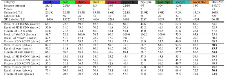
STATISTICS OF OURNUCLEAR STIMULANT OBJECT DATASET,TRAINING EXAMPLES,AND QUANTITATIVE RESULTS OF OUR PROPOSED DETECTION/RECOGNITION SYSTEM. DETECTION PRECISION RATE,RECALL RATE AND F-SCORE OF EACH CATEGORY ARE GIVEN. T.E.STANDS FOR TRAINING EXAMPLES,PRESCI.FOR PRECISION,INST.W.FOR
INSTANCE-WISE,PIX.W.FOR PIXEL-WISE, OVE.FOROVERALL ANDAVE.FORAVERAGE.
Category bottles cans chains cloth gloves metal obj. pipe join. plas. pipe sponges wood bloc. Ove./Ave. Instance Amount 28/12 22/15 8/3 6/3 16/5 22/10 9/5 10/4 12/6 14/7 147/70 Videos 4 2 2 4 4 4 2 2 2 3 23 Unlabelled T.E. 20.5K 32.5K 18.3K 13.3K 8.6K 22.1K 21.9K 8.0K 9.0K 14.0K 163K Labelled T.E. 48 56 26 45 35 48 28 20 32 32 524 GP Labelled T.E. 11436 15525 2322 4606 5298 6101 2287 1037 3223 4734 56.5K Preci. of 3D R-CNN (inst.w.) 68.1 72.6 69.8 62.3 48.9 60.0 44.6 72.2 62.3 67.9 64.6 Recall of 3D R-CNN (inst.w.) 53.0 71.0 79.0 70.2 41.8 50.9 45.2 46.4 53.5 17.0 52.3 F-Score of 3D R-CNN 59.6 71.8 74.1 66.0 45.1 55.1 45.0 56.5 57.6 27.1 57.8 Preci. of YoloV3 (inst.w.) 38.7 52.1 100.0 76.5 90.9 100.0 100.0 100.0 73.3 95.8 55.1 Recall. of YoloV3 (inst.w.) 47.5 51.0 17.1 28.9 17.9 9.8 6.3 20.3 34.4 20.0 30.5 F-score of 3D RCNN (pix.w.) 42.7 51.5 29.2 42.0 29.9 17.9 11.9 33.7 46.8 33.1 39.3 Preci. of ours (inst.w.) 89.2 81.8 79.2 93.3 68.3 75.0 66.7 63.2 92.5 87.8 80.9 Recall of ours (inst.w.) 83.2 91.8 95.0 80.0 91.5 64.0 90.2 50.0 87.5 87.8 83.5 F-Score of ours (inst.w.) 86.1 86.6 86.4 86.2 78.2 69.1 76.7 55.8 89.9 87.8 82.2 Preci. of 3D R-CNN (pix.w.) 66.8 63.6 68.1 58.0 55.2 45.4 57.3 43.8 55.1 59.4 59.5 Recall of 3D R-CNN (pix.w.) 47.5 58.9 48.6 56.8 35.0 36.3 53.0 10.2 45.2 13.4 42.1 F-score of 3D RCNN (pix.w.) 55.5 61.1 56.7 57.4 42.8 40.4 55.1 16.6 49.7 21.9 49.3 Preci. of ours (pix.w.) 83.2 70.2 76.0 89.6 67.0 70.0 62.0 60.6 84.3 86.9 75.5 Recall of ours (pix.w.) 75.4 70.9 66.2 70.8 75.1 48.6 85.4 37.1 68.4 72.7 70.4 F-Score of ours (pix.w.) 79.1 70.6 70.8 79.1 70.8 57.3 71.8 46.0 75.5 79.1 72.9
provide the detection pipeline, and reproducing and optimizing the training process on our dataset is unlikely to be possible (source code is not published for [20]). Therefore, we only compare with [20] on the Washington benchmark.
1) Baseline Methods: In this experiment, we implement two baseline methods for comparison. In order to investigate the advances of our proposed method, we compared our method with both two-stage and end-to-end methods.
• 3D R-CNN. R-CNN [5] is a classic two-stage detection
approach which has fair performance but low frame rate. In R-CNN, a 2D-based object proposal method is used for objectness detection, with a pre-trained VGG-16 Net for feature extraction and SVM for classification. In our implementation, we upgrade the 2D-based object proposal method to our proposed 3D objectness detection. As a result, the running time of the whole detection pipeline can be significantly boosted.
• Yolo v3 [45]. Compared to the previous end-to-end detection methods, e.g. Yolo [7] and SSD [8], Yolo v3 is faster and stronger. We use the Darknet-53 model with 416×416 images for this experiment. The base network is pre-trained on the ImageNet dataset. For a better performance, we use a ratio of 1:3 to feed positive and negative bounding boxes in the training procedure. We use a confidence of 0.25 to filter the detected objects. All above parameters are set according to our practical experience.
The two baseline methods are trained by using manually labeled objectness proposals. This comparison aims to show the advances of our proposed weakly-supervised DCNN over supervised approaches, e.g. 3D R-CNN and Yolo v3, when very few labeled data are available.
It is worth noting that we did not compare with instance segmentation methods such as Mask-RCNN [46]. The reason is two-fold: first, the mechanism of our proposed method is an RGB-D based detection pipeline, and the boundary-aware results can be obtained by 3D-based objectness detection
rather than image-based semantic segmentation; second, our dataset provides image-level annotation and bounding-box an-notation for training, however, the pixel-wise boundary-aware annotation is not available. Therefore, we only compared with detection methods, i.e. 3D R-CNN and Yolo v3.
2) Dataset: In order to evaluate our proposed weakly-supervised deep learning approach for nuclear waste object de-tection and recognition, we created a novel dataset comprising videos and models of nuclear waste simulants7. In contrast to most other RGB-D recognition challenges (typically involving household or office objects), our application focuses on the major societal problem of robotic decommissioning and clean-up of nuclear waste, which involves an enormous variety of contaminated objects and materials. In our dataset, there are 217 objects of 10 categories of objects which are common in legacy nuclear waste repositories: plastic bottles, cans, chains, cleaning cloths, gloves, metal objects, plastic pipes, pipe joints, sponges, and wooden blocks. We randomly split all instances into a training set (147 instances) and a testing set (60 instances), and all testing objects were previously unseen. Our training data are mainly RGB-D video clips in which training objects are placed on a table. In this experiment, the videos are captured by a Kinect v2 in QHD resolution (540×960). In each video, the camera trajectory covers approximately 180◦ field of view of the objects and the camera poses range from 30◦ to 60◦ above the horizon.
3) Implementation and Running Time: Our computer has an i7 8-cores CPU and a NVIDIA TITAN X GPU (12G). In our implementation, the IAI Kinect2 package8 is used to interface
with ROS and calibrate the RGB and depth cameras. Our DCNN is based on the Caffe toolbox[27]. Our entire pipeline is integrated into ROS9. The running time of our proposed detection and recognition method is 2-3HZ for a QHD point 7The dataset is available online: https://sites.google.com/site/
romansbirm-ingham
8https://github.com/code-iai/iai kinect2/ 9http://www.ros.org/
RGB image Our method (2D) Ground truth Our method (3D)
Fig. 6. The qualitative results. From left to right: RGB images, 2D semantic map of our method, ground truth, 3D semantic map of our method.
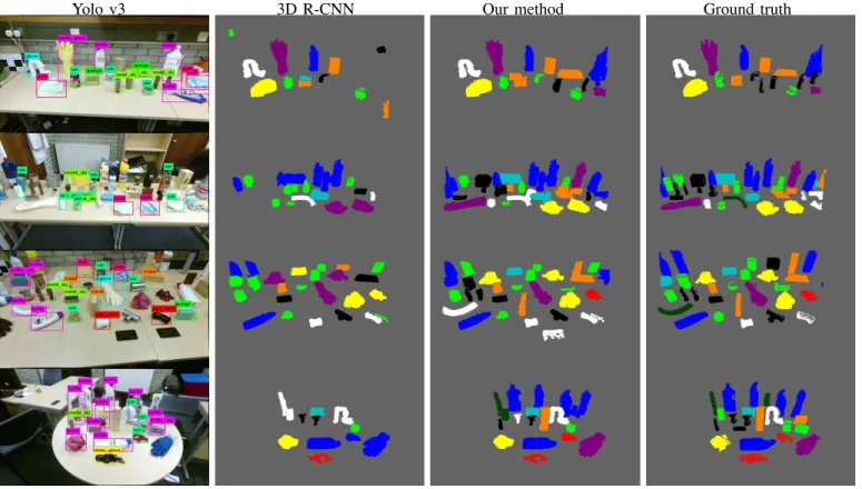
Yolo v3 3D R-CNN Our method Ground truth
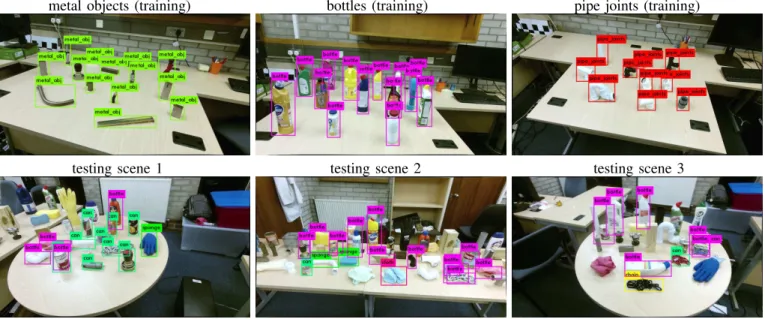
metal objects (training) bottles (training) pipe joints (training)
testing scene 1 testing scene 2 testing scene 3
Fig. 8. A deeper analysis of the results of Yolo v3. The first row shows selected results on the training images and the second row selected results on the testing data. We found that Yolo v3 suffers from over-fitting when large-scale training data is not available. As shown in the lower-middle figure, the objects with novel background are not detected. In the lower-left figure, the objects of coarse scale are not detected and objects with similar appearance are misclassified. In the lower-right figure, the cluttered objects and small objects are not detected.
cloud. The detection time is monotonically increasing with the number of 3D points. Moreover, we also devised a lighter DCNN architecture, which can run 3 times faster with only slightly lower performance. Our pipeline can be boosted to 5HZ with point cloud down-sampling and the lighter DCNN architecture. In comparison to previous state-of-the-art RGB-D object detection methods, 4 seconds per frame (0.25HZ) was achieved by [47] and 16 seconds per frame (0.0625HZ) by [11]. The performance of our method is an order magnitude greater, and can reasonably be described as near-real-time.
4) Training: 23 video clips were captured for training and 3 for testing. In each training video, training objects of a specific category were placed on a table. Each object was captured in different poses and from different viewpoints. Our proposed objectness detection approach generated 163K un-labeled object proposals. We manually un-labeled 524 examples (i.e. bounding boxes) in total, and trained a binary DCNN-GPC for each category. Statistics of our training data are detailed in Table III. Having a DCNN-GPC trained by manually labeled examples, the confidence(i.e. predictive probabilities) of the 163K unlabeled examples can be estimated by Eq. 7. If the predictive probability of an example is larger than τ, then the prediction is treated as confident and this example is assigned the label of the corresponding category, otherwise it is abandoned. In our implementation, we set τ to 0.7 for all categories. A grid search (τ ∈ [0.1, 0.9]) is used to find the optimal parameters. A stable performance can be achieved with a wide range of τ ([0.5, 0.8]). In this procedure, 56.5K of 163K unlabeled examples are automatically labeled by DCNN-GPC. Then we fine-tune our multi-modal DCNN using both GP-labeled and manually-labeled examples. For Yolo v3, we use the original DarkNet implementation10and the training
follows the standard PASCAL VOC runtime. 10https://pjreddie.com/darknet/yolo/
5) Evaluation: As the parameters of our detector are fixed, a ROC curve is not available. Instead,precision,recall
and F-score are used for evaluation. Unlike conventional bounding-box-based detection methods, our approach gener-ates boundary-aware (i.e. pixel-wise) detection results. Hence, we evaluate these three metrics for both instance-wise and pixel-wise cases. For evaluation, we first acquire keyframes from the four testing videos according to visual odometry. For each video, we uniformly select 10 frames from all keyframes. In total, 40 testing frames are obtained. We densely annotated all the objects in these 40 frames (approximately 1K objects). In the instance-wise evaluation, detections are considered as true or false positives if the overlap area between prediction and ground truth exceeds 50%. In the pixel-wise evaluation, true or false positives are counted between corresponding pix-els. Quantitative results are shown in Table III and qualitative results are shown in Fig. 6.
As shown in Table III, our approach achieves 80.9% average precision, 83.5% recall, 82.2% F-score in the instance-wise de-tection test, and 75.5% average precision, 70.4% recall, 72.9% F-score in the pixel-wise detection test. We observe that the difference between instance-wise and pixel-wise performance can be attributed to 3D clustering error, i.e. an object may be segmented as more than one cluster, and the small clusters are ignored because of their small physical dimension. Moreover, the boundary-aware detection is susceptible to point cloud down-sampling, resulting in decreased precision of object boundaries.
It is worth noting that we also implemented the cosine distance on RGB values as the color connectivity Cc(p1, p2) in Eq. 3 and we got very similar object-wise detection perfor-mance and slightly lower pixel-wise detection perforperfor-mance. That is, 74.7% precision, 68.1% recall, 71.2% F-score in pixel-wise using RGB with cosine distance. Therefore, we
use intensity (grayscale) value as the appearance clustering condition in our 3D detector.
From deeper analysis, the categories of shiny objects, e.g. metal objects and pipes, experience a lower precision and re-call (approximately 70%/55%) compared to non-shiny objects, e.g. bottles, sponges and wooden blocks (above 85%/85%). This is because the missing depth data on the shiny surface results in the reduced ability of our 3D-based detector. And those missing depth values lead to a more significant reduction in performance for pixel-wise evaluation. Moreover, a large proportion of the voxels on flat or tiny objects is likely to be misclassified as background in the plane removal step of the object detection. As a consequence, the recall rates of small or flat object categories (i.e. metal objects, cloth, gloves) are lower than for regular size objects.
6) Comparison with Baseline Methods: The results sug-gest that our weakly-supervised DCNN performs substantially better than the fully supervised 3D R-CNN and Yolo v3, when few labeled training examples are available (more than 20% above 3D R-CNN and 40% above Yolo v3 in F-Score). Compared to 3D R-CNN and Yolo v3, our weakly-supervised DCNN is more robust to scale-changes, the variance of poses and complexity of background. This is because the moderate number of automatically labeled data optimizes the DCNN end-to-end.
The 3D R-CNN achieved a lower performance than our proposed method with a precision of 64.6%, recall of 52.3%, F-score of 57.8% at the instance level, and a precision of 59.5%, recall of 42.1%, F-score of 49.3% at the pixel level. This significant reduction in performance can be attributed to the limited training examples. Without weakly-supervised label propagation, the classifier is unlikely to learn robustness to pose variance. Moreover, without end-to-end learning, the flat classifier, i.e. SVM, is unlikely to learn a good decision boundary for objects with a similar appearance. For example, as shown in Fig. 7, some wooden blocks, white plastic pipes and yellow gloves are misclassified as background.
Compared to two-stage methods, the end-to-end methods suffer from serious over-fitting when limited training examples are available. To be more specific, Yolo v3 achieves on average 55.1% precision, 30.5% recall and 39.3% F-score. This performance is significantly lower than 3D R-CNN and our proposed methods. From the failure cases shown in Fig. 8, we can find the following weakness of Yolo v3 in this experiment. First, the detection is likely to fail when the background is complex or unknown. This is because the objectness localization needs much more data to generalize, and 2D based detection is more sensitive to variance in the background than 3D-based detection. Second, Yolo v3 is more sensitive to the change of scale, while our proposed method is invariant to the image scales. Third, Yolo v3 shows lower capability in detecting small objects as an inherent limitation of its network architecture. That is, the background will be involved in the semantic feature if the size of the object is smaller than the size of the feature grid. Lastly, RGB-based categorization experiences difficulty in classifying objects with similar appearances, e.g. cans and metal objects, while our RGBD-based categorization is more robust in these cases.
VI. CONCLUSIONS
This paper proposed a novel weakly-supervised deep learn-ing approach (DCNN-GPC) for detection and recognition of nuclear waste objects. Compared to the previous research [2], our approach is based on deep learning and is able to detect and categorize unknown waste objects. In particular, our ap-proach leverages the merits of parametric and non-parametric models. That is, the parametric DCNN learns the discrimi-native features as the deep kernel of a non-parametric GPC, and the GPC can infer the multi-class predictive probabilities within the same distribution for weakly-supervised learning. The method, i.e. DCNN-GPC, is end-to-end, scalable and Bayes-based. From a practical perspective, our approach is trained using minimal annotated data (approximately 50 exam-ples for each category) by propagating minimal labels to large-scale unlabeled data. From the experiments, our proposed DCNN-GPC shows its effectiveness in handling extremely sparse training examples in the label propagation. We also proposed a novel way to pre-train a DCNN for the depth modality, by using large-scale virtual CAD data, enabling full leveraging of depth data without color-mapping or low-level features. Good adaptation from virtual data to real-world depth data has been demonstrated.
Furthermore, a real-time (several frames per second) detec-tion and recognidetec-tion pipeline has been integrated and demon-strated. Unlike previous methods, bounding-box annotations are not required in training, but boundary-aware detection is achieved. For evaluation, we created a novel industrial object dataset, i.e. Birmingham nuclear waste simulants dataset, and demonstrated that DCNNs can be weakly-supervised to effectively solve novel real-world applications.
For future works, we will investigate the possibility of proposing a more robust detection in consecutive RGB-D stream with visual odometry [48]. We will further apply the proposed object detection method to visually-guided manipu-lation [49], [50], [51] and investigate the possibility to adapt this approach to other types of data, e.g. 3D Lidar [52], [53], [54].
APPENDIX1: LAPLACEAPPROXIMATION
Following Eq. 2, from Bayes’s rule, the posterior over latent variables can be inferred by:
p(f|X, y) =p(y|f)p(f|X)/p(y|X)
∝p(y|f)p(f|X) (9) Writing into log format, we can obtain the log posterior:
Ψ(f) = logp(f|X, y)∝logp(f|X) + logp(y|f) (10) , where the prior of latent variable is a Gaussian f|X ∼ N(0, K): logp(f|X) =−1 2f TK−1f−1 2log|K| − Cn 2 log 2π (11) , andp(y|f)is modelled by the soft-max function:
p(yc i|fi) =πci = exp(fic)/ C X c′=1 exp(fc′ i ). (12)
In Laplace approximation, we compute the first order dif-ferential of log posterior p(f|X, y):
∇logp(f|X, y),∇logp(f|X) +∇logp(y|f)
=−K−1f+y−π (13)
where, ∇logp(f|X) = −K−1f and ∇logp(y|f) = y−π. π is the vector with the length of Cn, containing soft-max probabilities of every latent variableπc
i. Then, the second order differential can be obtained by:
∇∇logp(f|X, y) =−K−1−W, (14) where W is a Cn×Cn matrix containing the ∂2
∂fc′
j ∂fc
′′
k
logp(yc
i|fi), which can be calculated by:
∂2 ∂fc′ j ∂fc ′′ k logp(ycj′|fj) = πc′ j −πc ′ jπc ′′ k , if j=k, c′ =c′′ −πc′ j πc ′′ k , if j=k, c′6=c′′ 0, otherwise , (15) In the implementation, W can be obtained by calculating
diag(π)−ΠΠT, in whichΠis obtained by vertically stacking diagonal matrices of diag(πc), and πc is a sub-vector of π w.r.t category c. After the first and second order differentials are computed, the Newtown’s method is applied to find the maximum of latent variable:
fnew= (K−1+W)−1(W f +y−π). (16)
APPENDIX2: HYPER-PARAMETERSOPTIMIZATION
From Laplace Approximation, the second order Taylor expansion of the posterior p(f|X, y)is:
Ψ(f)≈Ψ( ˆf)+1 2(f−fˆ) T∇Ψ( ˆf)+1 2(f−fˆ) T∇∇Ψ( ˆf)(f−fˆ) (17) , where ∇Ψ( ˆf) is zero. Then, substituting approximated
∇∇Ψ( ˆf)(calculated by Eq.14) into the marginal likelihood, we can obtain the Laplace approximation of marginal likeli-hood: p(y|X, θ) = Z p(y|f)p(f|X, θ)df = Z exp(Ψ(f))df = exp(Ψ( ˆf)) Z exp(−1 2(f−fˆ) T(K−1+W)(f−fˆ))df (18) The Gaussian integral can be solved analytically, then the log marginal likelihood can be conducted as [26]:
logq(y|X, θ)≃ −1 2fˆ TK−1fˆ+yTfˆ− n X i=1 log( C X c=1 expfˆc i) −1 2log|ICn+W 1 2KW12| (19) In Eq. 19, since fˆ and W has implicit relationship with hyper-parameters θ, we can compute the partial derivative of log q(y|X, θ)w.r.t. θ into explicit and implicit parts.
∂logq(y|X, θ) ∂θj ≃ ∂logq(y|X, θ) ∂θj |explict+ Cn X i=1 ∂logq(y|X, θ) ∂fˆc i ∂fˆ ∂θj (20) Then the explicit part can be solve by:
∂logq(y|X, θ) ∂θj |explict= 1 2fˆ TK−1∂K ∂θj K−1fˆ −1 2tr((W −1+K)−1∂K ∂θj ) (21)
For the second term of Eq. 20, has:
∂logq(y|X, θ) ∂fˆc i =−Kfˆic+ ∂log p(y|fˆ) ∂fˆc i −1 2 ∂log|B| ∂fˆc i (22) We can utilize ∂q(f∂f|X,y) = 0 when f = ˆf, hence −Kfˆc
i + ∇log p(y|fˆc i) = 0, yielding: ∂logq(y|X, θ) ∂fˆc i =−1 2 ∂log|B| ˆ fc i =−1 2tr((W −1+K)−1∂W ∂fˆc i ) (23)
, in which W is the Cn×Cn matrix calculated by Eq.15. Then we differentiate each element of Wj,k (in jth row and
kth column) w.r.t. a specific scalarfc
i. The elements of ∂Wj,k
∂fˆc i
ifj=k=i can be calculated as follows:
(1−2πc′ j)(πc ′ j −πc ′ j πc ′′ k ), if c ′=c′′=c (1−2πc′ j)(−πc ′ j πic), if(c′=c′′)6=c −((πc′ j −(πc ′ j )2)πc ′′ k +πc ′ j (−πc ′′ k πci), if , c′ 6=c′′, c=c′ −((−πc′ jπci)πkc ′′ +πc′ j(πc ′′ k −πc ′′ k πci), if c′6=c′′, c=c′′ −((−πc′ jπci)πkc ′′ +πc′ j(−πc ′′ k πci), if c′6=c′′, c′′6=c , (24) and the rest are zeros.
In Eq. 13,∇logp(f|X, y)should be 0 whenfis at the max-imum point. As a result, we can get,−K−1fˆ+∇logp(y|f) = 0, therefore, yielding fˆ=K(∇logp(y|f)).
∂fˆ ∂θj = ∂K ∂θj ∇logp(y|f) +K∇ logp(y|f) ∂fˆ ∂fˆ ∂θj (25) Substituting: ∇logp(y|f) ∂fˆ =∇∇ logp(y|f) =W, ∇logp(y|f) =y−π, and solving Eq. 25, we can get:
∂fˆ ∂θj
= (I+KW)−1∂K ∂θj
(y−π) (26) After obtaining∂logq(y|X, θ)/∂fˆc
i and∂f /∂θˆ j by Eq. 22
and substituting them into Eq. 20, the derivative of Laplace approximated distribution can be obtained.
ACKNOWLEDGMENT
We thank NVIDIA Corporation for generously donating a high-power GPU on which this work was performed. This work was funded by EU projects H2020 RoMaNS 645582 and CHIST-ERA (Perception-Guided Robotic Grasping), and
by EPSRC projects EP/M026477/1 (UK-Korea Civil Nuclear Collaboration), EP/P017487/1 (Remote Sensing in Extreme Environments) and EP/R02572X/1 (National Centre for Nu-clear Robotics). Zhao was sponsored by DISTINCTIVE - a university consortium funded by the Research Councils UK Energy programme. Stolkin was sponsored by a Royal Society Industry Fellowship. Sun and Duckett were sponsored by EU H2020 ILIAD 732737. Sun and Liu were sponsored by National Natural Science Foundation of China No. 61803396.
REFERENCES
[1] N. Marturi, A. Rastegarpanah, V. Rajasekaran, V. Ortenzi, Y. Bekiroglu, J. Kuo, and R. Stolkin, “Towards advanced robotic manipulations for nuclear decommissioning,” inRobots Operating in Hazardous Environ-ments. InTech, 2017.
[2] A. Shaukat, Y. Gao, J. A. Kuo, B. A. Bowen, and P. E. Mort, “Visual classification of waste material for nuclear decommissioning,”Robotics and Autonomous Systems, vol. 75, pp. 365–378, 2016.
[3] J. R. Uijlings, K. E. Van De Sande, T. Gevers, and A. W. Smeulders, “Selective search for object recognition,”International journal of com-puter vision, vol. 104, no. 2, pp. 154–171, 2013.
[4] P. Arbel´aez, J. Pont-Tuset, J. T. Barron, F. Marques, and J. Malik, “Mul-tiscale combinatorial grouping,” inProceedings of the IEEE Conference on Computer Vision and Pattern Recognition, 2014, pp. 328–335. [5] R. Girshick, J. Donahue, T. Darrell, and J. Malik, “Rich feature
hierarchies for accurate object detection and semantic segmentation,” inProceedings of the IEEE conference on computer vision and pattern recognition, 2014, pp. 580–587.
[6] S. Ren, K. He, R. Girshick, and J. Sun, “Faster R-CNN: Towards real-time object detection with region proposal networks,” inConference on Neural Information Processing Systems, 2015, pp. 91–99.
[7] J. Redmon, S. Divvala, R. Girshick, and A. Farhadi, “You only look once: Unified, real-time object detection,” inProceedings of the IEEE Conference on Computer Vision and Pattern Recognition, 2016, pp. 779– 788.
[8] W. Liu, D. Anguelov, D. Erhan, C. Szegedy, S. Reed, C.-Y. Fu, and A. C. Berg, “SSD: Single shot multibox detector,” inEuropean Conference on Computer Vision. Springer, 2016, pp. 21–37.
[9] S. Gupta, R. Girshick, P. Arbel´aez, and J. Malik, “Learning rich features from rgb-d images for object detection and segmentation,” inEuropean Conference on Computer Vision, 2014.
[10] S. Song and J. Xiao, “Sliding shapes for 3d object detection in depth images,” inEuropean conference on computer vision. Springer, 2014, pp. 634–651.
[11] S. Shu and X. Jianxiong, “Deep sliding shapes for amodal 3d object detection in RGB-D images,” 2016.
[12] D. Erhan, C. Szegedy, A. Toshev, and D. Anguelov, “Scalable object detection using deep neural networks,” in Proceedings of the IEEE Conference on Computer Vision and Pattern Recognition, 2014, pp. 2147–2154.
[13] U. Asif, M. Bennamoun, and F. Sohel, “Unsupervised segmentation of unknown objects in complex environments,” Autonomous Robots, vol. 40, no. 5, pp. 805–829, 2016.
[14] U. Asif, M. Bennamoun, and F. A. Sohel, “RGB-D object recognition and grasp detection using hierarchical cascaded forests,”IEEE Transac-tions on Robotics, vol. 33, no. 3, pp. 547–564, June 2017.
[15] J. Ekekrantz, N. Bore, R. Ambrus, J. Folkesson, and P. Jensfelt, “Unsupervised object discovery and segmentation of RGBD-images,” arXiv preprint arXiv:1710.06929, 2017.
[16] M. Schwarz, H. Schulz, and S. Behnke, “RGB-D object recognition and pose estimation based on pre-trained convolutional neural network features,” inRobotics and Automation (ICRA), 2015 IEEE International Conference on. IEEE, 2015, pp. 1329–1335.
[17] A. Eitel, J. T. Springenberg, L. Spinello, M. Riedmiller, and W. Burgard, “Multimodal deep learning for robust RGB-D object recognition,” in Intelligent Robots and Systems (IROS), 2015 IEEE/RSJ International Conference on. IEEE, 2015, pp. 681–687.
[18] Y. Cheng, R. Cai, X. Zhao, and K. Huang, “Convolutional Fisher kernels for RGB-D object recognition,” in3D Vision (3DV), 2015 International Conference on. IEEE, 2015, pp. 135–143.
[19] Y. Cheng, R. Cai, C. Zhang, Z. Li, X. Zhao, K. Huang, and Y. Rui, “Query adaptive similarity measure for RGB-D object recognition,” in Proceedings of the IEEE International Conference on Computer Vision, 2015, pp. 145–153.
[20] Y. Cheng, X. Zhao, R. Cai, Z. Li, K. Huang, and Y. Rui, “Semi-supervised multimodal deep learning for RGB-D object recognition,” in Proc. of the 25th International Joint Conference on Artificial Intelligence (IJCAI), 2016, pp. 3345–3351.
[21] J. Hoffman, S. Gupta, J. Leong, S. Guadarrama, and T. Darrell, “Cross-modal adaptation for RGB-D detection,” in Robotics and Automation (ICRA), 2016 IEEE International Conference on. IEEE, 2016, pp. 5032–5039.
[22] C. Wang and K. Siddiqi, “Differential geometry boosts convolutional neural networks for object detection,” in Proceedings of the IEEE Conference on Computer Vision and Pattern Recognition Workshops, 2016, pp. 51–58.
[23] G. Papandreou, L.-C. Chen, K. P. Murphy, and A. L. Yuille, “Weakly-and semi-supervised learning of a deep convolutional network for semantic image segmentation,” inProceedings of the IEEE International Conference on Computer Vision, 2015, pp. 1742–1750.
[24] D. Barnes, W. Maddern, and I. Posner, “Find your own way: Weakly-supervised segmentation of path proposals for urban autonomy,”arXiv preprint arXiv:1610.01238, 2016.
[25] A. Zeng, K.-T. Yu, S. Song, D. Suo, E. Walker Jr, A. Rodriguez, and J. Xiao, “Multi-view self-supervised deep learning for 6d pose estimation in the Amazon Picking Challenge,”arXiv preprint arXiv:1609.09475, 2016.
[26] C. E. Rasmussen, “Gaussian processes for machine learning,” 2006. [27] Y. Jia, E. Shelhamer, J. Donahue, S. Karayev, J. Long, R. Girshick,
S. Guadarrama, and T. Darrell, “Caffe: Convolutional architecture for fast feature embedding,”arXiv preprint arXiv:1408.5093, 2014. [28] K. Simonyan and A. Zisserman, “Very deep convolutional networks for
large-scale image recognition,”arXiv preprint arXiv:1409.1556, 2014. [29] A. Krizhevsky, I. Sutskever, and G. E. Hinton, “Imagenet classification
with deep convolutional neural networks,” inAdvances in neural infor-mation processing systems, 2012, pp. 1097–1105.
[30] X. Glorot and Y. Bengio, “Understanding the difficulty of training deep feedforward neural networks.” inAistats, vol. 9, 2010, pp. 249–256. [31] O. Russakovsky, J. Deng, H. Su, J. Krause, S. Satheesh, S. Ma,
Z. Huang, A. Karpathy, A. Khosla, M. Bernsteinet al., “ImageNet large scale visual recognition challenge,”International Journal of Computer Vision, vol. 115, no. 3, pp. 211–252, 2015.
[32] Z. Wu, S. Song, A. Khosla, F. Yu, L. Zhang, X. Tang, and J. Xiao, “3d shapenets: A deep representation for volumetric shapes,” inProceedings of the IEEE Conference on Computer Vision and Pattern Recognition, 2015, pp. 1912–1920.
[33] S. Katz, A. Tal, and R. Basri, “Direct visibility of point sets,” ACM Transactions on Graphics (TOG), vol. 26, no. 3, p. 24, 2007. [34] L. Sun, S. Rogers, G. Aragon-Camarasa, and J. P. Siebert, “Recognising
the clothing categories from free-configuration using gaussian-process-based interactive perception,” inInternational Conference on Robotics and Automation, 2016.
[35] D. F. Shanno, “On Broyden-Fletcher-Goldfarb-Shanno method,”Journal of Optimization Theory and Applications, 1985.
[36] K. Lai, L. Bo, X. Ren, and D. Fox, “A large-scale hierarchical multi-view rgb-d object dataset,” inRobotics and Automation (ICRA), 2011 IEEE International Conference on. IEEE, 2011, pp. 1817–1824. [37] R. Socher, B. Huval, B. P. Bath, C. D. Manning, and A. Y. Ng,
“Convolutional-recursive deep learning for 3d object classification.” in NIPS, vol. 3, no. 7, 2012, p. 8.
[38] L. Bo, X. Ren, and D. Fox, “Unsupervised feature learning for rgb-d based object recognition,” inExperimental Robotics. Springer, 2013, pp. 387–402.
[39] H. F. Zaki, F. Shafait, and A. Mian, “Convolutional hypercube pyramid for accurate RGB-D object category and instance recognition,” in Robotics and Automation (ICRA), 2016 IEEE International Conference on. IEEE, 2016, pp. 1685–1692.
[40] F. M. Carlucci, P. Russo, and B. Caputo, “(DE)2 CO: Deep depth colorization,”IEEE Robotics and Automation Letters, vol. 3, no. 3, pp. 2386–2393, 2018.
[41] M. R. Loghmani, M. Planamente, B. Caputo, and M. Vincze, “Recurrent convolutional fusion for RGB-D object recognition,” arXiv preprint arXiv:1806.01673, 2018.
[42] Y. Cheng, X. Zhao, K. Huang, and T. Tan, “Semi-supervised learning for rgb-d object recognition,” in International Conference on Pattern Recognition, 2014.
[43] ——, “Semi-supervised learning and feature evaluation for RGB-D object recognition,” Computer Vision and Image Understanding, vol. 139, pp. 149–160, 2015.
[44] K. Lai, L. Bo, X. Ren, and D. Fox, “A large-scale hierarchical multi-view RGB-D object dataset,” inRobotics and Automation (ICRA), 2011 IEEE International Conference on. IEEE, 2011, pp. 1817–1824. [45] J. Redmon and A. Farhadi, “Yolov3: An incremental improvement,”
arXiv preprint arXiv:1804.02767, 2018.
[46] K. He, G. Gkioxari, P. Doll´ar, and R. Girshick, “Mask R-CNN,” in Computer Vision (ICCV), 2017 IEEE International Conference on. IEEE, 2017, pp. 2980–2988.
[47] K. Lai, L. Bo, and D. Fox, “Unsupervised feature learning for 3d scene labeling,” inRobotics and Automation (ICRA), 2014 IEEE International Conference on. IEEE, 2014, pp. 3050–3057.
[48] C. Zhao, L. Sun, and R. Stolkin, “A fully end-to-end deep learning approach for real-time simultaneous 3d reconstruction and material recognition,” in Advanced Robotics (ICAR), 2017 18th International Conference on. IEEE, 2017, pp. 75–82.
[49] L. Sun, A.-C. Gerardo, R. Simon, and J. P. Siebert, “Accurate garment surface analysis using an active stereo robot head with application to dual-arm flattening,” inProc. Int. Conf. Robotics and Automation, 2015, pp. 185–192.
[50] L. Sun, G. Aragon-Camarasa, S. Rogers, R. Stolkin, and J. P. Siebert, “Single-shot clothing category recognition in free-configurations with application to autonomous clothes sorting,” in Intelligent Robots and Systems (IROS), 2017 IEEE/RSJ International Conference on. IEEE, 2017, pp. 6699–6706.
[51] L. Sun, G. Aragon-Camarasa, S. Rogers, and J. P. Siebert, “Autonomous clothes manipulation using a hierarchical vision architecture,” IEEE Access, pp. 1–1, 2018.
[52] L. Sun, Z. Yan, S. M. Mellado, M. Hanheide, and T. Duckett, “3dof pedestrian trajectory prediction learned from long-term autonomous mobile robot deployment data,” in2018 IEEE International Conference on Robotics and Automation (ICRA). IEEE, 2018, pp. 1–7.
[53] L. Sun, Z. Yan, A. Zaganidis, C. Zhao, and T. Duckett, “Recurrent-OctoMap: Learning state-based map refinement for long-term semantic mapping with 3D lidar data,”IEEE Robotics and Automation Letters, vol. 3, no. 4, pp. 3749–3756, 2018.
[54] A. Zaganidis, L. Sun, T. Duckett, and G. Cielniak, “Integrating deep semantic segmentation into 3-d point cloud registration,”IEEE Robotics and Automation Letters, vol. 3, no. 4, pp. 2942–2949, 2018.