Metamporphic Code Generation Using LLVM

San Jose State University

SJSU ScholarWorks

Master's Projects Master's Theses and Graduate Research

Fall 2017

Metamporphic Code Generation Using LLVM

Michael Crawford

San Jose State University

Follow this and additional works at:https://scholarworks.sjsu.edu/etd_projects Part of theComputer Sciences Commons

Recommended Citation

Crawford, Michael, "Metamporphic Code Generation Using LLVM" (2017).Master's Projects. 557. DOI: https://doi.org/10.31979/etd.swbk-bwp2

Metamporphic Code Generation Using LLVM

A Project Presented to

The Faculty of the Department of Computer Science San Jose State University

In Partial Fulfillment

of the Requirements for the Degree Master of Science

by

Michael Crawford December 2017

The Designated Project Committee Approves the Project Titled

Metamporphic Code Generation Using LLVM

by

Michael Crawford

APPROVED FOR THE DEPARTMENTS OF COMPUTER SCIENCE

SAN JOSE STATE UNIVERSITY

December 2017

Dr. Mark Stamp Department of Computer Science

Dr. Thomas Austin Department of Computer Science

ABSTRACT

Metamporphic Code Generation Using LLVM by Michael Crawford

Each instance of metamorphic software changes its internal structure, but the function remains essentially the same. Such metamorphism has been used primarily by malware writers as a means of evading signature-based detection. However, meta-morphism also has potential beneficial uses in fields related to software protection. In this research, we develop a practical framework within the LLVM compiler that automatically generates metamorphic code, where the user has well-defined control over the degree of morphing applied to the code. We analyze the effectiveness of this metamorphic generator based on Hidden Markov Model (HMM) analysis, and discover that HMMs are effective at detection up to ∼_{285% code added.}

ACKNOWLEDGMENTS

I would like to thank Dr. Mark Stamp, who provided invaluable guidance for this project. I would also like to thank my committee members, Dr. Thomas Austin and Fabio Di Troia, for their assistance in support of this project.

TABLE OF CONTENTS CHAPTER 1 Introduction . . . 1 2 Morphing Techniques . . . 3 2.1 Insertion . . . 3 2.1.1 Inaccessible Code . . . 3 2.1.2 Dead Code . . . 3 2.2 Substitution . . . 4 2.3 Transposition . . . 4 2.3.1 Register Swap . . . 4 2.3.2 Subroutine Permutation . . . 5 2.3.3 Instruction Transposition . . . 6 3 LLVM . . . 8

3.1 LLVM Intermediate Representation (IR) . . . 9

3.2 LLVM Program Structure . . . 9 3.3 LLVM Passes . . . 9 3.4 LLVM Toolchain . . . 11 3.4.1 clang . . . 13 3.4.2 llvm-as . . . 13 3.4.3 opt . . . 13 3.4.4 llvm-dis . . . 13

3.5 Discussion . . . 14

4 Similarity Detection . . . 15

4.1 Signature Detection . . . 15

4.2 Hidden Markov Model (HMM) . . . 15

4.2.1 HMM Example . . . 17

4.2.2 HMM Training . . . 19

4.2.2.1 Solving 1: Forward Algorithm . . . 19

4.2.2.2 Solving 2: Backward Algorithm . . . 20

4.2.2.3 Solving 3: Model Building . . . 20

4.2.3 HMM Use Cases . . . 21

5 Objective, Design, and Implementation . . . 22

5.1 Introduction . . . 22 5.2 Implementation . . . 22 5.2.1 LLVM BasicBlockPass . . . 22 5.2.1.1 Features . . . 22 5.2.1.2 Morphing . . . 23 5.2.1.2.1 Addition . . . 23 5.2.1.2.2 Substitution . . . 25 5.2.1.2.3 Transposition . . . 26 5.2.1.3 Validation . . . 26 5.2.2 Opcode Extraction . . . 27 5.2.3 Similarity Detector (HMM) . . . 29

5.2.3.2 Validation . . . 30 6 Experiments . . . 31 6.1 Dataset . . . 31 6.1.1 Training Data . . . 31 6.1.2 Test Data . . . 31 6.2 Experimental Method . . . 32 6.3 Results . . . 32 7 Conclusion . . . 36 LIST OF REFERENCES . . . 37 APPENDIX Additional Datasets . . . 40

A.1 Dataset 2: O0 Training, O2 Morphed . . . 40

A.2 Dataset 3: O2 Training, O0 Morphed . . . 41

A.3 Dataset 4: O2 Training, O2 Morphed . . . 42

LIST OF TABLES

1 HMM Notation [1] . . . 16

2 State sequence probabilities [1] . . . 18

3 HMM Probabilities [1] . . . 19

4 MorphingBasicBlockPass Command-Line Options . . . 22

5 Code Addition Mapping . . . 24

6 Code Substitution Mapping . . . 26

7 Trained HMM Model . . . 32

8 Add Degree vs. Code Added . . . 34

LIST OF FIGURES

1 Complex Instruction morphed into Simple Instructions . . . 4

2 Register Swap . . . 5

3 Subroutine Permutation . . . 6

4 Instruction Transposition . . . 7

5 LLVM Compiler [2] . . . 8

6 Sample LLVM Human-Readable IR Bytecode . . . 10

7 LLVM Container Objects [3] . . . 11

8 LLVM High-Level Program Flow [3] . . . 11

9 LLVM Compilation Tool Flow . . . 12

10 Hidden Markov Model Diagram . . . 16

11 State Transition Probability Matrix [1] . . . 17

12 Observation Probability Matrix [1] . . . 18

13 Initial State Distribution [1] . . . 18

14 Example Observation Sequence [1] . . . 18

15 Morphing Pass Command Line Example . . . 23

16 Pre-Morphed Human Readable IR Bytecode . . . 25

17 Morphed Human Readable IR Bytecode (add = 100, sub = 0) . . . . 25

18 Pre-Morphed Extracted Opcodes . . . 27

22 HMM Score Vs. Morphing Degree . . . 33 23 ROC Curves for Add Degrees 200, 400, 800, and 1600 . . . 34

CHAPTER 1 Introduction

Software can be considered metamorphic if multiple functionally equivalent copies exist, but these copies are structurally different. Traditionally, metamorphic software has had malicious intent, often written by virus authors to avoid signature-based virus detection. There are some marketable benefits to metamorphic software however, in that it provides potential for diversity in code execution. Analogous to genetic diversity and its resilience against disease and other vulnerabilities in nature, metamorphic software can prevent large-scale infection of systems as it potentially has higher “break once, break everywhere” resistance [4].

Metamorphic software is most commonly created using generators, which pro-cess an original piece of software into multiple structurally unique copies. Meta-morphic generators can be standalone [5], or embedded in the software [6]. When embedded, the morphing generator morphs itself with each generation. Metamor-phic malware is typically very challenging to detect [5]. Recent research using Hid-den Markov Models [7, 8] and other methods [9] has had some success associating morphed variants with their origins. Some better-known metamorphic generators are “Mass Code Generator” (MPCGEN) [10], “Next Generation Virus Construktion Kit” (NGVCK) [5], and “Metamorphic Permutating High-Obfuscating Reassembler” (MetaPHOR) [6, 11].

evade signature-based detection.

The remainder of this report is organized as follows. In Chapter 2, we discuss various software morphing techniques. In Chapter 3, we discuss the Low Level Virtual Machine compiler (LLVM) framework. In Chapter 4, we discuss similarity detection strategies, with an emphasis on Hidden Markov Models (HMMs). In Chapter 5, we discuss the objective, design, and implementation of the tooling developed to perform the research for this project. In Chapter 6, we discuss the experiments performed, and their results. In Chapter 7, we provide our conclusion and the findings of the project.

CHAPTER 2 Morphing Techniques

2.1 Insertion

One of the simplest ways to change a program is to add instructions to it, de-pending on where and how the code is added, very little needs to be known about the program or how it functions.

2.1.1 Inaccessible Code

When code that will never be executed is added to a program, it is considered to be inaccessible code. Inaccessible code is easily added to an executable wherever there are gaps between routines or at the end of execution. A caveat of inaccessible code insertion is that it can be easily optimized out of a program, since it is never used. Smart detection strategies can ignore inaccessible code entirely [12]. A clever way to avoid removal of inaccessible code is to provide a conditional path to it such that the condition will never be satisfied in actual execution.

2.1.2 Dead Code

Dead code is added code that will be executed, but the execution produces no usable result. The most basic form of dead code is the NOP instruction. Simple forms of dead code can be optimized out of a program, but more complex implementations can be very difficult to remove and will ultimately have an effect on the similarity of a morphed program with its origin program.

2.2 Substitution

Substitution aims to replace existing instructions with functionally-equivalent but different instructions or sets of instructions. Two simple examples are replacing MOV R1, R2 with PUSH R1; POP R2, and replacing MOV R1, 0 with XOR R1, R1. A more involved method of substitution replaces a complex instruction with a set of simpler instructions [13]. As shown in Figure 1, the complex instruction movsd can be replaced by four simpler instructions surrounded by stack operations, and in another step the stack operations can be replaced.

Figure 1. Complex Instruction morphed into Simple Instructions [13]

2.3 Transposition

Transposition is the process of swapping execution code around such that the output code is different in structure, but equal in function. Common transposition techniques include Register Swap, Subroutine Permutation, and Instruction Trans-position.

2.3.1 Register Swap

A very simple technique where the register pointed-to by an instruction operand is switched to another register that is not currently in use. Figure 2 shows how

Figure 2. Register Swap [5]

register operands from the original program “a” are transformed into a new program “b” which is functionally the same, but is not binary equivalent.

It should be noted that due to the assembly-level nature of register swapping, implementing register swapping at the LLVM IR-level is not possible, since registers are not defined at the IR-level. For more information about LLVM, see Chapter 3.

2.3.2 Subroutine Permutation

Subroutine Permutation takes the functions or methods of a program, and gen-erates permutations of the ordering such that functionality remains the same, but code structure is changed. Figure 3 shows a program with 8 subroutines and an example resultant reordering of the initial program. Previous work using LLVM to apply subroutine permutation has been completed with excellent results [14].

Figure 3. Subroutine Permutation [5]

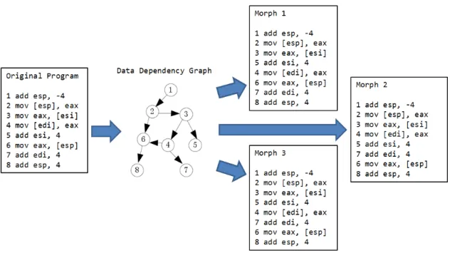
2.3.3 Instruction Transposition

Instruction Transposition takes the idea behind Subroutine Permutation and applies it at the basic block level. Basic blocks are sets of instructions that have one entry point and one exit point [15], all jumps must be contained within the set of instructions to be considered a basic block.

A Data-Dependency-Graph (DDG) can be created which represents the depen-dencies of each instruction in the basic block. Each reordering of branches creates a permutation of morphed output.

Figure 4 describes converting a DDG for an example basic block into some pos-sible morphed outputs. In the example, we can see that the path to instruction 5 can

Figure 4. Instruction Transposition

happen before instruction 4 is executed, the opposite is also true. Other permutations are also possible as seen in the diagram.

CHAPTER 3 LLVM

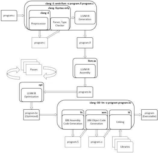
The Low Level Virtual Machine (LLVM) software is a compiler framework de-signed to reduce compiler code duplication across languages and architectures. It splits the functions of a compiler into a set of modular compiler components such that the core components can be shared and reused across different compilation schemes. This design is beneficial since it allows future work and optimization to be done in components that have multiple use-cases which can potentially improve code gener-ation for any language and architecture. LLVM uses these components to convert arbitrary high-level language code, such as C or C++, into an intermediate repre-sentation (IR). IR lies somewhere in-between the complexity of assembly and the simplicity of high-level languages. A diagram of LLVM is shown in Figure 5.

3.1 LLVM Intermediate Representation (IR)

LLVM IR provides type safety, low-level operations, and the capability of repre-senting ‘all’ high-level languages cleanly and is used throughout all phases of LLVM compilation strategy [16]. LLVM makes creation of new languages and syntax less cumbersome since compiler developers need only write code to convert new language grammar into LLVM IR. Subsequently, adding architectures is easier since developers need only write code to assemble LLVM IR into the architectures instruction code.

IR closely resembles assembly code, with the smallest unit of execution being labeled as an Instruction [17]. A sample of Human Readable IR Bytecode is provided in Figure 6.

3.2 LLVM Program Structure

Programs in LLVM are represented in a hierarchical container structure. The outermost representation, the Module [18], represents the entire program [19]. Mod-ules contain Function [20] objects, representing functions in the program. Functions contain BasicBlock [21] objects, which represent Basic Blocks. Basic Blocks contain Instruction [17] objects, which represent LLVM instructions in code. There is a cor-responding Instruction implementation for all IR byte code instructions. The LLVM container structure is shown visually in Figure 7.

3.3 LLVM Passes

To facilitate processing of LLVM IR bytecode, LLVM uses a data structure called a “Pass”, which are typically split up into three different types [22]; Analysis,

Trans-1 d e f i n e i32 @ m a i n () #0 { 2 e n t r y : 3 % r e t v a l = a l l o c a i32, a l i g n 4 4 %i = a l l o c a i32, a l i g n 4 5 % s t r = a l l o c a [13 x i8] , a l i g n 1 6 s t o r e i32 0 , i32* % r e t v a l 7 %0 = b i t c a s t [13 x i8]* % s t r to i8* 8 c a l l v o i d @ l l v m . m e m c p y . p 0 i 8 . p 0 i 8 .i64(i8* %0 , i8* g e t e l e m e n t p t r ← -i n b o u n d s ( [ 1 3 x i8]* @ m a i n . str , i32 0 , i32 0) , i64 13 , i32 1 ,←

-i1 f a l s e) 9 s t o r e i32 0 , i32* %i , a l i g n 4 10 br l a b e l % f o r . c o n d 11 12 for . c o n d : ; p r e d s = % f o r .← -inc , % e n t r y 13 %1 = l o a d i32* %i , a l i g n 4 14 % c o n v = s e x t i32 %1 to i64 15 % a r r a y d e c a y = g e t e l e m e n t p t r i n b o u n d s [13 x i8]* %str , i32 0 , i32 ← -0 16 % c a l l = c a l l i64 @ s t r l e n (i8* % a r r a y d e c a y ) #4 17 % c m p = i c m p ult i64 %conv , % c a l l

18 br i1 %cmp , l a b e l % f o r . body , l a b e l % f o r . end 19 20 for . b o d y : ; p r e d s = % f o r .← -c o n d 21 %2 = l o a d i32* %i , a l i g n 4 22 % i d x p r o m = s e x t i32 %2 to i64 23 % a r r a y i d x = g e t e l e m e n t p t r i n b o u n d s [13 x i8]* %str , i32 0 , i64 ← -% i d x p r o m 24 %3 = l o a d i8* % a r r a y i d x , a l i g n 1 25 % c o n v 2 = s e x t i8 %3 to i32 26 % c a l l 3 = c a l l i32 (i8* , . . . ) * @ p r i n t f (i8* g e t e l e m e n t p t r i n b o u n d s ←

-([3 x i8]* @ . str , i32 0 , i32 0) , i32 % c o n v 2 )

27 br l a b e l % f o r . inc 28 29 for . inc : ; p r e d s = % f o r .← -b o d y 30 %4 = l o a d i32* %i , a l i g n 4 31 % i n c = add nsw i32 %4 , 1

32 s t o r e i32 %inc , i32* %i , a l i g n 4 33 br l a b e l % f o r . c o n d 34 35 for . end : ; p r e d s = % f o r .← -c o n d 36 ret i32 0 37 }

Figure 7. LLVM Container Objects [3]

in some way, and may make use of information created from a prior Analysis pass. Utility passes are extra passes that don’t fit the Analysis/Transform model.

Passes can be written to function at different levels of the LLVM program struc-ture. A ModulePass is applied to the program Module. A FunctionPass is applied to the program Functions. A BasicBlockPass is applied to program BasicBlocks. Figure 8 describes program flow, applying Passes during LLVM execution.

Figure 8. LLVM High-Level Program Flow [3]

3.4 LLVM Toolchain

LLVM consists of many independent tools that collectively accomplish program compilation and assembly. Users chain these tools together to perform the desired functions. Tool use is performed within a command-line environment. Tools are executed on a variety of files, described by their extensions as follows:

• Human Readable IR Bytecode - “.ll”

• Binary IR Bytecode - “.bc”

• Architecture Specific Assembly - “.s”

Figure 9 displays LLVM tool flow, showing file transition during the multi-step compilation process. Tools are described in the following subsections. Many of the tools can also be applied by running clang (see 3.4.1).

3.4.1 clang

“Clang” is the C/C++ front-end for the LLVM project, it provides a gcc[23] compatible means to compile C/C++ code into various forms. These forms include pre-optimization LLVM IR bytecode, post-optimization LLVM IR bytecode, and na-tive machine code [24]. As a GCC-compatible compiler, clang integrates with the other tools in the LLVM tool suite to create fully compiled and linked executable programs from source code. When using the -emit-llvm option, clang will output Binary IR bytecode (.bc) if the output file has extension .bc, or a Human Readable IR bytecode (.ll) file if the output file has extension .ll.

3.4.2 llvm-as

The LLVM assembler, “llvm-as”, reads files containing human readable IR byte-code (.ll) and translates them into files containing Binary IR bytebyte-code (.bc) [25]. This tool is used to convert the output of llvm-dis or clang into Binary IR bytecode.

3.4.3 opt

The LLVM optimizer,“opt”, reads Binary IR bytecode and applies LLVM passes, outputting the product of those passes [26].

3.4.4 llvm-dis

The LLVM disassembler, “llvm-dis”, takes Binary IR bytecode and “converts it into human-readable LLVM assembly language” [27]. For this project, the primary use of this program is to inspect code.

3.4.5 llc

The LLVM static compiler, “llc”, takes Binary IR bytecode and compiles it “into assembly language for a specified architecture” [28].

3.5 Discussion

In summary, LLVM is a capable toolkit that provides a highly modular and ex-tensible code modification and analysis platform. The C++ Application Programmer Interface (API) is well documented [29], and there is a wealth of information available from other sources. The toolsuite includes a mechanism to inspect modifications us-ing Human Readable IR bytecode, providus-ing a means of verification and validation. These characteristics make LLVM a good candidate for creation of a morphing engine in the form of an LLVM Pass.

CHAPTER 4 Similarity Detection

4.1 Signature Detection

Signature-based detection uses a unique string of bits within a program to de-termine if that program is the same as another. Nearly all consumer-grade virus scanning software uses signature-based detection.

4.2 Hidden Markov Model (HMM)

A. A. Markov developed the idea of a “Markov Process” in 1907 [30]. A Markov process consists of a set of states and probabilities that describe the transition between those states, often represented by a state transition matrix, shown in Figure 11. Hidden Markov Models (HMM) are useful for understanding systems that can be represented with a Markov process, where the states of the process are not directly observable. A HMM is trained to generate a state transition matrix using observable states thought to be dependent in some way on the unobservable states of the hidden Markov process.

Figure 10 visually describes an HMM, where a set of hidden state transition probabilities (A) determines the hidden state transitions occurring in the hidden state sequence (X). Observations (Ot) influence the observation probability matrix (B) at hidden state (Xt).

sequence X occurring given observation statesO.

Figure 10. Hidden Markov Model [1] T = length of the observation sequence

N = number of states in the model

M = number of observation symbols

Q = {q0,q1, ...,qN−1} = distinct states of the Markov process V = {0, 1, ...,M−1} = set of possible observations

A = state transition probability matrix ={aij}, N ×N B = observation probability matrix ={bj(k)}, N×M

π = initial state distribution, 1×N

O = (O0,O1, ...,OT−1) = observation sequence X = (X0,X1, ...,XT−1) = hidden state sequence

λ = (A,B,π) = hidden markov model Table 1. HMM Notation [1]

aij =P(state qj at t+ 1 | state qi att) (1)

bj(k) = P(observation k at t | state qj att) (2)

P(X,O) = πx0bx0(O0)ax0,x1bx1(O1). . . axT−2,xT−1bxT−1(OT−1) (3)

HMM’s can be used to solve 3 different problems [1]:

1. Given a model and a sequence of observations, we can determine the likelihood of the observed sequence, P(O|λ) (see 4.2.2.1).

2. Given a model and a sequence of observations, we can find the optimal state sequence of the underlying Markov process, XOpt=f(O,λ) (see 4.2.2.2). 3. Given a sequence of observations, and dimensions N and M, we can generate a

model that maximizes the probability of the observed sequence (see 4.2.2.3).

4.2.1 HMM Example A= H C H 0.7 0.3 C 0.4 0.6

Figure 11. State Transition Probability Matrix [1]

M. Stamp developed a straightforward example to describe HMMs [1]. In this example, the objective is to determine if in the years before recorded history, those years were hot or cold, dependent on the sizes of tree rings, taken from trees that were living at the time. In this case, there is a Markov Chain with two states, Hot and Cold, which were historically unrecorded by humans. However a correlation is discovered between the sizes of tree rings and the temperature of the climate. We have a set of observable states, the values of which depend on unobservable states, an ideal case for an HMM. In this particular case, we can generate a state transition matrix using recorded data, let’s assume that the state transition matrix for this problem contains the data in Figure 11. We should also assume that the correlation between temperature and tree ring sizes is provided by Figure 12, and the initial state distribution is denoted by Figure 13.

B = S M L H 0.1 0.4 0.5 C 0.7 0.2 0.1

Figure 12. Observation Probability Matrix [1]

π =

H C

0.6 0.4

Figure 13. Initial State Distribution [1]

tions of sequences. The computed values are in Table 2. Column three of Table 2 provides normalized probabilities such that all rows sum to 1.

O = (S, M, S, L)

Figure 14. Example Observation Sequence [1]

state probability normalized probability HHHH .000412 .042787 HHHC .000035 .003635 HHCH .000706 .073320 HHCC .000212 .022017 HCHH .000050 .005193 HCHC .000004 .000415 HCCH .000302 .031364 HCCC .000091 .009451 CHHH .001098 .114031 CHHC .000094 .009762 CHCH .001882 .195451 CHCC .000564 .058573 CCHH .000470 .048811 CCHC .000040 .004154 CCCH .002822 .293073 CCCC .000847 .087963

Table 2. State sequence probabilities [1]

From Table 2 we can see that the most likely state sequence isCCCH. However, HMM’s allow us to find the sequence that maximizes the expected number of correct

states, computed by summing the probabilities for a given state at each position in the sequence. For example, as shown in Table 3, the HMM probability that the second state is equal toH is 0.519576. Thus, the optimal HMM-based sequence is CHCH.

element 0 1 2 3 P(H) 0.188182 0.519576 0.228788 0.804029 P(C) 0.811818 0.480424 0.771212 0.195971 Table 3. HMM Probabilities [1] 4.2.2 HMM Training

4.2.2.1 Solving 1: Forward Algorithm

To find P(O|λ), the forward algorithm, or α-pass, is used [1]. The probability of the partial observation up to time t, where the underlying Markov process is in state qt at time t [1], is shown in Equation 4. Computing the values of αt(i) using Equations 5 and 6 we can determine theαt(i) values for alltup toT−1. After which we can determine P(O|λ) using Equation 7.

αt(i) = P(O0,O1, ...,Ot,xt=qi | λ), for {t|0≤t < T}and {i|0≤i < N} (4) α0(i) =πibi(O0), for{i|0≤i < N} (5) αt(i) = "_N−1 X j=0 αt−1(j)aji # bi(Ot), for{t|1≤t < T} and {i|0≤i < N} (6) P(O|λ) = N−1 X i=0 αT−1(i) (7)

4.2.2.2 Solving 2: Backward Algorithm

To find XOpt, we can use the backward algorithm, or β-pass, which measures the relevant probability after time t. Using the data from the α-pass, we compute the β

values using Equations 9 and 10. Since the αt(i) represents probability leading up to

tandβt(i) represents probability following t[1], we can deduce that the most optimal state at timetis the state qi when these probabilities are highest, shown in Equation 13. βt(i) = P(Ot+1,Ot+2, ...,OT−1,xt =qi | λ), for {t|0≤t < T} and {i|0≤i < N} (8) βT−1(i) = 1, for {i|0≤i < N} (9) βt(i) = N−1 X j=0 aijbj(Ot+1)βt+1(j), for {t|T −2≥t ≥0}and {i|0≤i < N} (10) γt(i) = P(xt =qi|O,λ), for{t|0≤t < T} and {i|0≤i < N} (11) γt(i) = αt(i)βt(i) P(O|λ) (12)

XOpt(t) =qi for iwhen γt(i) = max

0≤i<Nγt(i) (13)

4.2.2.3 Solving 3: Model Building

We can train a model from observations using a hill-climb process. First we initialize λ = (A,B,π) using a best guess, or in near-uniform fashion such that

πi ≈ 1/N, aij ≈ 1/N, and bj(k) ≈ 1/M, while maintaining row-stochastic nature. Then we computeαt(i) (Equations 5, 6),βt(i) (Equations 9, 10), γt(i) (Equation 12), and γt(i,j) (Equation 15). We can then estimate the model using Equations 16, 17,

and 18. We hill climb this process through repetition, until P(O|λ) stops increasing. γt(i,j) =P(xt=qi,xt+1 =qj | O,λ), for {t|0≤t < T −1}and {i|0≤i,j < N} (14) γt(i,j) = αt(i)aijbj(Ot+1)βt+1(j) P(O|λ) (15) πi =γ0(i), for{i|0≤i < N} (16) aij = T−2 X t=0 γt(i,j) , _T−2 X t=0 γt (17) bj(k) = T−1 X t=0 Ot=k γt(j) , _T−1 X t=0 γt(j) (18) 4.2.3 HMM Use Cases

Hidden Markov Model (HMM) based detection uses a trained HMM to deter-mine if a program is similar enough to another program to be considered functionally equivalent. Research has shown that HMMs can be used to successfully detect meta-morphic viruses [7, 8, 12, 14], and are often used in pattern recognition applications, such as speech [31] and handwriting [32] recognition, and bioinformatics [33].

CHAPTER 5

Objective, Design, and Implementation

5.1 Introduction

The primary objective of this research is to perform code morphing such that the degree to which a morphing strategy is applied, is configured at run time. LLVM is an ideal tool to use to accomplish this, given the modularity of the toolchain.

5.2 Implementation

5.2.1 LLVM BasicBlockPass

Since the objective is to morph code, a transform pass is an ideal candidate. Morphing code requires adjustments at the Instruction level, and LLVM BasicBlocks contain Instructions, so an LLVM BasicBlockPass is one way to accomplish our ob-jective. A BasicBlockPass, “MorphingBasicBlockPass”, was developed in C++.

5.2.1.1 Features

Command line options are listed in Table 4. An example of execution is shown in Figure 15, where the degree for each strategy is set to a value of 30.

Option Description Input

add-degree The probability addition is applied 0-INT MAX

sub-degree The probability substitution is attempted 0-100 trs-degree The probability transposition is attempted 0-100 Note: Probabilities are evaluated for each original Instruction

opt -load MorphingBasicBlockPass.so -MorphingBasicBlockPass -add-degree 30 -sub-degree 30 -trs-degree 30 < F ILE.bc >

M ORP HED F ILE.bc

Figure 15. Morphing Pass Command Line Example

5.2.1.2 Morphing

Morphing degree is defined by user input. For each BasicBlock, an iteration is performed over the Instruction objects. With each iteration, a random distribution of 1 to 100 is used to select a random number for comparison with the given morphing strategy degree. If the random number is less than or equal to the degree, this is considered a “hit” and the morphing strategy is attempted using that Instruction. Multiple strategies can be applied to the same instruction if more than one strategy has a “hit”. In the case of addition, a multiplier effect is applied if the add-degree is greater than 100, this guarantees that for each multiple of 100, an instruction is added.

5.2.1.2.1 Addition

The code addition strategy adds dead code to the program. When a hit occurs, a randomly selected Instruction object is created and inserted into the Instruction object list in the BasicBlock, after the current Instruction object in iteration. A vector of enumerations, representing instructions, is used with a randomly selected index, bounded by the vector size, to determine the instruction to add. Possible instructions added are shown in Table 5.

To mitigate constant folding, where the compiler pre-computes constant values at compile time and optimizes them out, at the start of each BasicBlock, a 64-bit integer

Enumeration Returns LLVM Instruction x86 Output

BINARY OP ADD int64 add add

BINARY OP SUB int64 sub sub

BINARY OP MUL int64 mul mul

BINARY OP DIV int64 div div

BINARY OP REM int64 urem div

BINARY OP SHL int64 shl shl

BINARY OP LSHR int64 lshr shr

BINARY OP ASHR int64 ashr sar

BINARY OP AND int64 and and

BINARY OP OR int64 or or

BINARY OP XOR int64 xor xor

ICMP TRUE int1 icmp true cmp

ICMP FALSE int1 icmp false cmp

BINARY OP FADD float fadd addsd

BINARY OP FSUB float fsub subsd

BINARY OP FMUL float fmul mulsd

BINARY OP FDIV float fdiv divsd

BINARY OP FREM float frem divsd

FCMP TRUE int1 fcmp true cmp

FCMP FALSE int1 fcmp false cmp

Table 5. Code Addition Mapping

to the previously added dead code instruction. At the end of the BasicBlock, the final value is written back to memory, this ensures that the compiler does not optimize-out the added code. In addition, as each dead code instruction is added, two vectors store pointers to previously added dead code instructions, depending on the type of dead code instruction to be added, an Integer or Floating Point value is randomly selected from these vectors to be used as one of the instruction operands. This creates a dependency between the added Instruction, the preceding dead code instruction, and a randomly selected previously added instruction, which further mitigates compiler optimization. LLVM is type aware, and will not allow operands of incorrect type to be passed into Instructions. When the Instruction to be chained as an operand is of the wrong type, a CastInst Instruction is added to convert the type.

Figure 16 displays a snippet of pre-morphed Human Readable IR bytecode taken from a simple hello world program, performing the conditional part of a for loop. Fig-ure 17 contains a snippet of morphed Human Readable IR bytecode. The parameters of the morphing are -add-degree=100 -sub-degree=0.

1 for . c o n d : ; p r e d s = % f o r .← -inc , % e n t r y 2 %1 = l o a d i32* %i , a l i g n 4 3 % c o n v = s e x t i32 %1 to i64 4 % a r r a y d e c a y = g e t e l e m e n t p t r i n b o u n d s [13 x i8]* %str , i32 0 , i32 ← -0 5 % c a l l = c a l l i64 @ s t r l e n (i8* % a r r a y d e c a y ) #4 6 % c m p = i c m p ult i64 %conv , % c a l l

7 br i1 %cmp , l a b e l % f o r . body , l a b e l % f o r . end

Figure 16. Pre-Morphed Human Readable IR Bytecode

1 for . c o n d : ; p r e d s = % f o r .← -inc , % e n t r y 2 %16 = a l l o c a i64 3 %17 = l o a d v o l a t i l e i64* %16 4 %18 = a s h r i64 %17 , 47 5 %19 = l o a d i32* %i , a l i g n 4 6 %20 = s i t o f p i64 %18 to d o u b l e 7 %21 = f a d d d o u b l e 0 x 7 F E 9 8 2 0 F C 1 E 8 4 7 0 C , %20 8 % c o n v = s e x t i32 %19 to i64 9 %22 = f p t o s i d o u b l e %21 to i64 10 %23 = a s h r i64 %22 , 46 11 % a r r a y d e c a y = g e t e l e m e n t p t r i n b o u n d s [13 x i8]* %str , i32 0 , i32 ← -0 12 %24 = s i t o f p i64 %23 to d o u b l e 13 %25 = f c m p f a l s e d o u b l e 0 x 7 F C 3 8 5 A 2 4 3 6 8 2 4 7 7 , %24 14 %26 = z e x t i1 %25 to i64 15 % c a l l = c a l l i64 @ s t r l e n (i8* % a r r a y d e c a y ) #4 16 %27 = l s h r i64 %26 , 39 17 s t o r e v o l a t i l e i64 %27 , i64* %16

18 % c m p = i c m p ult i64 %conv , % c a l l

19 br i1 %cmp , l a b e l % f o r . body , l a b e l % f o r . end

tions. When a hit occurs, the current instruction is evaluated to determine if it is suitable for substitution, if not, the substitution operation is aborted. As shown in Table 6; an “add” operation is replaced with a negate and “sub”, a “sub” operation is replaced with a negate and “add”. LLVM does not have an IR representation for “neg”, and instead uses subtraction against zero [16].

Input (LLVM) → Output (LLVM) → Output (x86)

O = add x y → O

0 _{= sub 0 x}

O = sub y O0 → subsub

O = fadd x y → O

0 _{= fsub 0 x}

O = fsub y O0 → subsdsubsd

O = sub x y → O

0 _{= sub 0 x}

O = add O0 y → subadd

O = fsub x y →

O0 = fsub 0 x

O = fadd O0 y → subsdaddsd Table 6. Code Substitution Mapping

5.2.1.2.3 Transposition

Transposition uses the DependenceAnalysis [34] process to determine instruction dependencies. In testing, this feature frequently returned that instructions were de-pendent on previous instructions, and in some cases where dependencies were not detected, inspection of the code showed that a dependence did indeed exist. Alter-native mechanisms to leverage LLVM for dependence analysis were searched for, but none were found. As a result, the user-input to configure transposition degree, and the strategy activation code exists but the morphing strategy is not implemented.

5.2.1.3 Validation

Validation was performed by executing the full toolchain on pre-morphed and morphed code. Comparisons were performed at both the LLVM IR Bytecode phase (see Figures 16, 17), and at the post-assembled phase, by performing opcode

extrac-tion (see 5.2.2). Figure 18 contains a secextrac-tion of opcodes extracted from a “hello world” test program that was not morphed. Figure 19 contains the corresponding section of opcodes extracted from a morphed variant of the “hello world” test program listed above. The parameters of the morphing were-add-degree=30 -sub-degree=0. The following LLVM instructions were added to this section as part of the morphing, line numbers of the result listed in parenthesis: icmp false (ln. 7), lshr (ln. 12), and lshr (ln. 20). 1 nop D W O R D PTR [rax] 2 p u s h rbp 3 mov rbp,rsp 4 sub rsp,0 x30 5 mov D W O R D PTR [rbp-0 x4 ] ,0 x0 6 mov rax,Q W O R D PTR ds :0 x 4 0 0 6 8 0 7 mov Q W O R D PTR [rbp-0 x15 ] ,rax 8 mov ecx,D W O R D PTR ds :0 x 4 0 0 6 8 8 9 mov D W O R D PTR [rbp-0 xd ] ,ecx 10 mov dl,B Y T E PTR ds :0 x 4 0 0 6 8 c 11 mov B Y T E PTR [rbp-0 x9 ] ,dl 12 mov D W O R D PTR [rbp-0 x8 ] ,0 x0 13 lea rdi,[rbp-0 x15 ] 14 m o v s x d rax,D W O R D PTR [rbp-0 x8 ] 15 mov Q W O R D PTR [rbp-0 x20 ] ,rax 16 c a l l 4 0 0 4 3 0 < s t r l e n @ p l t > 17 mov rdi,Q W O R D PTR [rbp-0 x20 ] 18 cmp rdi,rax 19 jae 4 0 0 5 e1 < m a i n +0 x81 > 20 m o v a b s rdi,0 x 4 0 0 6 8 d 21 m o v s x d rax,D W O R D PTR [rbp-0 x8 ] 22 m o v s x esi,B Y T E PTR [rbp+rax*1 -0 x15 ] 23 mov al,0 x0

Figure 18. Pre-Morphed Extracted Opcodes

5.2.2 Opcode Extraction

1 nop D W O R D PTR [rax] 2 p u s h rbp 3 mov rbp,rsp 4 sub rsp,0 x50 5 m o v a b s rax,0 x 7 c 2 8 5 2 d 3 e 7 0 1 4 b 1 c 6 mov rcx,Q W O R D PTR [rbp-0 x8 ] 7 cmp rax,rcx 8 s e t n e dl 9 and dl,0 x1 10 m o v z x esi,dl

11 mov eax,esi 12 shr rax,0 x28 13 mov D W O R D PTR [rbp-0 xc ] ,0 x0 14 mov rcx,Q W O R D PTR ds :0 x 4 0 0 7 b 0 15 mov Q W O R D PTR [rbp-0 x1d ] ,rcx 16 mov esi,D W O R D PTR ds :0 x 4 0 0 7 b 8 17 mov D W O R D PTR [rbp-0 x15 ] ,esi 18 mov dl,B Y T E PTR ds :0 x 4 0 0 7 b c 19 mov B Y T E PTR [rbp-0 x11 ] ,dl 20 shr rax,0 x1f 21 mov Q W O R D PTR [rbp-0 x8 ] ,rax 22 mov D W O R D PTR [rbp-0 x10 ] ,0 x0 23 lea rdi,[rbp-0 x1d ] 24 mov rax,rsp 25 add rax,0 x f f f f f f f f f f f f f f f 0 26 mov rsp,rax

27 mov rax,Q W O R D PTR [rax]

28 m o v s x d rcx,D W O R D PTR [rbp-0 x10 ] 29 mov Q W O R D PTR [rbp-0 x28 ] ,rcx 30 mov Q W O R D PTR [rbp-0 x30 ] ,rax 31 c a l l 4 0 0 4 f0 < s t r l e n @ p l t > 32 mov rcx,Q W O R D PTR [rbp-0 x28 ] 33 cmp rcx,rax 34 jae 4 0 0 6 fd < m a i n +0 xdd > 35 m o v a b s rdi,0 x 4 0 0 7 b d 36 mov rax,rsp 37 add rax,0 x f f f f f f f f f f f f f f f 0 38 mov rsp,rax

39 mov rax,Q W O R D PTR [rax]

40 m o v s x d rcx,D W O R D PTR [rbp-0 x10 ] 41 m o v s x esi,B Y T E PTR [rbp+rcx*1 -0 x1d ] 42 mov Q W O R D PTR [rbp-0 x38 ] ,rax

43 mov al,0 x0

Figure 19. Morphed Extracted Opcodes (add = 30, sub & trs = 0)

tool chosen for this research, is part of the Linux GNU binutils [35] package. Opcodes are extracted using the Intel standard assembly syntax [36], text output is parsed

using grep [37] and awk [38]. For similarity detection, opcodes go through a cleanup process, a simple program, “filteropcodes” was developed in C++. Filteropcodes compares each value of a potential opcode with a file containing 697 valid opcodes, taken as input, and filters out invalid entries, removing non-code data leftover from the initial parsing phase. The valid opcode mnemonics were retrieved from an XML file [39] using an XSL stylesheet. An example command-line execution of the opcode extraction process is shown in Figure 20.

o b j d u m p - M x86_64 , intel - m n e m o n i c - - no - show - raw - i n s n - S $B I N A R Y | g r e p ’ [0 -9 a - zA - Z ]*\: ’ | awk ’!($1 = " " ) ’ | awk ’{ p r i n t $1 } ’ >

$P R E F I L T E R E D _ O P C O D E S

f i l t e r o p c o d e s $V A L I D _ I N S T R U C T I O N S $P R E F I L T E R E D _ O P C O D E S

$F I L T E R E D _ O P C O D E S

Figure 20. Objdump Execution Example

5.2.3 Similarity Detector (HMM)

An HMM implementation was written in C++. Two programs were developed, a HMM building program “hmm” that trains an HMM from input data, and an HMM scoring program “hmmscore”, that uses a model to score input data. The programs leverage an “OTHER” observation, that captures any input that is not present in the set of observation states in the model.

5.2.3.1 Observation State Selection

Since computational demand increases as the HMM matrices increase in size, the set of Observation states was bounded at a size of 26. To determine the most useful instructions to include, objdump was executed on all morphed variants of the

5.2.3.2 Validation

The “hmm” program was validated by performing the “not-so-simple example” in [1], using the “Brown Corpus” and an HMM with two hidden states to separate between vowels and consonants in English language. Program output that has the expected result is shown in Figure 21.

CHAPTER 6 Experiments

6.1 Dataset

Data was generated from GNU coreutils [40], a suite of Linux commands. The largest command, “ls”, was selected as a program to perform morphing on. The other commands were used as the benign data set. The benign data was compiled using optimization level 2 (-O2).

6.1.1 Training Data

Training data was generated using an Add Degree of 1, the binaries were compiled using clang with a compiler optimization of 0 (-O0). 50 variant files were generated, with an average of 2.06% code morphing. The variant files were concatenated to-gether, and the concatenated file was used as the input for HMM training. The model is shown in Table 7.

6.1.2 Test Data

Test data was generated using varying add-degree values: 25, 50, 100, 200, 400, 800, 1600, and 3200. This non-linear approach was chosen because a non-linear rate of change in scoring was observed during initial trial and error. The test data binaries were compiled using clang with a compiler optimization of 0 (-O0). 50 files were generated for each add-degree.

π 0.0000000000000000000 1.0000000000000000000 A 0.8637300479230411998 0.1362699520770013772 0.0860074392855465775 0.9139925607138835728 B OTHER 0.0699936581903331939 0.0082915228540217534 add 0.0014958661667065841 0.0727099056793662213 and 0.0189049567728136435 0.0127566754956268645 call 0.0323666911830608126 0.0693702185449694003 cmp 0.1366788506795023339 0.0000000000000000000 ja 0.0027361093554276713 0.0023912945970399435 jae 0.0139133354969235481 0.0000000000000000000 je 0.0701424017120766408 0.0000000000000000000 jge 0.0066208286157774122 0.0000000000000000000 jmp 0.1332991576448592508 0.0340140401570356993 jne 0.0678759673366467475 0.0000000000000000000 lea 0.0006118131491648823 0.0108553295640027355 mov 0.3259771411192445290 0.6273424358217389862 movss 0.0113590390077642038 0.0000000000000000000 movsx 0.0148211450127546766 0.0015781868146700286 movsxd 0.0028243810806406516 0.0065603714315576973 movzx 0.0061572871657375816 0.0089080851421619849 nop 0.0000000000000000000 0.0159047351172595733 or 0.0027514345427740879 0.0017130199723750384 pop 0.0000000000000000000 0.0258077976653301178 push 0.0107248596738458608 0.0262407658962855901 retn 0.0000000000000000000 0.0244669598178846558 shl 0.0000000000000000000 0.0036337069036462360 sub 0.0070663228602007655 0.0350336106545953083 test 0.0451310221905035919 0.0000000000000000000 xor 0.0185477310435632516 0.0124213378703803973

Table 7. Trained HMM Model

6.2 Experimental Method

Using the model generated from the training data, the “benign” coreutils data, and the morphed test data, HMM scores were computed. Results are in the following section.

6.3 Results

Figure 22 displays HMM scores for each data point across the different morphing degrees. Blue triangles reflect the Training Data, green triangles reflect the Benign Data, and the data points of various shapes following a gradient from black to red

represent the morphed variants. We can see that around add-degree of 400, the morphed code becomes indistinguishable from the benign data.

0 5 10 15 20 25 30 35 40 45 50 −3 −2.8 −2.6 −2.4 −2.2 −2 −1.8 Number of Files HMM Score

T raining Benign M orph 25 M orph50 M orph100

M orph200 M orph 400 M orph800 M orph1600 M orph 3200 Figure 22. HMM Score Vs. Morphing Degree

Table 8 provides the percentage of dead code added to a file for each morphing degree, calculated by subtracting the size of the original executable from the size of the morphed variant, and dividing the result by the size of the original executable. An add-degree of 400 causes a 433.38% increase in executable size.

Figure 23 displays Receiver Operating Characteristic (ROC) curves for Add De-gree’s 200, 400, 800, and 1600. We can see from the charts that the HMM begins to

Add Degree Code Added (%) 25 41.86 50 84.36 100 191.54 200 285.14 400 433.38 800 671.82 1600 1,051.45 3200 1,672.49

Table 8. Add Degree vs. Code Added

0 0.1 0.2 0.3 0.4 0.5 0.6 0.7 0.8 0.9 1 0 0.1 0.2 0.3 0.4 0.5 0.6 0.7 0.8 0.9 1

False Positive Rate

T rue P ositiv e Rate Add Degree 200 0 0.1 0.2 0.3 0.4 0.5 0.6 0.7 0.8 0.9 1 0 0.1 0.2 0.3 0.4 0.5 0.6 0.7 0.8 0.9 1

False Positive Rate

T rue P ositiv e Rate Add Degree 400 0 0.1 0.2 0.3 0.4 0.5 0.6 0.7 0.8 0.9 1 0 0.1 0.2 0.3 0.4 0.5 0.6 0.7 0.8 0.9 1

False Positive Rate

T rue P ositiv e Rate Add Degree 800 0 0.1 0.2 0.3 0.4 0.5 0.6 0.7 0.8 0.9 1 0 0.1 0.2 0.3 0.4 0.5 0.6 0.7 0.8 0.9 1

False Positive Rate

T rue P ositiv e Rate Add Degree 1600

Figure 23. ROC Curves for Add Degrees 200, 400, 800, and 1600

The Area Under the Curve (AUC) for the data is shown in Table 9, we can see that the number of false positives does not increase between 1600 and 3200 Add Degree, which is suggestive that the HMM score plateaus at very high levels of mor-phing. This is expected, since the HMM score is a value normalized by the number of opcodes in the program.

Add Degree AUC 25 1.000 50 1.000 100 1.000 200 1.000 400 0.8364 800 0.5912 1600 0.5400 3200 0.5400

Table 9. ROC AUC Statistics for Add Strategy

Unexpectedly, the Add Degree 25 and Add Degree 50 sets appear to score better than the original training data. Reviewing Figure 22, we can see the non-linear fashion in which scores improve relative to code added. At very high Add Degrees, the score improves very little, and it takes a significant increase, 433.38%, in program size to evade HMM detection. Additional datasets were evaluated and are provided in Appendix A. These include scoring optimized morphed variants using a model trained with non-optimized data (see A.1), scoring non-optimized variants using a model trained with optimized data (see A.2), and scoring optimized variants using a model trained with optimized data (see A.3).

In summary, the HMM is highly effective at determining the similarity of the morphed program when compiler optimization 0 is used during compilation. The HMM was fully successful in differentiating the benign data from morphed variants up to Add Degree 200. At Add Degree 400 the HMM started to provide similar scores to that of the benign data.

CHAPTER 7 Conclusion

In this project, we investigated a new approach using the LLVM Pass API to generate highly random morphed variants of software. Dead code was added at vari-ous degrees and a model was trained using an HMM to determine both the strength of this morphing approach, and the strength of the HMM. Leveraging a custom de-veloped BasicBlocksPass, we intertwined dead code within the very low levels of a program in an attempt to defeat compiler optimization, such that the dead code was preserved.

We discovered that HMM’s are an effective detection mechanism in regards to software that is morphed using this approach. We also discovered that at very high morphing rates, the HMM becomes less effective at properly classifying the origin of the morphed program. In the case tested, the HMM was capable of properly classifying the morphed program up until 433% of dead code was added.

There are many improvements that can be made to this code generator. These in-clude incorporating instruction transposition using LLVM’s Dependence Analysis ca-pability (an original goal of this project), adding new instruction substitution schemes, and increasing the precision of dead code insertion.

LIST OF REFERENCES

[1] M. Stamp, “A revealing introduction to hidden markov models,” 2015.

[2] “What is arc in ios.” 2015. [Online]. Available: https://iphonecodecenter. wordpress.com/2015/10/06/what-is-arc-in-ios/

[3] “Adrian sampson: Llvm for grad students.” [Online]. Available: https: //www.cs.cornell.edu/∼_{asampson/blog/llvm.html}

[4] M. Stamp,Information Security: Principles and Practice. Wiley, 2011. [5] P. Szor,The Art of Computer Virus Research and Defense. Pearson, 2005. [6] P. F. F. Perriot, P. Szor. “Striking similarities - win32/simile and metamorphic

virus code.” 2003. [Online]. Available: https://www.symantec.com/avcenter/ reference/striking.similarities.pdf

[7] S. Venkatachalam, “Detecting undetectable computer viruses,” Master’s thesis, Department of Computer Science, San Jose State University, 2010.

[8] W. Wong, “Analysis and detection of metamorphic computer viruses,” Master’s thesis, Department of Computer Science, San Jose State University, 2006. [9] D. Baysa, “Structural entropy and metamorphic malware,” Master’s thesis,

De-partment of Computer Science, San Jose State University, 2012.

[10] “Mpcgen v1.0.” 2013. [Online]. Available: http://www.textfiles.com/virus/ DOCUMENTATION/mpcgen.txt

[11] “Metamorphic permutating high-obfuscating reassembler.” 2013. [Online]. Available: http://dsr.segfault.es/stuff/website-mirrors/29A/29a-6/29a-6.602 [12] D. Lin, “Hunting for undetectable metamorphic viruses,” Master’s thesis,

De-partment of Computer Science, San Jose State University, 2009.

[13] Normalization towards Instruction Substitution Metamorphism Based on Stan-dard Instruction Set, 2007.

[14] T. Tamboli, “Metamorphic code generation from llvm ir bytecode,” Master’s thesis, Department of Computer Science, San Jose State University, 2013.

[16] “Llvm language reference manual.” 2017. [Online]. Available: http://llvm.org/ docs/LangRef.html

[17] “Llvm: llvm::instruction class reference.” 2017. [Online]. Available: http: //llvm.org/doxygen/classllvm 1 1Instruction.html

[18] “Llvm: llvm::module class reference.” 2017. [Online]. Available: http: //llvm.org/doxygen/classllvm 1 1Module.html

[19] “Llvm language reference manual.” 2017. [Online]. Available: https: //llvm.org/docs/LangRef.html#high-level-structure

[20] “Llvm: llvm::function class reference.” 2017. [Online]. Available: http: //llvm.org/doxygen/classllvm 1 1Function.html

[21] “Llvm: llvm::basicblock class reference.” 2017. [Online]. Available: http: //llvm.org/doxygen/classllvm 1 1BasicBlock.html

[22] “Llvm’s analysis and transform passes - llvm 6 documentation.” 2017. [Online]. Available: https://llvm.org/docs/Passes.html

[23] “Gcc, the gnu compiler collection - gnu project - free software foundation (fsf).” 2017. [Online]. Available: https://gcc.gnu.org/

[24] “Clang compiler user’s manual - clang 6 documentation.” 2017. [Online]. Avail-able: https://clang.llvm.org/docs/UsersManual.html#command-line-options [25] “llvm-as - llvm assembler - llvm 6 documentation.” 2017. [Online]. Available:

https://llvm.org/docs/CommandGuide/llvm-as.html

[26] “opt - llvm optimizer - llvm 6 documentation.” 2017. [Online]. Available: https://llvm.org/docs/CommandGuide/opt.html

[27] “llvm-dis - llvm disassembler - llvm 6 documentation.” 2017. [Online]. Available: https://llvm.org/docs/CommandGuide/llvm-dis.html

[28] “llc - llvm static compiler - llvm 6 documentation.” 2017. [Online]. Available: https://llvm.org/docs/CommandGuide/llc.html

[29] “Llvm programmer’s manual - llvm 6 documentation.” 2017. [Online]. Available: http://llvm.org/docs/ProgrammersManual.html

[30] “Introduction to probability.” 2017. [Online].

Avail-able: https://www.dartmouth.edu/∼_{chance/teaching aids/books articles/} probability book/amsbook.mac.pdf

[31] M. Gales and S. Young, “The application of hidden markov models in speech recognition,” in Foundations and Trends in Signal Processing, M. Gales and S. Young, Eds. Now Publishers, 2007, pp. 195–304.

[32] A. Kundu, “Handwritten word recognition using hidden markov model,” in Handbook of Character Recognition and Document Image Analysis, P. S. W. H. Bunke, Ed. World Scientific Publishing Company, 1997, ch. 6, pp. 157–182. [33] B. Yoon, “Hidden markov models and their applications in biological sequence analysis,” in Current Genomics. Bentham Science Publishers Ltd., 2008, pp. 402–415.

[34] “Llvm: llvm::dependenceanalysis class reference.” 2017. [Online]. Available: http://llvm.org/doxygen/classllvm 1 1DependenceAnalysis.html

[35] “Binutils - gnu project - free software foundation.” 2017. [Online]. Available: https://www.gnu.org/software/binutils/

[36] N. Matloff. “Introduction to linux intel assembly language.” 2002. [Online]. Available: http://heather.cs.ucdavis.edu/∼_{matloff/50/LinuxAssembly.html} [37] “Grep - gnu project - free software foundation.” 2017. [Online]. Available:

https://www.gnu.org/software/grep/

[38] “Gawk - gnu project - free software foundation.” 2017. [Online]. Available: https://www.gnu.org/software/gawk/

[39] “x86reference.xml.” 2017. [Online]. Available: http://ref.x86asm.net/ x86reference.xml

[40] “Coreutils - gnu project - free software foundation.” 2017. [Online]. Available: https://www.gnu.org/software/coreutils/coreutils.html

APPENDIX Additional Datasets

A.1 Dataset 2: O0 Training, O2 Morphed

0 5 10 15 20 25 30 35 40 45 50 −3 −2.8 −2.6 −2.4 −2.2 −2 Number of Files HMM Score

T raining Benign M orph25 M orph 50 M orph 100

M orph200 M orph 400 M orph 800 M orph 1600 M orph3200 Figure A.24. Dataset 2: HMM Score Vs. Morphing Degree

Add Degree Code Added (%) 25 -8.5 50 13.05 100 55.96 200 72.49 400 95.58 800 133.43 1600 193.29 3200 284.59

Table A.10. Dataset 2: Add Degree vs. Code Added

A.2 Dataset 3: O2 Training, O0 Morphed

0 5 10 15 20 25 30 35 40 45 50 −2.7 −2.6 −2.5 −2.4 −2.3 −2.2 −2.1 −2 Number of Files HMM Score

T raining Benign M orph25 M orph 50 M orph 100

M orph200 M orph 400 M orph 800 M orph 1600 M orph3200 Figure A.25. Dataset 3: HMM Score Vs. Morphing Degree

Add Degree Code Added (%) 25 114.63 50 178.38 100 339.34 200 479.93 400 703.07 800 1,058.79 1600 1,633.49 3200 2,582.34

Table A.11. Dataset 3: Add Degree vs. Code Added

A.3 Dataset 4: O2 Training, O2 Morphed

0 5 10 15 20 25 30 35 40 45 50 −2.7 −2.6 −2.5 −2.4 −2.3 −2.2 −2.1 Number of Files HMM Score

T raining Benign M orph25 M orph 50 M orph 100

M orph200 M orph 400 M orph 800 M orph 1600 M orph3200 Figure A.26. Dataset 4: HMM Score Vs. Morphing Degree

Add Degree Code Added (%) 25 37.65 50 69.95 100 135.35 200 159.44 400 193.83 800 251.00 1600 343.37 3200 481.42

Table A.12. Dataset 4: Add Degree vs. Code Added

A.4 Dataset 5: O2 Trained Model Investigation

Comparing the scores of the O2 training data and the scores of 1,931 benign files from/usr/binin a CentOS 7.4 Operating System, we can see that this model is not producing a very useful capability of differentiating morphed data from unmorphed data when compiler optimization is used. Figure A.27 displays the scores of the benign files against the training data. When using a model with Add Degree 30 for the training data, shown in Figure A.28, the scoring against the benign data is much better, though there are still many benign files that might be considered a match. When testing this higher degree model against the original Add Degree 1 training data, the HMM is unable to differentiate it from many benign programs in terms of similarity. This is a crude analysis, and doesn’t take into account the underlying functionality of these benign files, which may be similar enough in function to be considered a match.

0 5 10 15 20 25 30 35 40 45 50 −3 −2.8 −2.6 −2.4 −2.2 −2 −1.8 −1.6 Number of Files HMM Score T raining Benign

0 5 10 15 20 25 30 35 40 45 50 −3.4 −3.2 −3 −2.8 −2.6 −2.4 −2.2 −2 −1.8 Number of Files HMM Score

T raining (a30) Benign M orphed ls (a1)

Figure A.28. Dataset 5: Training Score (Model a30) Vs. /usr/bin Benign Files, a1-O2 morphed ls