Essays on firm dynamics

Beatriz Gonz´

alez L´

opez

In partial fulfillment of the requirements for the degree of

Doctor in Economics

Universidad Carlos III de Madrid

Advisor:

Andr´

es Erosa Etchebehere

First and foremost, I want to thank Andr´es, for so many things I do not know where to begin. Thank you for introducing me to macroeconomics and to research, for always pushing me to be my best self, for our endless discussions about research, for being kind and supportive, for being a guide and a friend. Thank you.

I am very thankful to Timothy Kehoe for his kind invitation to visit the University of Minnesota. I especially thank him and Manuel Amador for invaluable guidance and insights to improve my research. I am also grateful to Anmol Bandhari, Ellen McGrattan, Kyle Herkenhoff and Loukas Karabarbounis for helpful comments.

I would also like to thank the professors of the department of economics at UC3M, especially the macro group. Thank you Matthias for organizing the reading group (and the beers afterwards) and for always being available for us. I would also like to thank Emircan, Antonia, Luisa, Felix, Hern´an, Bel´en and Asier for their comments and help throughout my PhD. Special thanks to Arancha and Ang´elica, who have always done their best to support us in all the administrative related stuff.

It is still hard to believe that I am here writing down the acknowledgements of my dissertation, when the first day of the master feels like yesterday. I remember looking for flats around Getafe with my flatmates and classmates to be, Ana, Conchi and Ursula, with whom I have shared so many joys and sufferings, thank you very much for your friendship and for being there since the beginning. Of course, our cohort would not have been the same without Tom´as, Cris, Junji, Kai, Luis, Rui and Yuhao. Once I started the PhD, I have been lucky to have the best officemates: Mehdi, Alessandro, you were the reason why I was looking forward to come to the office; and of course Rui and Ismael, with whom I have shared so much. It was great to have Onursal, Javi, Michele, Michelangelo, Elizaveta, Mar´ıa and Sergio as PhD colleagues these years. I am especially grateful to have met some people that I am lucky enough to call my friends. Federico Curci, the official party organizer, whose positive attitude would spark joy to anyone near him; Federico Masera, my official PhD guide, one of the person with whom I disagree the most, but with whom I would share pretty much anything (I miss you so much!); Salvatore Lo Bello, his charisma and

partner, a great officemate and one of the best friends I could have asked for. During these years, I enjoyed practising crossfit at UC3M, an activity that helped me get through the rough moments of the PhD. With Tom´as, and all the participants of these classes, we have created a group of friends that hopefully will last for long after the PhD.

Of course, my stay in Minnesota would not have been the same without all the graduate students that, apart from helping me evolve as a researcher, made my stay full of unforget-table memories. Keyvan, my first contact with the Minnesota group; my officemates Salim, Luis and Fatih, and of course Ross and Guillaume; days at the gym, barbeques, house parties and what not with the guys (Agust´ın, Carlos, Fausto, Marcos, Carlo, Salom´on, Alex and the Arizona guys Alberto and Santi); cross-country skiing with Jarek, Vladimir and Diana; a party on a boat with los Sergios and Camila; the Spanish crew Joaqu´ın, Eugenia and Sergi; and of course lady’s nights with Emily, Sandra, Amy, Tobey, Mariajo and Leticia. Thank you all. I would also like to thank the Jensen family, to whom I will be eternally indebted.

Finally, I want to thank my family for always supporting me. I would like to thank especially my parents, Javier and Mar´ıa Jos´e, and my sister Elena, for their unconditional love and help when I needed it the most. And, of course, Daniel, thank you for always being there for me, you are my anchor, I could not have done this without you.

Chapter 1 of this thesis, the paper ‘Taxation and the Life Cycle of Firms’, is accepted for publication. It will appear in the Journal of Monetary Economics, Volume 105; August 2019.

This thesis has been possible thanks to the financial support of Fundaci´on La Caixa (ID 100010434), grant number LCF/BQ/ES15/10360005.

There is a growing interest among macroeconomists in incorporating explicit heterogeneity into macroeconomic models, allowing to bring in micro data to discipline them. In this way, we can understand how shocks or policies impact differently these heterogeneous agents and their macroeconomic implications, which sometimes might differ from those obtained using a representative agent model. My dissertation consists of two main chapters that attempt to understand the impact of changes in the economic environment, with a special focus on taxes, on heterogeneous firms’ investment and growth decision, the firm size distribution of firms, and ultimately their impact on macroeconomic aggregates.

In the first chapter, ‘Taxation and the Life Cycle of Firms’, co-authored with Andr´es Erosa, we extend theHopenhayn and Rogerson(1993) framework to understand how different forms of taxing capital income affect firms’ investment and financial policies over their life cycle. Relative to dividends and capital gains taxation, corporate income taxation slows down firm growth over the life cycle by reducing after-tax profits available for reinvesting. It also diminishes entry by negatively affecting the value of entrants relative to that of incumbent firms. After a tax reform eliminating the corporate income tax in a revenue neutral way, output and capital increase by 12% and 32%. The large response of firm entry is crucial for these results.

In the second chapter, ‘Macroeconomics, Firms Dynamics and IPOs’, I study how changes in the economic environment witnessed in the US in the last decades regarding taxes, access to credit and idiosyncratic productivity shock process impact firms’ choices. I argue these changes might impact differently privately held and publicly traded firms, having therefore implications for the endogenous decision to become public (IPO) and their macroeconomic consequences. I extend a model of firm dynamics with private and publicly traded firms, where I explicitly model the going public decision. Firms are born private, grow by reinvesting profits and/or borrowing, and can eventually do an IPO and become public. Being public, firms can access to costly equity financing, but have to pay an ongoing cost of operation. I calibrate the model to the US, and study how the observed changes in the last decades of taxes, equity issuance costs, the costs of being public, access to credit and

1990s contributes to the increase in share of public firms, and the changes in firms’ policies observed in the data, having a larger impact than changes in equity issuance costs. An increase in the cost of being public is at odds with the changes in selection into public and firms’ policies observed in the data during the 2000s, and so is an increase access to credit. Changes in the idiosyncratic shock process can reconcile some of the trends in behaviour and selection of publicly traded firms, and have important macroeconomic implications.

1 Taxation and the Life Cycle of Firms 1

1.1 Introduction . . . 1

1.2 A Simple Deterministic Model Economy . . . 5

1.2.1 The problem of a firm . . . 5

1.2.2 Entry, optimal initial equity, and time to maturity . . . 7

1.2.3 The life cycle of a firm . . . 9

1.2.4 Discussion on taxation and the life cycle of firms. . . 10

1.3 The Stochastic Model Economy . . . 13

1.3.1 Quantitative Analysis . . . 17

1.3.2 Aggregate effects of reforming the taxation of capital income . . . 23

1.4 Conclusions . . . 28

1.5 Appendix . . . 31

Appendix A Asset Pricing . . . 31

Appendix B Data Variables . . . 32

B.1. COMPUSTAT North America . . . 32

B.2. SDC Global New Issues database . . . 34

Appendix C Firms’ Policies and their Life Cycle . . . 35

Appendix D Robustness . . . 37

D.1 Elasticity of Entry . . . 37

D.1 Elasticity of Labor . . . 38

D.3 AR(1) shock process . . . 40

2 Macroeconomics, Firm Dynamics and IPOs 44 2.1 Introduction . . . 44

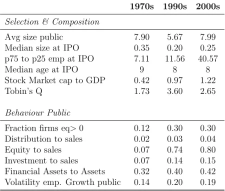
2.2 Empirical Evidence . . . 51

2.3 Model . . . 55

2.3.2 Public Firms . . . 60

2.3.3 Entry and Exit . . . 60

2.3.4 Timing . . . 61 2.3.5 Government . . . 61 2.3.6 Household . . . 61 2.3.7 Equilibrium . . . 63 2.3.8 Discussion . . . 64 2.4 Estimation . . . 66 2.4.1 Assigned Parameters . . . 68

2.4.2 Parameters estimated without solving the model . . . 68

2.4.3 Parameters estimated by solving the model . . . 69

2.4.4 Validation of the Model . . . 70

2.5 Quantitative Analysis . . . 73

2.5.1 Changes in Taxes and the Stock Market Boom in the 1990s . . . 73

2.5.2 What happened after 2000? Exploring other Channels . . . 84

2.6 Conclusion . . . 90

2.7 Appendix . . . 93

Appendix A. Data . . . 93

A.1. Data Sources . . . 93

A.2. Additional Empirical Facts about Public Firms . . . 95

Appendix B. Changes in Economic Environment . . . 100

B.1. Taxes . . . 100

B.2 Equity issuance costs . . . 105

B.3. Productivity shock process and production function curvature . . . 107

Appendix C. More on the model and its assumptions. . . 109

C.1. Privately Held versus Publicly Traded Firms . . . 109

C.2. The effect of taxes on optimal decisions . . . 115

C.3 Age profiles in the Model and the Data . . . 118

Appendix D. Further Results . . . 121

D.1. Decomposition of Results . . . 121

D.2 Changes in Equity Issuance Costs . . . 123

D.3. Sensitivity analysis . . . 124

1.1 Calibration Baseline Economy . . . 19

1.2 Calibration Results . . . 21

1.3 Non-targeted Moments . . . 22

1.4 Effects of Tax Reforms . . . 24

1.5 Summary Statistics Compustat . . . 33

1.6 Summary Statistics SDC Platinum . . . 35

1.7 Effects of Tax Reforms for different Entry Elasticities . . . 39

1.8 Tax Experiment with Elastic Labor Supply, τc= 0, financed by τd =τg =τr 40 1.9 Calibration Baseline Economy with AR(1) growth . . . 41

1.10 Calibration Results . . . 42

1.11 Economy with AR(1) shocks: Tax Reform setting τc = 0, financed by τd = τg =τr . . . 43

2.1 Main statistics . . . 52

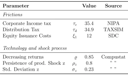
2.2 Assigned Parameters . . . 68

2.3 Parameters estimated without solving the model. . . 69

2.4 Targeted moments . . . 70

2.5 Non-Targeted moments . . . 71

2.6 Exogenous Changes . . . 74

2.7 From 70s to 90s: Changes in Taxes . . . 79

2.8 From 70s to 90s: Aggregates . . . 81

2.9 Publicly traded: Entrants vs Incumbents, Data vs Model . . . 82

2.10 Selection effect . . . 83

2.11 Exogenous Changes . . . 86

2.12 From the 70s to the 00s . . . 87

2.13 More statistics. . . 96

2.14 Publicly traded firms: entrants vs incumbents. . . 96

2.16 Employment Weighted Statistics . . . 97

2.17 Increase in Averages by Industry. . . 98

2.18 Estimated Tax Rates . . . 100

2.19 Summary table . . . 106

2.20 Estimation of the shock process . . . 109

2.21 Use of external equity by organizational form. . . 110

2.22 Decomposition and Changes in Equity Issuance Costs . . . 122

2.23 Sensitivity Analysis . . . 125

2.24 Calibration with full set of taxes . . . 130

2.25 Exogenous Changes in Taxes and equity Issuance Costs . . . 130

1.1 The Life Cycle of a Firm . . . 13

1.2 Employment growth by age in the model and the data. . . 22

1.3 Life Cycle of Firms . . . 29

1.4 Policy functions for different Z . . . 36

2.1 Trends in Publicly Traded Firms . . . 54

2.2 Timing of the Problem . . . 61

2.3 IPO choice for ρz = 0.8, σz = 0.23, κ= 5.5,η0 = 17.1 . . . 64

2.4 Dynamics around IPO . . . 73

2.5 IPO choice for givenθ, baseline (black) and after policy change (black and grey) 75 2.6 Life cycle and IPO choice of three firms in 70-80 and 90-00 . . . 76

2.7 Exit and Entry Rates into Publicly Traded . . . 99

2.8 Distribution taxes 1970-2008. . . 101

2.9 Corporate taxes 1970-2008. . . 104

2.10 Number of IPOs, Fraction of VC backed and Technological IPOs. . . 112

2.11 Dynamics around IPO of VC-backed and Non-VC-Backed . . . 113

2.12 Policies by years since IPO . . . 120

2.13 IPO choice, baseline low ρ . . . 126

Taxation and the Life Cycle of Firms

1.1

Introduction

The macroeconomic effects of the taxation of capital income have received a great deal of attention by economists and policy makers. Throughout modern economies the taxation of capital income takes many different forms: capital gains taxation, interest income taxation, dividend taxation, and corporate income taxation. In particular, the tax rate on corporate income in the US was until recently among the highest of OECD countries, and this has raised concerns about its effects on job creation and investment. Policy advisors from the Obama and Trump administrations have advocated for changes in the taxation of capital income and, indeed, the Trump administration has recently cut by nearly half the corporate income tax rate. In this paper, we study how different forms of taxing capital income affect investment and financing decisions of firms over their life cycle, as well as the creation of new firms (firm entry), aggregate capital accumulation and output. We then evaluate the effects of a tax reform that eliminates the tax on corporate income and replaces the lost revenue with a common tax rate on all other form of capital income.

Corporate profits distributed as dividends suffer from the so-called ‘double taxation’, since they are taxed both at the corporate and the personal income level (by the corporate income tax and the dividend tax, respectively). The literature has long emphasized that corporate income taxation diminishes investment by firms by reducing the after tax return on capital. In this paper, we show that these distortions are much more severe when firms’ growth over the life cycle is constrained by financial frictions. The impact of dividend taxation on firm investment decisions critically depends on the stage that firms are at in their life cycle, as young firms are more likely to issue equity while old firms are more likely to issue dividends. Young firms behave according to the ‘traditional view’ in the finance

literature: an increase in dividend taxation raises the cost of external equity financing, negatively affecting firms’ investment1_{. However, as emphasized by the ‘new view’ in the}

finance literature, dividend taxation does not affect investment decisions of firms distributing dividends (mature firms), since the dividend tax leads to an equiproportional reduction in the return and costs of investment. More generally, our paper stresses that the various ways capital income can be taxed (whether corporate income, dividend, or capital gains taxation) have quite different effects on investment and payout policies over the life cycle of firms, and hence on the life cycle growth of firms. They also have different and asymmetric effects on the market valuation of new versus incumbent firms, and thereby on firm entry.

Our paper is motivated by micro evidence on firm dynamics and the life cycle of firms. Haltiwanger et al. (2013) argue that start ups play a critical role for understanding US employment growth dynamics. The mass of firms entering the economy is large, most new businesses start as small but (conditional on survival) grow fast, and new entrants are important for understanding employment growth. Moreover, Hsieh and Klenow (2009) argue that the cross country differences in the life cycle growth of firms are important for understanding aggregate productivity differences across countries. The evidence indicates that firms face substantial equity issuance costs (seeHennessy and Whited(2007),Lee et al. (1996)). Using micro evidence from US and UK firms,Cloyne et al.(2018) show that financial frictions affect more strongly investment decisions of young firms than that of mature firms. Campbell et al. (2013) empirically document heterogeneous investment responses across young and mature firms after the reduction on shareholder taxes in the US in 2003. Becker et al. (2013) study many tax reforms on 25 countries over a 20 year period, finding that changes in payout taxes affect firms differently depending on their financial regime. Overall, this evidence points to the importance of modeling the life cycle of firms for assessing the effects of taxation. A model with a representative firm, as in the standard Neoclassical Growth Model, implicitly focuses on mature firms (i.e. those distributing dividends where the ‘new view’ holds), disregarding the evidence that investment responses to tax changes vary over the life cycle of firms. Moreover, the empirical findings ofHaltiwanger et al.(2013) suggest that it is important to consider the impact of taxation on business entry.

We extend theHopenhayn and Rogerson(1993) framework of firm dynamics to under-stand how different forms of taxing corporate income affect the life cycle of firms. We start by analysing a simple version of the model with a deterministic fixed level of productivity determined upon entry. Companies need to raise equity to set the firm up, starting their life in the ‘traditional view’ regime (equity issuance phase). They grow by accumulating profits (growing phase), until they reach their optimal size and start distributing dividends

rity phase). Consistent with the ‘new view’, dividend taxation does not distort investment decisions and dividends paid by mature firms. However, dividend taxation diminishes the optimal amount of initial equity issued by firms. Intuitively, firms can diminish the taxes paid by financing a larger portion of investments with retained earnings. Hence, dividend taxation reduces the initial size of firms, retarding the age at which they reach maturity, and diminishes entry. The taxation of capital gains has the opposite effects of dividend taxation. First, the taxation of capital gains encourages firms to issue more equity at entry in order to avoid paying the taxes that would accrue with the accumulation of internal funds. Second, it distorts the optimal scale of the firm at maturity. Corporate income taxation impacts on capital accumulation through several channels. First, corporate income taxation distorts the optimal size and dividends paid by mature firms by decreasing the return on capital. Second, crucial to our analysis and results, the corporate income tax decreases after-tax earnings, making it harder for firms to finance investment with retained earnings and causing firms to grow at a slower pace over their life cycle. As a result, the market value of the firm decreases, leading to two additional effects of corporate income taxation on capital accumulation: firms raise less equity at entry, and the equilibrium mass of entry becomes smaller. While these effects are also present under dividend taxation, they are stronger under corporate income taxation.

The baseline economy with firm dynamics (due to idiosyncratic productivity shocks at the firm level) is calibrated to moments on the micro data on firms’ investment and financing decisions. We use the calibrated model economy to quantitatively assess the effects of a reform that eliminates the taxation of corporate income while keeping constant the tax revenue collected on capital. This is done by finding the common tax rate (τ) on all forms of capital income (dividends τd, interest income τr, and capital gains τg) that collects the

same tax revenue as in the baseline economy. The purpose of the proposed policy reform is twofold. Firstly, all sources of capital income are treated symmetrically from the household perspective. Secondly, by eliminating the corporate income tax, financially constrained firms are able to accumulate profits and to reach maturity (the dividend distribution stage) faster. The elimination of the corporate income tax in the baseline economy (τc = 0.34) should be

accompanied by an increase in the other capital income tax rates to 0.41 in order to keep government revenue constant (the dividend and capital gains tax in the baseline economy were set to 0.15 and the interest income tax was set to 0.25). In equilibrium, this leads to an increase in the initial size at entry, a decrease in the optimal size at maturity, and a decrease in the time to reach maturity. This benefits mostly young firms, thereby increasing entry by 35%. Aggregate output increases 12%, accompanied by a large increase in the aggregate capital stock (32%). Hence, the large response of firm entry is important for understanding

the macroeconomic effects of the tax reform. When entry is kept fixed, the increase in output is a third and the rise in capital is half of those in the economy with endogenous entry.

At the heart of our results is the fact that the tax reform increases the expected value at entry more than the value of incumbent firms, leading to a reallocation of resources from mature to younger firms, which operates through an increase in entry and in the equilibrium wage rate. The elimination of corporate income taxation allows financially constrained firms to retain a larger fraction of their earnings and increase their investments. The ability to re-tain earnings is particularly relevant for young firms, which are more likely to be constrained than the average incumbent firm in the economy. Since the value at entry is determined by the average value of age-0 firms, the value of the average firm entering the economy increases more than that of incumbent firms when corporate income taxation is eliminated. In general equilibrium, the increase in the value of entry requires the wage rate to rise, which reduces labor demand by incumbent firms. Labor market clearing requires a larger mass of firm entry, which rises by about 35%. Larger firm entry, together with a reallocation of resources to financially constrained firms, lead to an increase in aggregate TFP of 4.6%.

Our model economy builds onGourio and Miao (2010), who study the impact of divi-dend taxation on firms’ investment and payout decisions. We contribute by comparing alter-native forms of capital income taxation and by extending their analysis to incorporate three key features for our results: life cycle (endogenous entry), financial frictions, and corporate income taxes. In particular, we emphasize the importance of the life cycle of firms for un-derstanding how taxation affects investment incentives of firms. Korinek and Stiglitz(2009) build a theory of the life cycle of firms for understanding the impact of dividend taxation but abstract from corporate income taxation and firm entry. McGrattan and Prescott (2005) and Atesagaoglu (2012) study how corporate income taxation affects the market valuation of firms in environments with a representative firm. Conesa and Dom´ınguez (2013) advo-cate for the elimination of corporate income taxation in a Ramsey optimal taxation exercise with a representative firm, with no financial frictions and no firm entry/exit. Similar to us, Anagnostopoulos et al.(2015) evaluate the gains of eliminating corporate income taxation in a model with firm heterogeneity and household heterogeneity. We abstract from household heterogeneity but contribute by focusing on firm entry and the life cycle of firms, which turn out to be key for the large quantitative effects of our tax reform, and which Haltiwanger et al. (2013) emphasize as crucial for understanding the dynamics of employment growth in the US. The financial crises has sparked great interest in the literature analyzing the role of financial frictions in business cycle fluctuations. Papers in this literature include Coo-ley and Quadrini (2001), Khan and Thomas (2013), Jermann and Quadrini(2012) (among many others). Our results suggest that the design of capital income taxation may affect the

propagation of business cycle shocks.

An outline of the paper follows. Section2.3presents and analyzes a simple version of our baseline model economy in which firms do not face idiosyncratic shocks to their productivity, in order to illustrate how different forms of taxing capital income affect investment and payout policies over the life cycle of firms, the value of firms to its shareholders, and firm entry. Section 1.3 presents our baseline model economy of firm dynamics and taxation of capital income, and shows the calibration and our main quantitative exercises. Section 1.4 concludes2.

1.2

A Simple Deterministic Model Economy

Our baseline model extends theHopenhayn and Rogerson(1993) framework of firm dynamics to study taxation of corporate capital income. Time is continuous3_{. Each firm may exit the}

economy with some fixed probability. The entry of new firms is endogenous. Firms can finance investment with retained profits or equity issuance. Firms face adjustment costs in capital. Following Cooley and Quadrini (2001) and Gomes (2001), firms face financial frictions, since equity issuance is costly. There is a representative household that owns all firms. There is a large number of firms so that the representative consumer does not face any uncertainty. As in Gourio and Miao (2010), households pay taxes on dividends (τd),

interest income (τr), and capital gains taxes (τg)4. In addition, corporations pay taxes on

corporate profits (τc), so that capital income is taxed both at the firm and household level.

In this section, we illustrate the key ideas of our paper in a deterministic version of our baseline model economy that abstracts from adjustment costs in capital.

1.2.1

The problem of a firm

When firms are created, they draw a productivity z that stays fixed over the lifetime of a firm. Firms exit exogenously the economy at a rate δd. The economy is a steady state with

an after tax interest rate equal tor(1−τr) =ρ, where ρis the rate of time preference of the

representative household (investor).

2_{AppendixD evaluates the sensitivity of the results to alternative formulations of entry decisions, the}

shock process faced by firms, and to incorporating an endogenous labor supply choice.

3_{Achdou et al.(2017) and Barczyk and Kredler(2014) advocate the use of continuous time models for}

analyzing heterogeneous agent models. We extend their methods to a model of firm dynamics with financial frictions.

4_{While in the US capital gains are taxed upon realization, we follow standard practice in the literature by}

modeling capital gains taxation on an accrual basis. This modeling choice simplifies the analysis considerable and allow us to derive our results in a more transparent way.

Each firm produces output with a decreasing returns to scale production function in capital and labor inputs: f(z, k, n) =z1−α−η_kα_nη_{. Profits are given by}

π(z, k) = max

n {f(z, k, n)−wn−δk}.

The flow constraint is

˙

k= (1−τc)π(z, k)−d+ (1−ξ)e,

wheredandedenote dividend distribution and equity issued by firms. We assume that equity issuance is costly. There is a cost ξ per unit of equity issued, so the resources available are

e(1−ξ).

Consider a firm with fixed z. The market value (V), the dividends paid (d), and the equity issued (e) are deterministic functions of the age of the firmt. However, these variables are not explicitly indexed with a subscript t to simplify the notation (unless there is some risk of confusing the reader). Taking as given investment and financial policies, the market value of the firm V is such that the after tax rate of return on equity equals the investor rate of discount ρ:

ρ= d(1−τd) + (1−τg)( ˙V −e−δdV)

V (1.1)

where ˙V represents the rate of change of V with respect to time (age of the firm). Note that increases in share values due to equity issuance are not taxable. Firm exit gives rise to negative capital losses that are tax deductible. The above non-arbitrage equation can be re-arranged as ρ 1−τg +δd V = 1−τd 1−τg d−e+ ˙V .

The solution to this first-order linear differential equation on V gives the integral in (1.2). Note that the path of dividends in this integral is multiplied by the ratio 1−τd

1−τg, which follows

from the interplay of two opposite effects of the taxation of dividends and capital gains. The numerator is explained by the fact that investors receive a fraction 1−τd of the dividends

distributed by the firm. The denominator is explained by the fact that when firms retain earnings (do not distribute dividends) the value of the firm increases and this capital gain is subject to the tax τg. In addition, the rate at which firms discount future dividends

(₁₋ρ_τ

value of the firm over time and these changes in market value are taxed at a rateτg.

The problem of the firm in state (z, k) is then to choose investment and financial policy to maximize: V(z, k)≡max Z ∞ 0 e−( ρ 1−τg+δd)t 1−τd 1−τg d−e dt (1.2) subject to: ˙ k = (1−τc)π(z, k)−d+ (1−ξ)e d≥0, e≥0, k0 given.

Associate the present-value multipliers e−(

ρ 1−τg+δd)_λ

t to the flow of funds constraint,

e−(

ρ

1−τg+δd)_µe

t to the non-negativity constraint on equity issuance, and e

−(₁₋ρ_τg+δd)

µd_t to the non-negativity on dividend distribution. Then, the FOC from the Maximum Principle imply:

λ= 1−τd 1−τg +µd (1.3) (1−ξ)λ+µe = 1 (1.4) λ ρ 1−τg +δd−(1−τc)π0(z, k) = ˙λ (1.5) ˙ k = (1−τc)π(z, k)−d+e(1−ξ) (1.6) µd≥0, d≥0, µd_td= 0 (1.7) µe≥0, e≥0, µe_te= 0 (1.8) lim t→∞e −(₁₋ρ_τg+δd)t λtkt = 0 (Transversality) (1.9)

Conditions (1.3) and (1.7) imply that the shadow value of fundsλ≥ 1−τd

1−τg, with equality

if dividends are strictly positive. Conditions (1.4) and (1.8) imply that the shadow value of fundsλ≤ 1

1−ξ, with equality if equity issuance is strictly positive. In sum, the shadow value

of funds satisfies λ∈h1−τd 1−τg, 1 1−ξ i .

1.2.2

Entry, optimal initial equity, and time to maturity

As in Hopenhayn and Rogerson (1993), firms pay a fixed cost ce to draw a productivity z

from an exogenous probability density ge. The firm decides the initial amount of capital

k0(z) after observing the productivity draw z. The value of entry is then given by

Ve = Z ∞ 0 V(z, k0(z))− 1 1−ξk0(z)ge(z)dz =ce, (1.10)

where the second equality states that in a steady state equilibrium the value of entry should be equal to the entry cost. The wage rate adjusts to ensure that this is the case. The mass of firms entering the economy is determined by the labor market clearing condition:

Z ∞

0

n(z, k)g(z, k)dzdk = 1,where g satisfies (1.11) 0 = −∂k(s(z, k)g(z, k))−δdg(z, k) +M ge(z)Ik=k0(z),

where n(z, k) denotes the optimal labor demand, ˙k = s(z, k) is the optimal investment in capital, and g(z, k) the mass of firms in state (z, k).

Consider a firm with productivityz that raises capital (equity) k0 when newly created.

The firm will accumulate capital until it reaches the optimal amount of capital k∗(z). Once the firm reaches its optimal scale, it distributes dividends until it dies. The age (T) at which the firm starts distributing dividends solves the following equation:

(1−τc)

Z T

0

π(z, kt)dt+k0 =k∗. (1.12)

The above equation defines an implicit function T(z, k0) characterizing the age when a firm

matures (starts distributing dividends) as a function of its net worth at entry (age 0). Since an increase in initial capital k0 increases the profits accumulated by the firm over time, the

firm takes a shorter period to reach maturity. Formally, differentiating (1.12) with respect to initial capital k0 yields

dT dk0 =−1 + (1−τc) RT 0 π 0_{(z, k} t)_dk0dktdt (1−τc)π(z, kT) <0. (1.13)

In words, if initial capitalk0 is greater, everything else held constant, the time to reach

maturity decreases.

We now focus on determining the optimal amount of initial equity. For a fixed value of

k0, T is computed from (1.12). Equations (1.3)- (1.7) imply that the shadow value of funds

at age T satisfies λ(T) = 1−τd

1−τg. Integrating (1.5) between 0 and T(k) gives

λ(0) = 1−τd 1−τg e RT 0 h (1−τc)π0(z,kt)−(₁₋ρ_τg+δd) i dt . (1.14)

The function inside the integral in (1.14) has a positive sign for allt < T, is equal to 0 at T, and is decreasing in k0 (due to decreasing returns to capital accumulation). Moreover,

function of k0. The optimal value of initial equity is obtained by solving λ(0) = 1 +ξ.

The value of a firm with initial capital (equity) k0 satisfies

V(z, k0) = Z ∞ T(k0,z) 1−τd 1−τg e−( ρ 1−τg+δd)t d∗(z)dt = 1−τd 1−τg d∗(z)e −(₁₋ρ_τg+δd)T(z,k0) ρ 1−τg +δd . (1.15) Note that another way of solving for the optimal amount of initial equity is

max k0 V(z, k0)− 1 1−ξk0, (1.16) which implies V0(z, k0) = 1−τd 1−τg d∗(z)e−( ρ 1−τg+δd)T(z,k0)₍₋₁₎dT dk0 = 1 1−ξ. (1.17)

Since V is a concave function of capital, it follows that the solution for initial equity is unique.

1.2.3

The life cycle of a firm

The previous discussion highlights that, as inKorinek and Stiglitz(2009), firms in our simple model face three distinct phases during their life cycle: equity issuance phase, growth phase, and dividend distribution phase.

• Equity issuance phase. The first stage occurs when firms are created. Firms start with zero net worth. In order to operate they need to raise equity at age 0 so that

e0 > 0. The Kuhn Tucker complementarity slackness condition (1.8) implies that

µe

0 = 0 so that (1.4) implies that the shadow value of assets at age 0 is given by

λ0 = ₁₋1_ξ. The non-negativity constraint on dividend distribution binds (µd0 > 0) so

that firms do not distribute dividends. The amount of initial equity raised is such that: (1−τc)π0(z, k0)>

ρ

1−τg

+δd (1.18)

By equation (1.5), once the firm is set up and λ0 = ₁₋1_ξ, the next instant the value

of the multiplier is decreasing, i.e. limt→0+λ_t < 1

1−ξ . Otherwise, condition (1.18)

implies that limt→0+λ_t > 1

1−ξ, which violates the non-negativity of µ e

t (see equation

(1.4)). This phase would fall within the so-called ‘traditional view’, where firms are using equity issuance as the marginal source of financing.

• Growth phase. When firms start operation (immediately after age 0), the continuity of λt together with (1.18) imply that the shadow value of net worth decreases since

(1−τc)π0(z, kt)> ₁₋ρ_τg +δd for t > 0 in the right neighborhood of t = 0 ( ˙λt). Newly

created firms start operating and retain earnings in order to increase their capital. As capital grows, the shadow value of funds decreases, relaxing the non-negativity constraint on dividends (its multiplier decreases).

• Dividend distribution phase. Firms reach the dividend distribution phase (matu-rity) when the shadow value of funds reaches the value 1−τd

1−τg. At this stage, the marginal

source of funds is retained earnings, and its marginal cost equals the marginal benefit of distributing dividends. Growth ceases when firms reach a steady state with a constant capital (k∗) and constant dividend distribution d∗ satisfying

(1−τc)π0(z, k∗) =

ρ

1−τg

+δd (1.19)

(1−τc)π(z, k∗) = d∗ (1.20)

1.2.4

Discussion on taxation and the life cycle of firms.

We now discuss, for a fixed wage rate, the effects of taxes on the life cycle of firms. Equations (1.19) and (1.20) determine the optimal level of capital (k∗) and dividends (d∗) by mature firms. The value of a mature firm with productivity z is

Vmature(z) = 1−τd

ρ+δd(1−τg)

d∗. (1.21)

Using (1.15), the value of an age-0 firm with productivity z satisfies

Vnew(z) = 1−τd ρ+δd(1−τg) d∗ | {z } Vmature_(z) e−( ρ 1−τg+δd)T(z,k0) _(1.22)

The value of a new firm is a fraction of the value of a mature firm and that fraction decreases with the time it takes to reach maturity. Below we use (1.19)-(1.22) to evaluate the impact of capital income taxation on mature firms and on the market value of mature firms relative to that of age-0 firms.

Dividend taxation (τd) The tax rate on dividend distribution does not affect equations

dividends paid by mature firms, a result consistent with the “new view” of the public finance literature. When the firm is indifferent between using its marginal unit of funds as dividend or investment, a change in the dividend tax rate has proportional effects on the benefits and cost of investment. As a result, investment decisions and dividend payouts of mature firms are unaffected by the dividend tax rate. However, the dividend tax reduces the market value of mature firms (it changes proportionally with the term 1−τd, as shown in (1.21)).

Paradoxically, the dividend tax rate affects capital accumulation when firms are not paying dividends. This is because the lower value of the firm to shareholders reduces the optimal amount of initial equity (see equation (1.17)), retarding the age at which firms reach maturity. Intuitively, the firm can effectively diminish the taxes paid by reducing (initial) equity issuance and by financing investment with retained earnings. The fact that the firm reaches maturity at a later age, implies that dividend tax rate decreases the market value of firms at entry more than at maturity (in (1.22) the increase in T caused by dividend taxation further reduces the value of entry).

In sum, while dividend taxation does not distort the optimal scale and payouts of ma-ture firms, it distorts the initial scale of operation of firms, diminishing capital accumulation along the life cycle and the age at which firms reach maturity. Moreover, dividend taxation affects assymmetrically the market value of mature firms versus that of entrants which, in general equilibrium, will negatively affect the creation of businesses (entry).

Taxation of capital gains (τg) The taxation of capital gains (τg) increases the cost

of equity financing (₁₋ρ_τ

g), reducing capital and dividend distribution of mature firms (see

equations (1.19) and (1.20)). The decrease in dividends implies a decrease in the market value of mature and young firms5_{. The capital gains tax has two opposite effects on the initial}

capital of firms. On the one hand, when capital gains tax increases, the return on holding firms’ shares needs to increase to satisfy the non-arbitrage condition. Since technology features decreasing returns, this is attained by reducing the optimal size of the firm. This, in turn, reduces the optimal initial size. On the other hand, the capital gains tax stimulates equity issuance at entry by increasing the rate at which future dividends are discounted (note that ₁₋ρ_τ

g +δd increases with τg). Intuitively, by raising more equity at entry, firms avoid

paying taxes on capital gains that would accrue with the accumulation of internal funds.

5_{Note thatτg enters in the denominator of (1.21). This expression represents the fact that the market}

value of mature firms increase withτg because the tax code in our model economy allows for a tax credit associated to the death of the firm. Quantitatively, this effect will likely have a small effect on the market value of firms if the death rate is small. As a result, we should expect the market value of mature firms to move together with d∗. This is always the case if we assume that there is no tax credit associated to the capital losses upon death of firms.

Note that this result is the opposite of what we found for dividend taxation.6

Corporate income taxation (τc) Corporate income taxation reduces capital

accumula-tion and dividends paid by firms. Intuitively, corporate income taxaaccumula-tion reduces the after tax benefit to capital (see left hand side of equation (1.19)) but without reducing the cost of funds to the firm. This effect reduces the optimal size (k∗ decreases) and distributions (d∗) by mature firms (see equation (1.20)). Lower dividends imply a decrease in the market value of mature firms (see equation (1.15)) which, in turn, decreases the optimal amount of initial equity (equation (1.17)). Hence, firms start their life with a smaller scale. Moreover, the firm grows at a slower pace since the corporate income tax reduces the fraction of earnings that the firm accumulates during its growth phase in the life cycle (see equation (1.12)). The time to reach maturity may increase or not with corporate income taxation since there are two opposite forces at work: while firms grow more slowly, their optimal scale is smaller. In our computational experiments, the first effect is stronger so that firms take a longer time to mature.

It is important to note that the decrease ind∗associated with corporate income taxation reduces proportionally the market value of firms at entry and at maturity. In addition, for a fixed amount of initial equity, the corporate income tax makes it harder for firms to accumulate retained earnings, retarding the age at which firms reach maturity. This additional effect implies that corporate income taxation affects more negatively the market value of firms at entry than at maturity. The asymmetric effect on market valuations at entry and at maturity implies that the corporate income tax discourages entry, an effect that will play an important role in the tax reform, and that is analyzed in the next section of the paper.

Quantitative illustration We parameterize the simple model in order to illustrate the discussion on how various forms of taxing capital income affect the life cycle of firms7_{. We}

simulate in partial equilibrium (e.g. fixed wage rate) the life cycle of a firm in three different scenarios: under the baseline parametrization, and after an increase of 5 percentage points in each of the tax rates, maintaining everything else constant. Figure 1.1 plots the life cycle profile of capital for the four cases considered. Consistent with our discussion above,

6 _{Recall that, in order to minimize taxes on dividends, dividend taxation encourages young firms to}

finance investment with internal funds.

7_{We set the following parameters for the production function α = 0.3 ×0.85, η = 0.7×0.85. The}

depreciation of capital is fixed as δ = 0.05 and the rate of time preference is set so that the steady state interest rate is 4% (r= 0.04). The equity issuance cost is set to 0.10. The wage rate is fixed at 1. Taxes in baseline areτc= 0.34,τd= 0.15,τg= 0.15 andτr= 0.25

firms start their life cycle with a lower amount of capital when they are subject to dividend or corporate income taxation. The initial level of capital is slightly lower under dividend taxation than under corporate income taxation. While the level of capital at maturity is not affected by dividend taxation, it is negatively affected by corporate income taxation. This is the key factor explaining why it takes the firm about one more year to reach maturity under dividend taxation, despite the fact that the firm is able to accumulate capital faster under dividend taxation than under corporate income taxation. The latter explains why the age profile of capital in the figure is steeper under dividend taxation than corporate taxation.

It is interesting to compare the effects of dividend taxation with those of capital gains taxation. While dividend taxation does not distort capital accumulation of mature firms, it has a large negative impact on the initial amount of equity at entry. In this way, the firm finances a larger portion of its investment over the life cycle with internal funds, diminish-ing the present value of taxes paid on dividends. Capital gains taxation does precisely the opposite. It encourages firms to finance a bigger fraction of their investment with external equity, diminishing firm growth over the life cycle, and the present value of taxes paid on capital gains. In terms of capital accumulation, the trade-off is between distorting invest-ments prior to becoming mature (dividend taxation) versus distorting the optimal scale at maturity (capital gains taxation). The corporate income tax distorts investment decisions all through the life cycle.

Figure 1.1: The Life Cycle of a Firm

1 1.5 2 2.5 3 Capital 0 2 4 6 8 Years Baseline Δτc=5pp Δτd=5pp Δτg=5pp

Life cycle of three identical firms in equilibriums with different taxes. Blue is the baseline: τc= 0.34,τd= 0.15,τg= 0.15 andτr= 0.25. Changes after an increase of 5pp of each of the tax rates, maintaining everything else constant.

1.3

The Stochastic Model Economy

The simple model is extended as follows. Following the standard theory of investment, we introduce adjustment costs in capital and uncertainty in productivity. Physical capital evolves according to

˙

k =x−δk.

and the resource cost of investingx is given by x+ Ψx_2k2, where the second term reflects the presence of adjustment costs in capital.

The productivity of a firm (z) follows a geometric Brownian Motion

dz =µzdt+σzdW, (1.23)

where µ determines the drift and dW is a Wiener process. Since productivity follows a geometric Brownian motion, large firms in our model follow Gibrat’s Law and growth rates are independent of firm size. Empirical research, such asHall(1987), suggests that Gibrat’s Law is a good approximation for firms that are not too small (see also Gabaix (2009)). Similar specification of the productivity shocks has been widely used in the literature on firm dynamics (see Atkeson and Kehoe (2005), Luttmer (2007), Da-Rocha et al. (2017), among many others)8_.

The flow of a firm at timet in state (z, k) with investing expenditures x is given by

d−e(1−ξ) = (1−τc)π(z, k)−x−Ψk x2 2k, (1.24) where π(z, k) = max n {y(z, k, n)−wn}.

8_{Nonetheless, in AppendixD.3of the paper we consider the robustness of our results to an alternative}

The firm in state (z, k) solves the following optimal control problem: v(z, k) = maxE0 Z ∞ 0 1−τd 1−τg d−e e−( ρ 1−τg+δd)t_{dt (1.25)} subject to: dz =µzdt+σzdW (1.26) ˙ k =x−δk (1.27) d−e(1−ξ) = (1−τc)π(z, k)−x−Ψk x2 2k +τcδk, (1.28) where ₁₋ρ_τ

g +δd is the rate at which the firm discount future payments to/from shareholders

when acting in their interest (see Appendix A).

The Hamiltonian-Jacobi-Bellman equation of a firm satisfies:

ρ 1−τg +δd v(z, k) = max1−τd 1−τg d−e+∂kv(z, k) ˙k+µzz∂zv(z, k) + (zσ)2 2 ∂zzv(z, k). (1.29) Upon entry, firms draw the initial productivityz0 from a Pareto distribution:

ge(z0) =    1 z₀+1 if z0 >1 0 otherwise. (1.30)

The initial amount of equity raised by a firm that draws z solves the following problem: ˆ

k0(z0) =k0 {v(z0, k0)−

1

(1−ξ)k0} (1.31)

Then, the value of entry for a firm that draws z can be expressed as

ve(z0) =v(z0,kˆ0(z0))−

1 (1−ξ)

ˆ

k0 (1.32)

In equilibrium the free entry condition requires

Ve ≡ Z ∞ 1 ve(z0)ge(z0)dz0 = Z ∞ 1 ve(z0) 1 z₀+1 ≤ce, (1.33)

with strict equality if there is positive entry.

g of firms in state (z, k) satisfies: 0 = −∂k(s(z, k)g(z, k)) − ∂z(µzzg(z, k)) + σ2 z 2 ∂zzg(z, k) −δdg(z, k) + M ge(z)Ik=k0(z), (1.34) where s(z, k) = ˙k =x−δk and M denotes the mass of firms entering the economy.

In the presence of uncertainty, shocks to firms’ productivity may change their financial regimes over the life cycle. A firm that is increasing its capital and issuing equity, may stop doing so if productivity decreases. When productivity decreases by a large amount, the firm may even start distributing dividends and disinvesting. Conversely, an increase in productivity may move the firm back to the equity issuance and investment regime. AppendixC provides a detailed discussion on firms’ investment and financial policies in the presence of uncertainty and adjustment costs.

There is a representative household that owns the market portfolio of firms. Households supply labor to firms, receive dividends, buy/sell shares of firms, and trade bonds. Since households do not face uncertainty on their savings, in equilibrium there is a no arbitrage condition (see Appendix A for its derivation) that equates the after-tax return in bonds to the expected after-tax return in each firm. Households pay personal income taxes on earnings (τw) and interest income on bonds (τr). The government rebates the aggregate tax

revenue to the representative household with a lump sum transfer (T).

The representative household maximizes the discounted lifetime utility subject to the intertemporal budget constraint

max {ct} Z ∞ 0 e−ρtu(ct)dt (1.35) subject to: (1.36) Z ∞ 0 e−r(1−τr)t_(c−(1−τ w)w−T) =a0, (1.37) a0 = Z v(z, k)g(z, k)dzdk, (1.38) wherea0 is the period-0 market value of all firms. In steady state equilibrium,rt(1−τr) = ρ

and ct =c∀t. Note that given that firms cannot borrow, the assumption of a representative

consumer implies that bonds are in zero net supplyb0 = 0 and households make zero interest

income9.

9_{AppendixD.2 evaluates the sensitivity of the results when an endogenous labor labor supply choice is}

Definition of steady state equilibrium Given a fiscal policy (τw, τr, τc, τg, T), a

steady state equilibrium is given by value functions for incumbent firms (v(z, k)), value of entryVe_{, prices (w, r), firms policy functions on employment (n), investment in physical (x)}

and financial policies (d, e) , initial equity k0, mass of entry M, measure of firms g(z, k),

consumption cand initial household assets a0 such that:

1. Given prices, the value functionv(z, k) satisfies the HJB equation of the firm and firm decisions (n, x, d, e) are optimal.

2. Ve _{satisfies the free entry condition (1.33).}

3. The government budget constraint is satisfied (all tax revenue is rebated back to con-sumers as a lump sum transfer).

4. Households maximize utility taking as given government transfer, prices, and initial wealth, which implies that steady state consumption is equal to permanent income:

c=ρa0+w+T.

5. Labor, bonds, and goods market clear

Z n(z, k)g(z, k)dzdk = 1 c+ceM + Z x+ψx 2 k g(z, k)dzdk = Z z1−α−γkαnγg(z, k)dzdk. (1.39)

1.3.1

Quantitative Analysis

The calibration targets aggregate and firm level data from the US economy. In principle, our goal is to target all US businesses that pay corporate income taxes. The calibration requires targeting “dynamic moments” from US firms, such as average firm growth, volatility and autocorrelation of investment rates over time. We follow Gourio and Miao (2010) in using Compustat data to pin down these calibration targets. Hence, the calibration strategy implicitly assumes that privately held businesses and publicly traded companies are alike with regards to employment growth, investment rates, and equity issuance by privately held businesses. The key difficulty is that there is very limited longitudinal data on private corporations. However, Haltiwanger (2006) provides evidence that both private and public firms face a life cycle in which net employment growth tends to be higher for young firms than mature firms even when controlling for firm size. Moreover, Asker et al.(2011) analyze

a new data set on private US firms and find that firm growth, investment, return on assets are similar across private firms in this database and public firms in Compustat. To the extent that private corporations face a higher cost of external financing, the former type of firms should gain more than the latter from reducing corporate income taxes.

We also target cross-sectional data on the size distribution of businesses from the US Census Bureau. Now, the universe of US businesses include private pass-through businesses that are not subject to the US corporate income tax (S corporations, partnerships).10 Since most of these businesses tend to be small, as a compromise we target data on the size distribution of businesses that includes businesses with more than 50 employees. The set of parameters to be calibrated is divided in two groups.

Parameters assigned without solving the model. The tax parameters are from the Internal Revenue Service (year 2015). The corporate income tax rate is 34% (τc= 0.34)11.

The capital gains tax rate is set to 0.15 (τg = 0.15), the dividend tax rate to 0.15 (τd= 0.15),

and the personal income tax rate to 0.25 (τr = 0.25, τw = 0.2512), which corresponds to

the marginal Federal taxes faced by a married couple with the average household income in the US. Households are assumed to discount future utility at an annual rate of 0.0375 (ρ = 0.0375) so that the (before tax) steady state return on capital is 5%, consistent with the estimates of the return on capital by Cooley and Prescott (1995). The parameters on the production function are set to standard values in the literature: the profit share is set to 0.15, with 70% of the remaining share going to labor and 30% to capital (α = 0.85∗0.3, η = 0.85∗0.7), as in Midrigan and Xu (2014). The depreciation rate of capital is set at 0.05 per year (δk = 0.05). Based on data from US Census Bureau’s Business Dynamic

Statistics (BDS), the average annual exit rate of firms with more than 50 employees is 4.6%, so δd = 0.046. Using data from Thomson Reuter’s Securities Data Company (SDC)

Platinum, we find that during the period 1995-2015 the total costs of equity issuance as a percentage of proceeds is about 7%13_{. This is computed following closely the procedure of} Lee et al. (1996) for IPO firms. It is somewhat smaller than the ones reported by Hennessy and Whited (2007), who estimated equity issuance cost in the range of 8.3% to 10.1%. Hence, the cost of raising external funds is set to 0.07 (ξ= 0.07). Nonetheless, firms raising their initial capital at entry face a higher equity issuance cost ξe. This parameter will be

determined later by simulating the model economy. Our calibration requires that ξe >0.07

10_{Developing a theory of organizational choice (pass through entities versus C corporations) is outside}

the scope of the current paper. SeeDyrda et al.(2018) for a theory of organizational choice.

11_{The progressive rate structure of the federal corporate tax in the US is designed such that it produces}

a flat 34% tax rate on incomes from $335,000 to $10,000,000, gradually increasing to a flat rate of 35% on incomes above.

12_{Labor income tax rate is kept constant in all experiments.} 13_{See AppendixB.2for more details on the data and computation.}

in order to match the equity issuance by incumbent firms.

Parameters assigned by solving the model. It remains to assign the parameters driving the stochastic process on productivity (µz, σz), the parameter Ψ driving adjustment

costs, the productivity distribution of firms that enter the economy and their cost of raising external capital. Entering firms draw their initial productivity from a Pareto distribution with tail parameter ηp and a location parameter 1 (the lowest possible productivity is one).

The wage rate is normalized to 1, and the fixed cost of entry is set equal to the value of entry.

Targeted moments. Although the endogenous equilibrium outcomes of interest will be jointly determined by all of these parameters, each of these parameters is intuitively connected with a particular moment of interest. The parameter µz is closely connected with

firm growth andσzwith the variance of investment. The parameter Ψ is closely related to the

correlation of investment rates across two consecutive years and the parameter determining the Pareto tail with the size distribution of businesses. Finally, the cost of raising initial equity is closely connected to the amount of external finance by incumbent firms. With these connections in mind, the following statistics are targeted:

1. An average annual employment growth of 2.1%.

2. The volatility of the investment rate (x/k) among firms of 0.059.

3. The autocorrelation of investment rates between two consecutive years of 0.57. 4. The ratio of equity issuance by incumbent firms to investment of 12.6%.

5. The size distribution of businesses, computed using data from BDS and reported in Table 1.2.

The first 4 targets are computed using Compustat data from over the period 1995-2015.14 _{For the reasons previously discussed, in computing the size distribution of businesses}

we abstracted from small businesses in the BDS and focused on businesses with more that 50 employees. Tables 1.1 and 1.2 show the parameter values and the calibration results.

Parameter values and discussion. The model accounts well for the targeted mo-ments. The baseline economy matches the average employment growth of 2.1 percent in the data. Recall that productivity in our model economy follows a geometric Brownian Motion with a drift given by µ = µz + σ

2 z 2

15_{. Hence, the variance of shocks is a force driving firm} 14_{See AppendixB.1for more information about the data and variable construction.}

15_{This follows from Ito’s lemma, and the specification of the process of productivity growth in our model,}

Table 1.1: Calibration Baseline Economy

Parameter Description Value

ψ Capital adjustment cost 0.09

µ Productivity drift -0.00325

σ Volatility of prod. shock 0.15

ξe Financing cost at entry 0.30

ηp Distribution of businesses 1

growth.16 The model economy accounts for the 2.1% in average employment growth with

µz = −0.00325. To measure the volatility of the investment rate and its autocorrelation

over time in our baseline economy, we first solve the model to compute the stationary dis-tribution of firms. Then, we draw firms from this disdis-tribution and simulate them over the year to compute annual investment rates. The annual volatility of the investment rate in the baseline economy is 0.054, which is close to the value of 0.059 in the data. Matching this target requires a significant variance in productivity since σz = 0.1517. The

parame-ter ψ = 0.07 is set to match the autocorrelation of annual investment rates over two years across the stationary distribution of firms. This parameter is between the 0.049 estimated byCooper and Haltiwanger (2006) and the 1.08 value obtained byGourio and Miao(2010). The size distribution of businesses in the baseline economy is determined by the distribution of businesses at entry and by the stochastic growth in productivity over the life cycle of firms. The model accounts reasonably well for the size distribution of businesses, although the match is not perfect. The model implies that 50 percent of businesses have fewer than 100 workers, and 22 percent of businesses employed between 100 workers and 250 workers. The corresponding fractions in the data are 53% and 29%. The fraction of businesses with more than 5,000 employees are about 0.6% in the model economy and 1% in the data18_.

A crucial parameter in our model economy is given by the cost of external financing. As inKorinek and Stiglitz(2009), financial frictions matter for the different financial regimes that firms go through their life cycle19_{. In particular, we want our model economy to be} 16_{Moreover, the distribution of productivity at entry is such that most businesses in our baseline economy}

start their life with a low productivity level, not far from the minimum value of 1, which represents a low barrier on z.

17_{Nonetheless, recall thatzin the production function is raised to the power of 0.15 so that the variance}

of TFP is much smaller than the one in z. For instance,Gourio and Miao(2010) estimate a variance in TFP of 0.2, though in their model TFP follows an autoregressive process with persistence of about 0.8

18_{In the data, most large firms are multi-establishment, a fact that our model cannot account for. This}

is the main reason our model underpredicts mass in largest size category.

19_{Gourio and Miao(2010)’s model abstracts from financial frictions and life cycle. Firms in their model}

go through different financial regimes because of the differential tax treatment on dividends and capital gains during the year 2003.

consistent with data on firm growth, investment rates, and the fraction of investment financed by raising capital on the equity market. Recall that the cost of external finance was set exogenously at 7 percent using data from SDC Platinum. The model economy matches the 13 percent target for the fraction of investment financed by equity issuance among incumbent firms. To match this statistic, the model requires that firms at entry face substantial financial frictions. The baseline economy assumes that when firms enter the economy they face equity issuance costs of 0.30. Lower values of equity issuance costs at entry imply that firms raise a substantial amount of equity when they enter in order to invest a large amount and avoid adjustment costs in capital as they grow (in expectations) over their life cycle. While we do not have data on the cost of raising external funds when firms are created, we find that the cost of raising external funds in initial public offerings in the SDC data is about 12%. Presumably, the cost of raising external funds when businesses are actually created should be much larger. Moreover, our model assumes that firms learn their productivity before making the initial investment in capital. Firms in our model would invest less when they enter if they face some uncertainty on their initial productivity and learn it over time. Hence, our calibrated equity issuance cost at entry may be capturing the effects of information frictions that our model abstracts from.

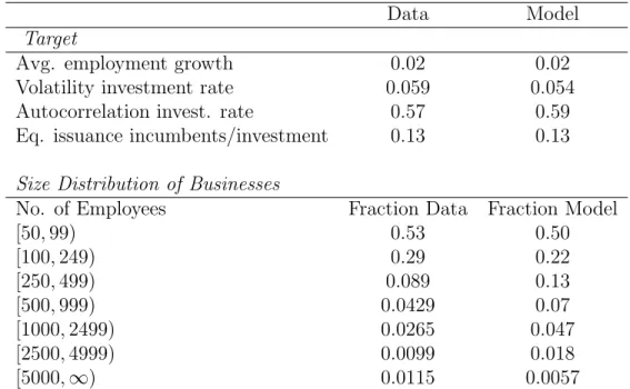
Table 1.2: Calibration Results

Data Model

Target

Avg. employment growth 0.02 0.02

Volatility investment rate 0.059 0.054

Autocorrelation invest. rate 0.57 0.59

Eq. issuance incumbents/investment 0.13 0.13 Size Distribution of Businesses

No. of Employees Fraction Data Fraction Model

[50,99) 0.53 0.50 [100,249) 0.29 0.22 [250,499) 0.089 0.13 [500,999) 0.0429 0.07 [1000,2499) 0.0265 0.047 [2500,4999) 0.0099 0.018 [5000,∞) 0.0115 0.0057

Targeted moments in the data, and their respective counterpart in the model. Data comes from Com-pustat, and BDS for the size distribution of businesses.

economy is 0.096, somewhat above the 0.086 value from the National Income Accounts. The model economy overstates the ratio of aggregate dividends to aggregate earnings in Compus-tat (0.45 versus 0.098). This also happens in the model byGourio and Miao (2010). Perhaps this should not be surprising since both model economies abstract from share repurchases, which is another way of dividend distribution. The model does a decent job in matching the ratio of aggregate equity issuance to aggregate investment in the data (0.15 versus 0.19). Moreover, the share of equity issuance by entrants relative to aggregate investment is 0.037 in the data and 0.067 in the model.20

Table 1.3: Non-targeted Moments

Variable Data Model

Investment rate 0.086 0.096

Dividends/Earnings 0.098 0.45

Agg. eq. issuance/ agg. investment 0.15 0.19 Eq issuance entrants/agg. investment 0.037 0.067

Non-targeted moments in the data, and their respective counterpart in the model. Data moments from Compustat.

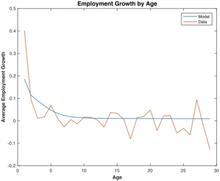
In Figure1.2, we plot age profiles of employment growth by firms21 _{in the model and}

the data. Although it is an untargeted moment, the model captures quite well the sharp decline in employment growth as firms age. In our model economy young firms are small and constrained, so they grow fast at the beginning. As they age and accumulate internal funds, they are likely to become less constrained and progressively reach their optimal size. As a result, the age-profile of employment growth of firms is expected to decrease with age. The fact that the baseline economy matches reasonably well the decline in the growth rate of employment with age suggests that the model is not exaggerating the impact of financial frictions on firm growth.

1.3.2

Aggregate effects of reforming the taxation of capital income

20_{To measure the share of equity issuance by new entrants and by incumbents in Compustat, we add up}

the equity issuance of all firms that report doing an IPO in that same year on one side, and the rest of the firms operating in that year on the other, and divide both by the sum of investment in capital expenditures of all firms.

21_{Unfortunately, age is not a variable available in Compustat, so we construct a proxy with the available}

Figure 1.2: Employment growth by age in the model and the data. 0 5 10 15 20 25 30 Age -0.2 -0.1 0 0.1 0.2 0.3 0.4 0.5

Average Employment Growth

Employment Growth by Age

Model Data

Average employment growth by age. Blue line is data generated from the model, orange line is data from Compustat, where age is computed in the as years since IPO (see AppendixB.1).

collects the same tax revenue as in the baseline economy22. The purpose of the proposed policy reform is twofold. Firstly, by equating the three tax rates, all forms of capital income are treated symmetrically from the household perspective. Secondly, by eliminating the corporate tax, financially constrained firms can accumulate profits and reach maturity (the dividend distribution stage) faster (in expectations).

We emphasize that the key insights from our simple model apply to the current stochas-tic model. Financial frictions imply that firms start their life constrained. For fixed produc-tivity, firms build internal equity over time, becoming less constrained and eventually start distributing dividends. Stochastic shocks imply that firms distributing dividends might be-come liquidity constrained again if their productivity grows sufficiently over time, so that the “life cycle process” is initiated again. By reducing the corporate tax and increasing the dividend tax, our proposed tax reforms intend to shift the tax burden from liquidity constrained firms (with high marginal valuation of capital) to firms distributing dividends (with low marginal valuation of capital). However, the effects of the reform are more in-volved than it seems at first sight. This is because firms react to higher dividend taxes by diminishing initial equity, raising the likelihood that firms become liquidity constrained, and

(partly) reversing the gains pursued with the elimination of corporate income taxation (see Section1.2.4)23_{. To minimize these effects, our proposed tax reform involves raising capital}

gains taxes together with dividend taxes. The rise in capital gains taxes encourages firms to issue more equity in order to minimize taxes paid on capital gains, (partly) undoing the distortions of dividend taxation on initial equity decisions (see discussion in Section1.2.4).

To check for potential non-linearities in the responses to tax changes, a tax reform that reduces the tax rate on corporate income to 0.21 is also considered. This experiment is also of interest since in 2017, the US corporate income tax rate was reduced to 0.21. To isolate the role of capital gains taxation from dividend taxation, we consider a tax reform that sets the corporate income tax rate to 0.21 while keeping the other tax rates at their value in the baseline economy. In this experiment, the dividend tax rate is raised to keep the government budget balanced. Finally, we consider a fourth tax reform in which the investment at entry is subsidized at the rate at which dividends are taxed. In order to evaluate the importance of entry for understanding tax responses, we also perform all the tax reforms in an economy in which entry is kept fixed at its value in the baseline economy24_.

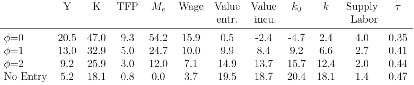
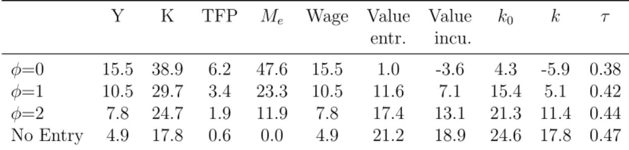
As further sensitivity analysis, AppendixD.1 considers economies in which the cost of entry rises proportionally (or more than proportionally) to the wage rate25. Appendix D.2 studies the sensitivity of the results when the representative household is allowed to choose labor hours (rather than being fixed as in the baseline economy).

Tax reform 1: Elimination of corporate income taxes

The results are shown on Table 1.4. The elimination of the corporate income taxes in the baseline economy (τc = 0.34) should be accompanied by an increase in capital income

taxes to 0.41 to keep government revenue constant (recall that in the baseline economy the dividend and capital gains tax was set to 0.15 and the interest income tax was set to 0.25). This revenue neutral tax reform leads to an increase in aggregate output of 12.2%, which is accompanied by a large increase in the aggregate capital stock (31.8%), in the number of firms (34.5%), and in aggregate TFP (4.6%). Note that the fact that aggregate capital and output rise less than the number of firms, indicates that both capital per firm and output per firm decrease (by 2% and 17%, respectively). Hence, the response of firm entry to the tax reform is crucial for the large increase in aggregate output and aggregate TFP in the

23 _{By financing a larger fraction of investments with internal funds, they reduce the cost of capital.} 24_{This is done by fixing the mass of firms to that of the baseline, and finding wages from the labor market}

clearing condition.

25_{The cost of entry depends on the wage rate: ce= ¯cew}φ_{, where the parameterφdetermines the elasticity}

of entry costs to wage changes. The baseline economy implicitly assumes φ= 0. Appendix D.1 considers alternative economies withφ= 1 andφ= 2.

Table 1.4: Effects of Tax Reforms

Y K TFP Me Wage Value Value k0 k τ

entr. incu. Tax Reform 1: τc = 0; financed by raisingτd=τg =τr

Baseline 12.2 31.8 4.6 34.5 12.2 1.2 -0.8 5.5 -2.1 0.41 No entry 3.7 15.4 0.0 0.0 3.7 16.3 15.6 19.3 15.4 0.48 Tax Reform 2: τc = 0.21; financed by raising τd=τg =τr

Baseline 6.0 14.8 2.3 16.4 6.0 0.3 -0.7 1.3 -1.4 0.26

No entry 1.9 7.5 0.0 0.0 1.9 7.5 7.7 6.3 7.5 0.31

Tax Reform 3: τc = 0.21; financed by raising τd

Baseline -1.2 10.0 -3.6 -19.1 -1.2 -1.9 5.0 -9.1 36.0 0.39 No entry 3.4 15.7 -0.4 0.0 3.4 -5.3 -2.1 -8.9 15.7 0.32 Tax Reform 4: τc = 0.21, financed by τd, including a subsidy to entry τ

Baseline 6.3 20.4 1.4 9.7 6.3 18.0 -6.1 137.3 9.8 0.29 No Entry 4.1 17.6 -0.2 0.0 4.1 20.0 -3.6 141.2 17.6 0.32

Percent changes from the baseline. From left to right: aggregate production (Y), aggregate capital (K), aggregate TFP (TFP), mass of entrants (Me), average value of entrants gross of initial equity payment (Value entr.), average value of incumbents (Value incu.), average capital at entry (k0) and average capital (k). In each experiment, we decrease corporate tax, but change other taxesτsuch that the government revenue is constant. τcorresponds to the value of the tax rate being changed, specified in each line.