Stephan Sauer:
Liquidity Risk and Monetary Policy
Munich Discussion Paper No. 2007-27
Department of Economics
University of Munich
Volkswirtschaftliche Fakultät
Ludwig-Maximilians-Universität München
Liquidity Risk and Monetary Policy
Stephan Sauer
∗Seminar for Macroeconomics
University of Munich
Germany
August 2007
Abstract
This paper provides a framework to analyse emergency liquidity assis-tance of central banks on financial markets in response to aggregate and idiosyncratic liquidity shocks. The model combines the microeconomic view of liquidity as the ability to sell assets quickly and at low costs and the macroeconomic view of liquidity as a medium of exchange that influences the aggregate price level of goods. The central bank faces a trade-off be-tween limiting the negative output effects of dramatic asset price declines and more inflation. Furthermore, the anticipation of central bank inter-vention causes a moral hazard effect with investors. This gives rise to the possibility of an optimal monetary policy under commitment.
Keywords: Liquidity shocks, Financial crises, Liquidity provision prin-ciple, Greenspan put, Optimal monetary policy intervention.
JEL classification: E58, E44, G18.
∗I would like to thank Gerhard Illing for fruitful discussions and Marco Sahm for helpful
com-ments. Address for correspondence: Seminar for Macroeconomics, University of Munich, Lud-wigstr. 28 RG, 80539 Munich, Germany. E-mail: [email protected].
1
Introduction
Liquidity is an important concept in finance and macroeconomics. The micro-economic literature in finance views liquidity roughly as the ability to sell as-sets quickly and costlessly. In macroeconomics, liquidity refers to a generally accepted medium of exchange or, in brief, money. Money is the most liquid asset due to the fact that it does not need to be converted into anything else in order to make purchases of real goods or other assets. This feature makes money valuable in both perspectives.
This paper uses this common perspective of money and links liquidity risk on an asset market with aggregate demand and aggregate supply on a goods market. Spillover effects from the asset market to the goods market can justify a central bank intervention on the asset market even if the central bank does not take the welfare of investors on the asset market into account. Hence, the model provides a framework to analyse the perceived insurance against severe financial turmoil by the Federal Reserve under Alan Greenspan, which has been termed the ‘Greenspan put’ in the popular press and ‘liquidity provision principle’ by Taylor (2005).
Liquidity provision has been studied in the literature with a focus on the role of financial intermediaries (see, e.g., Diamond and Dybvig, 1983; Allen and Gale, 1998; Diamond and Rajan, 2001, 2005; Goodhart and Illing, 2002). Considerably less research looked at liquidity provision by financial markets (see, e.g., Allen and Gale, 1994; Holmström and Tirole, 1998). Furthermore, all of these papers use models with real assets and claims. If the aim is to analyse optimal mon-etary interventions on financial markets, however, it seems to be natural that one has to use a model in nominal units, since the central bank can provide nominal fiat money but not real goods. Only recently, Gale (2005) and Dia-mond and Rajan (2006) have made first steps in that direction and developed models with nominal assets.1 Contributing to this literature, I develop an
ana-lytical framework based on the cash-in-the-market pricing model of Allen and Gale (1994, 2005) that directly links monetary policy and liquidity on financial markets.
Before I turn to the details of the model, the following two sections provide empirical and historical evidence of the role of liquidity on asset prices and in financial crises.
1Allen and Gale (1998) contains discussions about both monetary policy to limit some
ineffi-ciencies of bank runs and the effects of an asset market. Gale (2005, p. 2) himself, however, argues that this and more recent papers by Allen and Gale that use the same methodology are ‘essentially real (non-monetary) models’ and ‘focus on banks and banking, to the exclusion of other parts of the financial system.’
1.1
Empirical evidence for the role of liquidity on asset prices
One of the first studies that empirically links asset pricing and liquidity is Ami-hud and Mendelson (1986), who show that shares’ excess returns increase in the size of the average bid-ask spread, a well-known measure of an asset’s level of liquidity. Recent research has provided further important empirical ev-idence on the relevance of time-varying market-wide liquidity on asset pricing and of the effects of monetary expansions on liquidity during crisis periods. Pastor and Stambaugh (2003) measure market liquidity as the equally weighted average of individual shares’ expected return reversal. The authors start from the idea that a sell (buy) order should be accompanied by a negative (posi-tive) price impact that one expects to be partially reversed in the future if the share is not perfectly liquid. Sharp declines in this measure coincide with mar-ket declines and ‘flight to quality’ or ‘flight to liquidity’ episodes in which in-vestors want to shift from relatively illiquid medium to long-term assets such as shares into safe and liquid government bonds or cash. Examples of such incidents are discussed in the following section 1.2. Market-wide liquidity as measured by Pastor and Stambaugh (2003) appears to be a state variable that is important for share prices. Shares whose returns are more sensitive to aggre-gate liquidity have substantially higher expected returns, even as the authors control for exposures to the market, size and value factors of Fama and French (1993) and a momentum factor.
Acharya and Pedersen (2005) derive and estimate a liquidity-adjusted capital asset pricing model. In addition to the standard market beta, their model has three betas representing different forms of liquidity risk. One beta resembles the analysis in Pastor and Stambaugh (2003): Investors are willing to accept a lower expected return on an asset with a high return in times of market illiq-uidity. Futhermore, Acharya and Pedersen (2005) show that investors require a higher expected return for a security that becomes illiquid when the market in general becomes illiquid. Finally, investors require a lower expected return for an asset that is liquid if the market return is low. In the authors’ estimations, the last effect appears to have the strongest impact on expected returns. Most importantly for this paper, Chordia, Sarkar and Subrahmanyam (2005) establish an empirical link between the macro- and the micro-perspective of liquidity. The authors find that ‘money flows (...) account for part of the com-monality in stock and bond market liquidity.’ Furthermore, they use vector autoregressions to provide evidence that a loose monetary policy, measured as a decrease in net borrowed reserves or a negative interest rate surprise,2is
as-2Net borrowed reserves represent the difference between the amount of reserves banks need to
have to satisfy their reserve requirements and the amount which the Fed is willing to supply. A negative interest rate surprise is defined as a drop of the federal funds target rate below market
sociated with lower bid-ask spreads, i.e. increased liquidity, in times of crises.
1.2
Historical liquidity crises and central banks’ reactions
Besides these empirical studies, there is also a lot of anecdotal evidence how central banks reacted to liquidity crises, since the last decades have shown a number of such crises on financial markets. For example, Davis (1994) de-scribes five severe liquidity crises in international markets: The Penn Central Bankruptcy in 1970, the crisis in the floating-rate notes market in the UK in 1986, the failure of the US-High Yield bond market in 1989, the Swedish Com-mercial Paper crisis in 1990 and the collapse of the ECU bond market in 1992. Greenspan (2004) highlights three crises during his chairmanship at the Fed-eral Reserve (Fed), in which market participants wanted to convert illiquid medium to long-term assets into cash because they favoured safety and liquid-ity over uncertainty: The stock market crash in 1987, the LTCM-crisis 1998 and the terrorist attacks of September 11, 2001. This section provides a brief review of these three events and the central banks’, in particular the Fed’s, reactions to them. Sauer (2007) contains a more detailed discussion of the events.
On 19 October 1987 (‘Black Monday’), the Dow Jonex Index dropped by 22.6%. Many commentators blamed institutional investors that followed a portfolio insurance investment strategy for the dramatic crash in prices.3Similar to
stop-loss-orders, portfolio insurance implies automatic sell orders when the value of a portfolio or single shares falls below a certain threshold. If the absorption capacity of the market is limited, portfolio insurance can cause a vicious circle of price falls and further sell orders (see also section 4.3).
Grossman and Miller (1988) describe the events on 19 and 20 October against the background of their model in which market liquidity is determined by the demand and supply of immediacy, i.e. the willingness to trade immediately rather than to wait some time for a possibly better price. They argue that order imbalances were so great4that market makers became incapable of supplying
further immediacy. Market illiquidity materialised as delays in the execution and confirmation of trades and as the virtual impossibility of executing market sell orders at the quoted prices at the time of order entry.
As chairman of the Fed, Alan Greenspan managed to improve the confidence of investors and the liquidity of the market by issuing the following statement expectations (Chordia et al., 2005, pp. 112-113).
3For example, Gammill and Marsh (1988) report official statistics that show that institutional
investors who followed a portfolio insurance investment strategy were the heaviest net sellers on the New York Stock Exchange and in the S&P 500 index futures market.
4After a more than 10% decline of the Dow Jones between Wednesday, 14 October, and
Fri-day, 16 October, Gammill and Marsh (1988) note an ‘overhang of incomplete portfolio selling’ by portfolio insurers which caused additional selling pressure on the morning of Black Monday.
at 9am on 20 October 1987:
The Federal Reserve, consistent with its responsibilities as the Na-tion’s central bank, affirmed today its readiness to serve as a source of liquidity to support the economic and financial system (Greenspan, 1987).
The Dow Jones regained 5.9% and 10.1% on this and the following day, re-spectively. Garcia (1989) discusses the different tools the Fed used to limit the extent of the stock market crash. These included, besides communication via the quoted statement, mainly open market operations and the use of the dis-count window to provide liquidity in the form of additional money to the mar-ket. The handling of the crisis by Alan Greenspan, who was appointed as Fed Chairman only two months earlier, laid the foundations for the belief in an insurance against stock market losses, the alleged ‘Greenspan put’ (see also section 5.1).
In September 1998, the near-collapse of the hedge fund Long-term Capital Management (LTCM) caused severe turmoil on financial markets.5 After years
of extraodinary performance, LTCM experienced below-average returns in 1997 and even losses in the first half of 1998. In response, LTCM increased its lever-age, i.e. its debt/equity ratio, and focused even more on investments in rel-atively illiquid assets. The Russian default in August 1998 caused a flight to quality into liquid government bonds, while the prices of more illiquid assets fell dramatically. Margin calls forced LTCM to sell its assets into the falling market, which exacerbated the crisis. Other market participants could not (and some did not want to, see Brunnermeier and Pedersen, 2005) step in and buy assets, not least because they had copied LTCM’s trading strategies and were constrained in their available funds. LTCM’s supposedly sophisticated risk management system had not taken this endogeneity of risk sufficiently into account and its imminent collapse threatened the functioning of the Treasury bond market because of LTCM’s large short-positions on this market.
On 23 September, the New York Fed organised a private bailout of LTCM by 14 banks that had lent to the fund. In the following weeks, the Fed lowered its policy rate three times by 25 basis points in order to provide sufficient liquidity for financial markets. Both Greenspan (2004) and Meyer (2004), who was on the Fed’s Board of Governors at that time, admit that the purpose of these rate cuts was to calm financial markets rather than to stimulate the still expanding real economy. Indeed, the second cut boosted financial markets6and, for example,
5For a more detailed analysis of the LTCM-crisis, see e.g. IMF (1998), Jorion (2000) or Sauer
(2002).
6The cut was implemented between two scheduled meetings of the Federal Open Market
considerably lowered spreads on repos, swaps, corporate bonds and off-the-run treasuries, which all had increased dramatically after the Russian default (IMF, 1998, p. 39). Nevertheless, the Fed still feared the downside risks and lowered its policy rate a third time on 17 November despite lingering positive GDP data. Given the subsequent rise in inflation and equity prices until 2000, Meyer (2004, p. 121) later regretted this last cut.
The terrorist attacks in the morning of 11 September 2001 represented a very different form of a liquidity shock to financial markets. Liquidity evaporated from the financial system not because of margin calls, portfolio insurance strate-gies or a preference shock, but rather because large parts of the communication system and a lot of back offices in lower Manhattan were physically destroyed. One immediate response of the authorities was to leave the New York Stock Exchange, the American Stock Exchange and NASDAQ closed until 17 Sep-tember. Hence, liquidity problems concentrated in the payment and settle-ment system and did not affect the stock market immediately. In that sense, the effects were limited and the Fed could quickly withdraw the additional 108 billion US-$ in discount window credits, overnight repos and check floats it had supplied to banks until 13 September already by 20 September (Lacker, 2004, table 1).
In Europe, the European Central Bank (ECB) immediately issued the following press statement on 11 September:
After the unprecedented and tragic events in the United States today, the Eurosystem stands ready to support the normal functioning of the markets. In particular, the Eurosystem will provide liquidity to the markets, if need be. (ECB, 2001a)
Furthermore, the ECB conducted two one-day fine-tuning operations on 12 and 13 September with a volume of 69.3 and 40.5 billion Euro, respectively, in which all bids were satisfied. It also entered into a swap agreement with the Fed over 50 billion US-$ to provide dollar liquidity to European banks on 12 September (ECB, 2001b). However, the ECB left its key interest rates un-changed on its regular meeting on 13 September.
Just before U.S. stock markets reopened on the morning of Monday 17 Sep-tember, the Fed cut its target rate by 50 basis points. The ECB followed suit and also lowered its key interest rates by the same amount. The Fed contin-ued to cut rates on 2 October, 6 November and 11 December, while the ECB re-duced its rates only on 9 November. Although Lacker (2004, p. 961) argues that ‘the [Fed] interest rate cuts following September 11 are probably best viewed as addressing the medium- and longer-term macroeconomic consequences’ rather than a necessary response to disruptions in the payment system, the
contemporaneous action of central banks worldwide on 17 September7 hints
that this move was also aimed at rebuilding confidence and signalling that central banks would continue to provide liquidity if necessary. Indeed, on 17 September the Dow Jones opened only 3.2% below the closing value on 10 September. Until 21 September, the Dow lost 14.3% compared to 10 September, but regained quickly in the following weeks and reached the pre-terrorist level already in October.
A common feature of these crises is that the Fed lowered its interest rate to provide emergency liquidity to the market, although the mandate of the Fed in the Humphrey-Hawkins Act of 1978 focuses on price stability and full em-ployment. Taylor (1993) suggested a simple interest rate rule to capture these two goals:
it=rt∗+πt+ 0.5(πt−πt∗) + 0.5yt. (1)
The nominal interest rateitshould rise with the natural real rater∗t, inflationπt
relative to its target rateπ∗
t and the output gapyt. The comparison of the actual
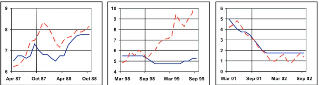
Fed funds target rate with the recommendation from this Taylor rule provides a simple test for the liquidity provision principle, i.e. a temporary departure of interest rates from the Taylor rule during financial crises (Taylor, 2005) in order to avoid negative spillover effects from the asset to the goods market. Figure 1 shows that the Fed decreased its policy rate in the months following all three crises as noted above. The Taylor rule, however, recommended a rise of the interest rate after the crises of 1987 and 1998. Therefore, monetary policy appears expansionary for about six months until April 1988 and even more so after the LTCM-crisis 1998. In contrast, the Taylor rate matches the actual Fed funds rate after the terrorist attacks in 2001 quite closely. From the beginning of 2002, actual monetary policy looks even restrictive compared to the Taylor rule.
Figure 2 reveals considerable differences in the development of inflation in the aftermath of the crises. For comparison, inflation is measured as the annual growth rate of both the consumer price index (CPI) and the personal consump-tion expenditure index (PCE), but the differences appear to be negligible. The average inflation rate one and a half to two years after the crises compared to average inflation in the six months up to the crises increased by 0.8 percentage points after 1987 and 1.7 points after 1998.8 In contrast, inflation decreased by
0.4 (PCE) or 0.9 (CPI) points after 2001. Therefore, expansionary monetary pol-icy via the liquidity provision principle appears to have contributed to price
7Besides the Fed and the ECB, also the Bank of England, the Swedish Riksbank, the Bank of
Canada and other central banks worldwide lowered their policy rates on the same day.
8Besides the rise in consumer prices, expansionary monetary policy may also have contributed
Figure 1:Federal funds target rate (solid line) and Taylor rule rate (dashed line) in the U.S. during the crises in 1987, 1998 and 2001.
Notes: The Taylor rule rate is based on equation (1) withπtmeasured as the annual growth rate
of the consumer price index andyt measured as the quarterly OECD-output gap transformed
into monthly data with a cubic spline. The Taylor rate is adjusted for time-varyingr∗
t andπt∗by
matching the average Taylor rate in the six months prior to the respective crisis with the average Federal funds target rate over this period. Data source: Thomson Financial Datastream.
Figure 2: CPI (solid line) and PCE (dashed line) inflation rates in the U.S. after the crises in 1987, 1998 and 2001.
Notes: Inflation is measured as the annual growth rate of the consumer price index (CPI) and the personal consumption expenditure index (PCE). Data source: Thomson Financial Datastream. increases after 1987 and 1998, while a normal or even restrictive stance of mon-etary policy added to a decline of inflation after 2001.
All three historical episodes of liquidity crises demonstrate that central banks, and in particular the Fed under Alan Greenspan, stood ready to provide liq-uidity in times of financial crises. Greenspan (2004, p. 38) states that the ‘im-mediate response on the part of the central bank to such financial implosions must be to inject large quantities of liquidity,’ in line with the traditional Bage-hot (1873) principle for a lender of last resort activity to ‘lend freely at a high rate against good collateral.’ But the events also indicate that not all financial crises are alike and central banks face a difficult task to decide on the optimal policy, which depends on the associated cost and benefits. The rest of this pa-per develops a stylised model of an asset market and a goods market which provides a framework to analyse the relevant trade-offs for the central bank.
1.3
The model in a nutshell
The model consists of two separate markets, an asset market and a goods mar-ket. The main focus is on developments on the asset market, but these de-velopments have important implications for the goods market. Although the monetary authority only cares about deviations of goods prices and quantities from the optimal values, the spillover effects from the asset market may require a central bank intervention on this market.
In the model, investors can invest on an asset market in liquid money and potentially illiquid, but productive assets, called shares, in order to optimally satisfy their uncertain consumption needs on the goods market over two peri-ods. Two channels link the goods market to the asset market: First, the amount of money held by investors determines together with the size of a liquidity shock the aggregate demand of investors on the goods market which is subject to a cash-in-advance constraint. Second, a dramatic decrease of the asset price negatively influences the goods supply in the final period because it forces in-vestors to costly liquidate their asset. Hence, the central bank faces a trade-off between inflating a demand shock today, which causes higher losses today, and limiting a negative supply shock tomorrow, which will cause higher losses to-morrow. Expectations of central bank intervention give rise to a moral hazard effect with additional investment in less liquid, but productive shares. If the central bank has the possibility to commit to some future policy, it should opti-mally weight these productivity gains against the expected intervention costs. Section 2 analyses the basic model under certainty and aggregate risk. Section 3 provides further insights into the trade-off the central bank faces and derives the optimal central bank intervention before section 4 discusses the impact of idiosyncratic risk. After the discussion of the related literature in section 5, section 6 concludes.
2
Model
2.1
Framework
A continuum of ex ante identical investorsiis uniformally distributed on an intervallI = [0; 1]. They can invest on an asset market and buy goods for
consumption on a separate goods market. An investoriderives utility from consumptionctin periodst= 1,2according to the utility function
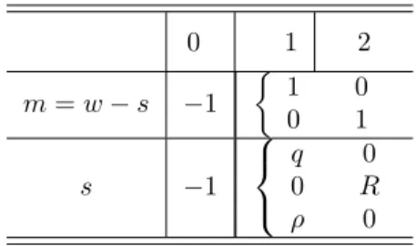
Table 1:Payoffs of money and shares int= 0,1,2. 0 1 2 m=w−s −1 1 0 0 1 s −1 q 0 0 R ρ 0
γζirepresents a liquidity shock that consists of an aggregate liquidity shockγ
and an individual liquidity shockζi. The distribution functions of both shocks
are assumed to be uncorrelated, symmetric, having a positive support and an expected value of 1 int= 0, i.e.E0[γζi] =
R∞
−∞γf(γ)dγ·
R∞
−∞ζif(ζi)dζi= 1.
Every investor is endowed with nominal wealthwthat can be invested int= 0
in nominal moneymand a real assets, called shares, on a primary market with priceq0= 1fixed andsendogenous. The asset pays a fixed nominal returnR
int= 2and can be traded at the nominal priceqon a secondary asset market in
t= 1after the realisation of the liquidity shockγζi, but before goods are traded
on the goods market. Besides, investors have access to a costly real liquidation technique, which transformszunits of the assetsintoρz units of additional consumption goods in period 1 withρ <1. The individual cost of liquidation
is the missed nominal returnRz int = 2and the social cost is a reduction of aggregate supply int = 2by∆(z).9 The assetscan also be interpreted as a
nominal bond with a fixed interest rateRand a real put option with a strike price ofρ. Table 1 summarises the payoffs ofmandsint= 0,1,2.
At the beginning oft = 1 and2, homogenous, infinitely divisible and
non-storable consumption goods are produced with capital and labour input from workers who can participate only on the goods market and receive a nominal wageψtthat is determined att−1.10 These goods must be bought by investors
and workers with money, i.e. they are subject to a cash-in-advance constraint. The price of consumption goodsptis determined by demand for goods from
workers and investors and the aggregate supply of goods. Markets are
com-9For example, Shleifer and Vishny (1992) and Allen and Gale (1998) contain a discussion of the
costs of premature liquidation of assets. The costly liquidation technology shall represent investors possibility to a) partly liquidate their capital, b) sell their capital to less productive owners or c) cut down replacement investments because firms’ refinancing possibilities depend on their share price as in the financial accelerator model by Bernanke, Gertler and Gilchrist (1999). In this model, the assumptionρ <1guarantees that money is not fully dominated by the asset given the price determination on the goods market as explained in section 2.2.2 and the absence of central bank interventions. For the corresponding condition with central bank intervention, see Corollary 2 on page 29.
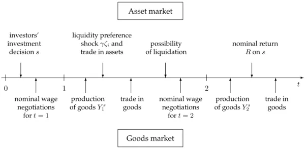
-t Goods market Asset market 0 ? investors’ investment decisions 6 nominal wage negotiations fort= 1 1 6 production of goodsY1s ? liquidity preference shockγζiand trade in assets 6 trade in goods ? possibility of liquidation 6 nominal wage negotiations fort= 2 2 6 production of goodsY2s ? nominal return Rons 6 trade in goods
Figure 3:Time structure of the model.
petitive but incomplete. Figure 3 summarises the timing of the model.
2.2
Under Certainty
2.2.1 Investors’ problem and asset market
Before I analyse the effects of liquidity shocks γζi, I solve the model under
certainty, i.e.γ=ζi= 1. The individual investor maximises her utility function
(2) subject to her budget constraint and her cash-in-advance constraint (CIA) in
t= 1.11 She controls her initial investment in the assets, her consumptionc
tin
t= 1and2bought on the goods market with cash, her demand for additional assets int = 1,ˆs, and the extent of costly liquidationz, which is subject to a
non-negativity constraint:12 max s,c1,c2,s,zˆ U(c′ 1, c2) = ln (c1+ρz) +βlnc2 s.t. (3) p1c1+p2c2≤w−s+Rs+ (R−q)ˆs−Rz p1c1+qsˆ≤w−s 0≤z≤s
11The budget constraint implicitly includes the CIA fort= 2as the investor holds only cash
when she enters the goods market int= 2.
12The Cobb-Douglas utility function (2) makesc
Note that an investors’ total consumption int = 1,c′
1, is the sum of the
con-sumption purchased via the goods market, c1, and the real return from the
possible liquidation of assets,ρz. Solving the maximisation problem with the Lagrangian max s,c1,c2,ˆs,z Λ = ln (c1+ρz) +βlnc2 −λ[p1c1+p2c2−(w−s)−Rs−(R−q)ˆs] −µ[p1c1+qsˆ−(w−s)]
yields as first-order conditions
dΛ dc1 = 1 c1+ρz −λp1−µp1= 0 −→ µ+λ= 1 p1(c1+ρz) (4a) dΛ dc2 = β c2 −λp2= 0 −→ λ= β p2c2 (4b) dΛ ds =−λ+λR−µ= 0 −→ µ=λ(R−1) (4c) dΛ dsˆ =λ(R−q)−µq= 0 −→ µ=λ R q −1 (4d) dΛ dz = 1 c1+ρz ρ−λR≤0 (4e) dΛ dλ =−p1c1−p2c2+ (w−s) +Rs+(R−q)ˆs≥0 (4f) dΛ dµ =−p1c1−qˆs+ (w−s)≥0 (4g) and dL dzz= 0, dL dλλ= 0and dL
dµµ= 0as complementary slackness conditions.
13
Since the costly liquidation is inefficient forp1ρ < 1, investors will not use
it under certainty, and z = 0.14 As will become clear from the discussion of
the goods market in the next section, the price of goodsp1equals its expected
value, i.e.p1= 1, under certainty, soρ <1is a necessary and sufficient
condi-tion forz= 0.
(4c) and (4d) show thatq= 1in the equilibrium under certainty because
hold-ing money would be dominated fromt= 0tot= 1forq >1ands=w, while holding shares would be dominated fromt = 0tot = 1forq <1ands= 0. Forq = 1, money and shares are equivalent assets fromt = 0tot = 1. Since money is dominated by shares over the long run, the CIA is binding int= 1.15
13The second-order conditions for a maximum are fulfilled, since (3) maximises a strictly concave
utility function under linear constraints and the optimum is an interior solution.
14By pluggingµfrom (4c) in (4a), solving forλand then pluggingλin the inequality (4e), it can
be shown thatdΛ/dzis negative and thusz= 0as long asp1ρ <1.
15SinceR >1by assumption andλ >0from (4b), the FOC for optimal investment insyields
The only possible symmetric equilibrium isˆs= 0, i.e. there is no trade on the
asset market int = 1, and money is only held for consumption int = 1: (4g) reduces top1c1=w−s. The combination of (4a) and (4b) shows that a binding
CIA drives a wedgeµ, the marginal utility of cash’s liquidity services, between
the marginal utilities of consumption int= 1andt= 2:16 µ+ β
p2c2
= 1
p1c1
.
According to (4c), the wedgeµequals the marginal utility of wealth,λ, times the excess return of shares over money,R−1, such that the marginal rate of
intertemporal substitution equals the price ratio times the return on shares:
c2
βc1 = p1
p2
R.
Given the optimal consumption int= 1and2, the budget constraint (4f) and the CIA (4g), the optimal investment decision int= 0is
s= β
1 +βw and
m= 1 1 +βw.
An individual investor has consumption demands of17 c1= w (1 +β)p1 and c2= βRw (1 +β)p2 .
Finally, the investment and consumption decisions of individual investorsican be aggregated to aggregate investment and consumption. Let capital letters denote aggregate values of the respective variable, i.e. W ≡ Ri∈Iwdi,M ≡ R i∈Imdi,S ≡ R i∈Isdi,C1 ≡ R i∈Ic1diandC2 ≡ R i∈Ic2di. GivenI= [0; 1], the
following Proposition 1 summarises the situation under certainty:
Proposition 1 In the symmetric equilibrium under certainty, investors split their wealth in moneyM = 1+1βWand sharesS= 1+ββWand consumeC1= p1(1+1 β)W
andC2= p2(1+βRβ)W. The asset priceq= 1and no assets are traded in the symmetric
equilibrium.
PluggingR= 1/βinto the results of Proposition 1 yields a special result:
16Note thatµ≥0represents the standard complementary slackness condition: If the CIA is not
binding (µ= 0), the marginal utility of money’s liquidity services is zero; but if the marginal utility of money’s liquidity services is positive, the liquidity constraint becomes binding (µ >0).
17For completeness, the Lagrangian parameters areλ=1+β
Corollary 1 If the interest rateRequals the discount rate1/β, investors spend the same amount of money in both periods, i.e. p1C1 = p2C2, and consume the same
amount of goods, i.e.C1=C2, if prices remain constant.
To concentrate on the intertemporal substitution effects of liquidity prefer-ence shocks, I start from the situation in Corollary 1 with perfect consumption smoothing and thus assumeβR= 1where useful below.
2.2.2 Goods production and goods market
Because I want to focus on events on the asset market, in particular on the effects of emergency liquidity provision by the central bank in section 3, and the direct spillover effects to the goods market, the model includes a very styl-ised version of a goods market. Non-storable goods are produced by a mass of 1 of identical competitive firms at the beginning of periods t = 1,2 with total labour inputNt = ¯N from identical workers who cannot participate on
the asset market and capital inputKtaccording to a Cobb-Douglas production
function
Yt=KtαN¯1−α (5)
with 0 < α < 1. Trade on the goods market takes place after the realisation of the liquidity shock for investors and after trade on the asset market. While aggregate supply is already produced and thus fixed atYt, aggregate demand
consists of demand from workers based on their nominal labour incomeψtand
from investors as derived in the previous section.
Given a Cobb-Douglas production function with constant returns to scale and perfect competition, the Euler theorem states that production factors are paid their marginal product times the respective factor input. With the production function (5), workers should receive the share of total outputYt that reflects
their relative importance in production as captured by 1−α, while capital owners should receiveαYt. Furthermore, I assume that investors’ demandCt
represents the whole factor income of capital, such thatCt=αYtand that the
real investmentSdetermines the constant producible aggregate real supplyY¯
with∂Y /∂K¯ ·dK/dS >0.18
Since I have a model in nominal units, labour income for periodt is deter-mined in nominal wage negotiations between workers and firms19 at the end
of periodt−1such that their expected real income isΨt= (1−α)Yt. Hence,
the agreed nominal wage is ψt = ΨtEt−1[pt] = (1−α)YtEt−1[pt] given the 18Although this is an obvious departure from a full general equilibrium model where the income
from capital is directly linked to the marginal product of capital, the crucial effects of the model should still hold in general equilibrium under the assumption of a cash-in-advance constraint for investors and limited asset market participation.
expected price levelEt−1[pt]. E0[p1]is normalised to 1.20 For simplicity, I
as-sume that workers build their price expectations based on the quantity equa-tion, i.e. they expect that investors use all their available nominal funds for the purchase of consumption goods in the respective period.21 Hence, money
holdingsM =W−S=E0[p1C1]and the supply of goodsY¯ represent the
in-formation set for the wage negotiations int = 0. The nominal return from the
investmentRSplus any unusedM fromt= 1equalE1[p2C2]. Together with
Ys
2, this provides the information for the negotiations int = 1. The expected
nominal demand Et−1[ptCt]in turn has to be equal to the expected income
share of capital,Et−1[pt]αYt. Due to the normalisationE0[p1] = 1,C1=αY¯.22
Under certainty, this also means thatE1[p2] = p2 = 1as well if βR = 1
be-cause the CIA binds (µ >0) and investors transfer no money tot = 2. Hence, investors’ nominal funds are thus identical int= 1and2. IfβR6= 1, investors’
nominal funds differ in both periods under certainty. The nominal wage nego-tiations int= 1determineψ2such that the pricep2adjusts such that workers
receive1−αand investors αof the constant aggregate supplyY¯ int = 2.
Hence, aggregate demandYd
t and aggregate supplyYtsare
Yd t = ψt pt +Ct= Ψt+Ct and (6) Yts= ¯Y . (7)
To summarise the equilibrium on the goods market under certainty forβR= 1, the expected price of goodsEt−1[pt]equals the actual pricept= 1fort= 1,2.
Investors consumeC1 =C2=W/(1 +β), while total production equalsY1=
Y2 =W/[α(1 +β)]and workers consume 1−αα times investors’ consumption,
i.e.Ψ1= Ψ2=1−ααW/(1 +β).
2.3
Aggregate Risk
What is the efficient response to a positive aggregate demand shock in t = 1? If the supply of goods can be adjusted to the increased demand, it will be increased until the marginal costs of doing so equal the marginal benefit. In this model, production takes place before the shock, so the liquidation technology offers the only way to increase supply int = 1. Since the liquidation costs are very high, investors will use it only for large shocks. In an intermediate range, prices adjust such that the marginal rate of intertemporal substitution equals
20This assumption avoids any problems with a possible indeterminacy of the price level. 21For example, Illing (1997) and Walsh (2003) model aggregate demand with a quantity equation. 22Actually,C1is determined byW,Sandp1(see table 2). With nominalWand realC1 =αY
fixed, p1 is no free parameter any more. But the link betweenSandKand thusY¯ could be
the relative prices.
Since the optimal investment strategy int= 0depends on expectations about developments on the asset and the goods market int = 1and 2, the model has to be solved by backward induction. Hence, the allocations on the goods market int= 2andt= 1as well as the influence of the shocks on the optimal behaviour of investors on the asset market int = 1have to be taken into
ac-count when one solves the utility maximisation problem of investors int= 0. For illustrative purposes, however, it will be easier to begin with the descrip-tion of the asset market, turn to the goods market afterwards and then solve the initial investment problem given the behaviour int= 1,2.
2.3.1 Asset market
The optimal investment decision problem for an individual investor under ag-gregate risk becomes
max s,c1,c2,s,zˆ E[U(c′ 1, c2)] = Z ∞ −∞ (γln (c1+ρz) +βlnc2)f(γ)dγ s.t. (8) p1c1+p2c2≤w−s+Rs+ (R−q)ˆs−Rz p1c1+qˆs≤w−s 0≤z≤s.
The solution to this maximisation problem in section A of the appendix uses the Leibniz-Rule and yields as first order conditions
∂Λ ∂c1 = γ c1+ρz −λp1−µp1= 0 (9a) ∂Λ ∂c2 = β c2 −λp2= 0 (9b) ∂Λ ∂ˆs =λ(R−q)−µq= 0 (9c) ∂Λ ∂z = γ c1+ρz ρ−λR≤0 (9d) ∂Λ ∂λ =−p1c1−p2c2+w+ (R−1)s+ (R−q)ˆs−Rz≥0 (9e) ∂Λ ∂µ =−p1c1−qˆs+w−s≥0 (9f) dΛ ds = Z ∞ −∞ [λ(R−1)−µ]f(γ)dγ= 0. (9g) and ∂Λ ∂zz= 0, ∂Λ ∂λλ= 0and ∂Λ
∂µµ= 0as complementary slackness conditions.
23
23As for the maximisation problem (3) under certainty, the second-order conditions for a
Since all investors are identical without idiosyncratic risk, they all want to sell or buy assets in response to an aggregate liquidity shockγ at the same time in t = 1 in order to adjust their money holdings optimally to their desired consumption which is subject to the CIA. As the aggregate stock of assets is determined int= 0, however, they cannot sell or buy in the aggregate. Hence, the asset priceqhas to adjust to exclude any excess demand or supply of assets,
i.e. market clearing int= 1requires thatSˆ=R
i∈Isdiˆ = 0.
Depending on the realisation of the liquidity shock γ, the asset priceq, the Lagrangian parametersλandµand the choice variablesc1, c2andzlie in three
different ranges. Forγ < β(W−S)
RS ≡ CIA, investors want to transfer wealth
into the next period. This drives up the asset priceq, which is bounded byR:
Nobody would be willing to pay more for the asset than the asset’s fixed payoff in the next period. In this case, the CIA becomes non-binding (µ= 0).
For greater values ofγ, however, the CIA is binding and the asset price de-pends on the cash in the market as in Allen and Gale (1994, 2005). As long as investors do not liquidate their assets, the asset price captures the full effect of
γ ∈hβ(W−S)
RS ;
β(W−S)
p1ρS
i
. For sufficiently large liquidity shocksγ > β(W−S)
p1ρS ≡
LIQ, the asset priceq falls to a level where the investors become indifferent
between liquidating the asset and selling the asset. Since they cannot sell in the aggregate, they costly liquidate part of their assets (z > 0). Table 2 sum-marises the equilibrium values of the relevant variables in the three ranges of
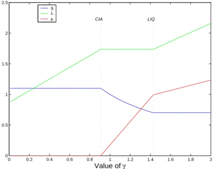
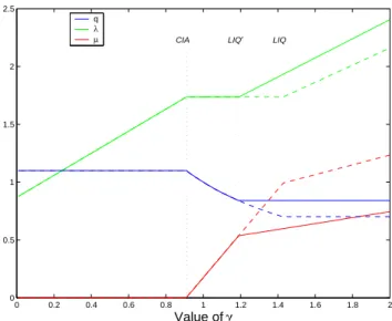
γ.24Figure 4 illustrates the asset priceqand the two Lagrangian parameters on
the budget constraint and the CIA as a function ofγforR = 1/β = 1.1, W = 1, S= 1+ββW, ρ= 0.7. The possibility of a severe drop inqcaptures the micro-economic view of liquidity, as an illiquid asset cannot be sold quickly without costs.
Turning to the optimal investment decision int = 0, the first-order condition for optimal investment in the asset is given by equation (9g). Using the re-sults forλandµfrom table 2 and the definitions of the cumulative distribu-tion funcdistribu-tionF(x) ≡ R−∞x f(γ)dγ of the liquidity shockγ and the function G(x)≡Rx
−∞γf(γ)dγ, section A in the appendix shows that the determination
of the optimal investmentsrequires an explicit parameterisation of the shock’s density functionf(γ). I assumeγto be uniformly distributed betweenaand
bwith0 < a < b. Table 3 summarises the information which is derived in the appendix.
There is only one variable left that depends on the realisation ofγ, namely the and the optimum is an interior solution.
24Note that the Cobb-Douglas preferences (2) determine the relative expendituresp
1c1top2c2
such thatc1is independent fromp2andc2is independent fromp1in general. Only forγ > LIQ
and thusz > 0,c2 depends onp1ρbecause this is the nominal value of liquidation int= 1.
Table 2:Summary of the values of the asset priceq, the Lagrangian parametersλand
µand the choice variablesc1, c2andzafter the realisation ofγint= 1.
γ < β(W−S) RS ≡CIA β(W−S) RS ≤γ≤ β(W−S) p1ρS γ > β(W−S) p1ρS ≡LIQ q R β(W−S) γS p1ρ λ w−βs++γRs β(W−S+RS) RS(w−s+Rs) p1ρ(β+γ) R(w−s+p1ρs) µ 0 λβ(γRSW −S)−1 λ R p1ρ−1 z 0 0 γp1ρs−β(w−s) p1ρ(β+γ) c1 p1(βγ+γ)(w−s+Rs) wp−1s wp−1s c2 p2(ββ+γ)(w−s+Rs) Rsp2 βR(w−s+p1ρs) p2p1ρ(β+γ) 0 0.2 0.4 0.6 0.8 1 1.2 1.4 1.6 1.8 2 0 0.5 1 1.5 2 2.5 Value of γ CIA LIQ q λ µ
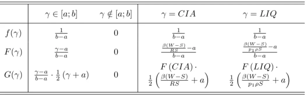
Table 3:Summary off(γ), F(γ), G(γ)int= 1. γ∈[a;b] γ /∈[a;b] γ=CIA γ=LIQ f(γ) b−1a 0 b−1a b−1a F(γ) γ−a b−a 0 β(W−S) RS −a b−a β(W−S) p1ρS −a b−a G(γ) γ−a b−a · 1 2(γ+a) 0 F(CIA)· 1 2 β(W−S) RS +a F(LIQ)· 1 2 β(W−S) p1ρS +a
goods pricep1, which is determined on the goods market as described in the
following section. As noted above, however, the utility function (2) implies thatp1 only matters forλ, µ, Ctin the rangeγ ≥ β(pW1ρS−S). Table 2 shows that
in this range investors use all their nominal fundsw−sto buy consumption goods on the goods market. The detailed description of the goods market in the next section 2.3.2 shows thatp1 = 1in this case. Given this information,
one can now solve for the optimal investment in the assets.
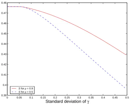
Figure 5 illustrates that the optimal investment is decreasing in the standard deviation ofγ,σ(γ) = b−a
2√3, while this effect is more pronounced for a lower
real payoff of the liquidation technologyρ. Without aggregate risk,
proposi-tion 1 states that investors holdS = 1+ββW ≈0.4762forR = 1/β = 1.1and
W = 1. Initially, introducing aggregate risk does not affectSbecause the asset
priceqabsorbs the full impact of the liquidity shock for the chosen parameter values, i.e. the CIA always binds (F(CIA) = 0) and no assets are liquidated (F(LIQ) = 1) given the equilibriumS. Further increasingσ(γ)makes the
risk-averse investors reduce their investmentS. As the real payoff of liquida-tions Z increases in ρand the liquidation thresholdLIQdecreases in S, the
reduction inScaused by increased aggregate risk is dampened by a greaterρ
and the solid line (ρ= 0.9) lies above the dashed line (ρ= 0.5) in figure 5. This is the solution of the model with aggregate risk and access to a costly real liquidation technology for investors. The analysis of an emergency liquidity assistance by the central bank requires at first a deeper discussion of the goods market in the next section. Furthermore, the costs and benefits of such an inter-vention need to be based on an explicit welfare function for the central bank. I turn to this issue in section 3.
0 0.05 0.1 0.15 0.2 0.25 0.3 0.35 0.4 0.45 0.5 0.39 0.4 0.41 0.42 0.43 0.44 0.45 0.46 0.47 0.48 Standard deviation of γ S for ρ = 0.9 S for ρ = 0.5
Figure 5:Optimal investmentSforR= 1/β= 1.1andW = 1.
2.3.2 Goods market
Investors’ liquidity shocks int = 1can spill over to the goods market via a demand effect in t = 1and a supply effect in t = 2. Letη denote the first
channel that links the asset market and the goods market: For small realisations of the liquidity shockγ < CIA, the CIA of investors becomes non-binding and they do not use all their money for consumption int = 1. This represents a negative nominal aggregate demand shock on the goods market, represented byη <0. If the liquidity shockγis in the range ofCIA≤γ≤LIQ, the asset
priceq absorbs the full effect of the liquidity shock as noted in the previous section and investors’ nominal demandp1C1 = W −S. For large liquidity
shocksγ > LIQ, investors liquidate part of their assets and thus increase the total resources available for consumption int = 1beyondY¯. Since investors
satisfyρZof their desired consumption goods with the liquidation technology,
they still demandp1C1=W −Son the goods market. If, however, the central
bank intervenes on the asset market and injects additional money in case of large realisations ofγ as will be shown in the following section 3, investors’ nominal demand rises above the level expected in the wage negotiations. This is represented by a positive aggregate demand shockη >0.
The rest of aggregate demand depends on nominal labour incomeψt, which is
Perfect competition and the Cobb-Douglas production function (5) require that workers can consume (1−α)Yt in t given the expected price level Et−1[pt]
which is normalised to 1 fort= 1. Workers build their price expectations based on the quantity equation, i.e. they expect that the total amount of money held by investors at the time of the wage negotiations is spent int= 1. Hence, the expected nominal demandE0[p1C1] =W −Shas to be equal to the expected
capitalists’ income share E0[p1]αYt = αY¯ as E0[p1] = 1.25 Therefore, the
aggregate demand relationship from equation (6) becomes
Yd
1 =
ψ1+W −S+η
p1
, (10)
while aggregate supply is again fixed to26 Ys
1 = ¯Y .
Note that the price impact of nominal demand shocksηoriginating from the
asset market is less than 1 asψ1is constant. Hence, the first channel that links
the asset with the goods market,η, causes a redistribution effect from investors’ consumption share atp1= 1towards workers forη < 0and from workers
to-wards investors forη >0. Given the determination ofE0[p1]described above,
positive price shocks can only occur with additional money from the central bank which will be discussed extensively in the following section 3.
The exercise of the real put option acquired with the assets, i.e. the applica-tion of the costly liquidaapplica-tion technique, in response to large liquidity shocks
γ > LIQwith no or insufficient emergency liquidity assistance by the central bank causes the second link between the asset market and the goods market: Without costly liquidations, the capital stockKtis fixed over the time horizon
of this model and aggregate output isY¯, given the initial investmentS. If
in-vestors choose to liquidate part of their shares, i.e.Z >0, this liquidation takes place after production int = 1and increases the real resources available for consumption int= 1, but reducesK2.The lower capital input int= 2lowers
25This assumption is a short-cut from the rationalErat
0 [p1C1]because investors will spend all
their money int= 1only as long as their CIA binds, i.e.γ≥CIA, and less forγ < CIA. This impliesErat
0 [C1]< C1(γ≥CIA)andE0[η] < 0without central bank intervention. Hence,
workers get more than their expected share of aggregate supplyY¯ int= 1on average and are
thus implicitly compensated for their real income risk int= 1. To summarise, the way workers form their expectations and the normalisation ofE0[p1]determine the size of the redistribution
effect of investors’ nominal demand on workers after the realisation ofγ, but not the possibility of such redistributions.
26Y¯may be different from the one under certainty, however, since it depends onSwhich may
¯
Y by∆ (Z), withddZ∆>0, and aggregate supply becomes
Y2s= ¯Y −∆(Z). (11)
Any risk has disappeared from the model at the time of the nominal wage ne-gotiations fort = 2. Workers build their price expectationsE1[p2]based on
investors’ safe nominal revenuesR(S−Z), potentially unused money
hold-ings W −S −p1C1 and the known Y2s. Again, perfect competition allows
them to consume Ψ2 = (1−α)Y2, which implies a nominal wage of ψ2 =
E1[p2] (1−α)Y2.27 The aggregate demand equation fort= 2then is
Y2d =
ψ2+R(S−Z) +W −S−p1C1
p2
. (12)
and equals aggregate supply atp2=E1[p2]in equilibrium: Ψ2+C2= ¯Y −∆(Z).
p2 and its expected value adjust relative to p1 such that investors’ real
con-sumption C2 = α ¯
Y −∆(Z). For example, if investors’ liquidity shock γ
is within the intermediate range CIA < γ < LIQ, the CIA is binding and W −S=p1C1, but no assets are liquidated, i.e.Z= 0. (12) reduces to
Yd
2 =
ψ2+RS
p2
andp2 =p1 = 1forβR= 1and a sufficiently small variance ofγthat leaves
S =β/(1 +β)W from the certainty case unaffected (see also figure 5). Since
investors’ Cobb-Douglas-preferences smooth nominal expenditures overt= 1
and 2,p2has no effect on investors’ behaviour int= 1givenS.
To summarise, the two direct channels that link the asset market to the goods market in this model are the aggregate demand shock η in period 1 and the aggregate supply shock∆in period 2, which both depend on the realisation of
the liquidity shockγint= 1.
27Note again that investors do not react to possible changes ofp2relative to a constantp1because
the Cobb-Douglas-preferences determine the expenditure share rather than real consumption in each period. Hence, given the constant produceable aggregate supplyY¯ and workers’ desired
income of(1−α)Y2,p2would have to deviate fromp1even ifγ =E0[γ] = 1for example if βR6= 1in order to equate investors’ intertemporal rate of substitution to the relative pricep1/p2
3
Central bank intervention
3.1
Welfare function
The direct spillover effects from the asset market to the goods market mean that the central bank may intervene on the asset market even if it does not take investors’ welfare into account. The loss functionLof the central bank consists of the weighted sum of two parts: The increase ofp1 above the desired price
levelp∗
1because of the associated real income loss of workers and the deviation
of aggregate supplyYs
2 fromY¯ caused by liquidationsZ,∆ (Z):28 L= (p1−p∗1)−ω Y2s−Y¯
. (13)
ω reflects the weight on the real income loss of workers in t = 2 relative to
the weight on the real income loss of workers int = 1caused by a rise inp1
and thus implicitly includes the central bank’s time discount factor. Letp∗
1be
normalised to1and thus equal the expected price levelE0[p1]. It is sufficient
to concentrate on p1 and Y2s in this stylised model becauseY1s is produced
before any shocks occur and thus not directly influencable by monetary policy under discretion29 and nominal wage negotiations fort = 2 take place after
any shocks and determinep2such that workers receiveΨt= (1−α)Y2s.
The concentration on goods markets can be justified with several arguments: From a positive perspective because price stability and - differently accentu-ated - output stability are the mandate of most central banks in the world, where price stability is generally interpreted as a low but positive growth rate of some form of a consumer price index. From a political economy perspective, since people living mainly from their nominal labour income represent the ma-jority of voters in a society and, as I show in this paper, this focus may even improve the welfare of investors as well. Finally, also from a normative per-spective within the New Keynesian framework as argued by Woodford (2003) because asset prices are in general a lot more flexible than goods prices and the monetary authority should focus on a measure of relatively sticky core infla-tion to limit the distorinfla-tions caused by nominal rigidities.30
28The discussion below shows that the central bank cannot intervene symmetrically in this
model. Hence, the linear loss function represents a useful simplification. The results of the model are robust to a loss function that is quadratic in inflation and output deviations from their re-spective targets, but the comparative static analysis and the restrictions on some parameter values become more complex (see section B in the appendix).
29The indirect effect of central bank intervention on aggregate supply will be analysed in section
3.5. Section 3.6 discusses how optimal monetary policy can take the indirect effect into account.
30Note, however, that the normative argument has been subject of a long discussion in
macroeco-nomics that goes far beyond the scope of this paper. For example, Woodford’s argument neglects the information content of asset prices about future consumer price inflation that was emphasised by Alchian and Klein (1973). These authors concluded that asset prices should receive a very high
3.2
Asset market
The central bank has the possibility to prevent the costly liquidation of shares if it acts as a lender or rather liquidity provider of last resort to the financial market. That means, it can enter repurchasing agreements with investors at a price (just) high enough to prevent liquidations and thus provide extra liquid-ity to the market. In such an emergency repurchasing agreement, the central bank buyslassets at a nominal priceqand sells them to the same investor in t= 2for the asset’s nominal payoffR. The total amountL≡Ri∈Ildiof assets bought, their buying priceqand thus the liquidity costs for investors R−qL
all depend on the preferences of the central bank in (13).31 As in section 2.3, I
begin with the asset market and an investors’ optimal behaviour.
The possibility of a central bank intervention alters the optimal investment de-cision problem for an individual investor. The maximisation problem (8) under aggregate risk becomes
max s,c1,c2,s,z,lˆ E[U(c′ 1, c2)] = Z ∞ −∞ (γln (c1+ρz) +βlnc2)f(γ)dγ s.t. (14) p1c1+p2c2≤w−s+Rs+ (R−q)ˆs−Rz− R−q l p1c1+qsˆ≤w−s+ql 0≤z≤s; 0≤l≤s; l+z≤s.
The problem (14) is solved as in section 2.3.1. While the first-order conditions (9a) to (9d) and (9g) remain unchanged, the derivatives with respect to the Lagrangian parameters (9e) and (9f) become
∂Λ ∂λ =−p1c1−p2c2+w+ (R−1)s+ (R−q)ˆs−Rz− R−q l≥0 (15a) ∂Λ ∂µ =−p1c1−qsˆ+w−s+ql≥0 (15b)
weight in the price index that the central bank tries to stabilise; their argument was rejected mostly for practical reasons (see Cecchetti, Genberg, Lipsky and Wadhwani (2000), for example).
The modern discussion rather ranges between Bernanke and Gertler (1999), who argue that asset price changes are only relevant for monetary policy insofar as they change the forecasts of consumer price inflation and output, while Cecchetti et al. (2000) favour a more direct response to asset prices because this should limit the extent of asset price bubbles and thus dampen the volatility of output and inflation. The discussion below shows that the spillover effects from the asset to the goods market justify a direct monetary policy response to asset prices even if the central bank neglects the welfare of asset holders and there are no bubbles.
31The individual costs of emergency liquidity provision
R−q
lrepresent a deadweight loss in the model. Actually, these costs equal the nominal seigniorage income for the central bank. Section 3.6 includes a discussion of the optimal use of this seigniorage income.
and the new first-order condition
∂Λ
∂l =−λ R−q
+µq≤0, l≥0 (16)
is added to the system.
In order to limit the increase of the price level on the goods marketp1caused
by the extra liquidity in the market, the central bank will provide this liquidity at the highest cost for investors that still prevent the costly liquidation, i.e.qis as low as possible. Since (16) implies thatλRq −1=µforl >0, it is obvious
from (9c) thatq=qin equilibrium in this case. At the same time, the discussion in section 2.3.1 shows thatλpR1ρ−1=µforz >0, i.e.γ > LIQ.q=p1ρ=q
causes investors’ indifference between consuming by liquidating assets (z >0) or by buyingc1forp1on the goods market with cash from selling the asset at
qto the central bank or atqon the asset market. Hence,q=p1ρis the lowest
price at which the central bank can prevent costly liquidations in response to large liquidity shocksγ.
3.3
Goods market
A closer look at the goods market int = 1and 2 illuminates the mechanism of the model and the trade-off the central bank faces. In particular, the central bank needs to quantify the costs and benefits of additional liquidity to deter-mine the optimal amount of nominal aggregate liquidity provision.
As in section 2.3.2, the aggregate demand shockη in (10) can be negative in
t = 1, as investors transfer money intot = 2forγ < CIA. Due to the central
bank intervention, however,η can also be positive. Forγ > LIQ, the central bank increases the amount of money available for consumption purchases in the economy byqL. Since aggregate supply is already produced at the
begin-ning oft= 1, the additional nominal fundsqLcause a rise in the price of goods
p1byτ qL.32 Given workers’ fixed nominal wageψ1, this price increase reduces
workers’ real consumptionΨ1and increases the amount of goods investors can
buy on the goods market with money. Investors’ total consumptionC′
1is then
the sum of goods bought on the goods marketC1with initial money holdings
plus the liquidity provisionqLand the proceeds from the real liquidationρZ
that the central bank optimally admits. Crucially, once the nominal wageψ
is fixed based on the expected nominal demand such that workers expect to receive(1−α) ¯Y, a liquidity provision by the central bank that exceeds
work-ers’ expectations, independent of their expectation formation mechanism, will
32Using the parameters and variables of the model, the price impact can be expressed asτ =
αp1ρ/(W−S). To simplify the exposition of the arguments, I continue to useτ for the price
always induce this redistribution effect and increase the amount of real funds available for investors’ consumption int= 1.
At the same time, the real liquidation ofZ assets causes a reduction of aggre-gate supply int= 2by∆ (Z) =κZ.33 As the central bank intervention reduces
the amount of liquidations byL, it increasesYs
2 proportionately byκL. Hence,
aggregate supply Ys
2 = ¯Y −κZ, whereZ denotes the amount of optimally
admitted liquidations, and the aggregate demand equation (12) becomes
Y2d=
ψ2+R(S−Z−L) +W −S−p1C1
p2
. (17)
Since any risk in the model is dissolved by the time of the wage negotiations for t = 2, the nominal wage ψ2 guarantees a real consumption of Ψ2 = (1−α) ¯Y −κZandE1[p2] = p2. As in section 2.3.2, p2 = p1 = 1, ifγ ∈ [CIA, LIQ],βR= 1andS=β/(1 +β)W, for example.
3.4
Optimal central bank intervention
The trade-off between the price impactτ and the output effectκdetermines the optimal amount of liquidityL∗ provided by the central bank. I defineZ∗
as the aggregate amount of liquidated assets in response to a shockγ in the
absence of central bank intervention, i.e.Z∗ ≡R
i∈Izdi=
γp1ρS−β(W−S)
p1ρ(β+γ) with
z = γp1ρs−β(w−s)
p1ρ(β+γ) taken from table 2 in section 2.3.1. The liquidation of Z ∗
produces an output loss ofκZ∗int= 2withκ >0. An intervention ofLcauses
an increase inp1ofτ qLwithτ >0above the expected price levelE0[p1] = 1.
At the same time, it reduces the extent of costly liquidationsZ∗byL, which
increases aggregate supply int = 2byκL. I assumeωκ > ρτ such that the value of the output gain is sufficiently high for a positive level ofLin response
to large shocksγ. The endogeneity of the lowest intervention priceq = p1ρ
implies that p1= 1 +τ qL ⇔ p1= 1 +τ p1ρL ⇔ p1= 1 1−τ ρL (18)
33The linearity of the output loss serves again the purpose of expositional ease. Given the way
and requires τ ρL < 1 for an equilibrium. Given this information about the
price and output impacts of its intervention, the central bank optimises
min L L= (p1−p ∗ 1)−ω Y2s−Y¯ (19) = 1 1−τ ρL−1 −ω Y¯ −κ(Z∗−L)−Y¯ = τ ρL 1−τ ρL+ωκ γS−β(W−S)(1−τ ρL) ρ β+γ −L ! .
In the optimum, the marginal costs of higher pricesp1just equal the marginal
benefit of greater outputYs
2, dL dL = τ ρ (1−τ ρL)2 +ωκ β(W−S)τ β+γ −1 ! = 0 ⇔ τ ρ (1−τ ρL)2 | {z }
direct marginal cost ofdp1
dL
+ ωκβ(W−S)τ
β+γ
| {z }
indirect marginal cost of∂Y s2
∂Z∗· ∂Z∗ ∂p1· dp1 dL = |{z}ωκ .
marginal benefit of∂Y s2
∂L
(20) Note that dZ∗
dL >0since the goods price increase associated withL >0makes
the real liquidation technology more attractive. The optimal liquidity provision
L∗that fulfills the stability criterionτ ρL <1is
L∗= 1 ρτ −
s
β+γ
ωκτ ρ[β+γ−β(W−S)τ]. (21) Proposition 2 The optimal amount of assets purchased by the central bankL∗
in-creases in the size of the liquidity shock γ, the weight on the output gap ω and its marginal reduction of output lossesκ.L∗decreases in its marginal price impactτ, the
real payoff of the liquidation technologyρand the amount of moneyW −S initially held by investors ifωκ > ρτandγ > LIQ.
Proof.The derivatives ofL∗in equation (21) are positive with respect toγ, ω, κ
and negative with respect toρ, τgiven the assumptions about the parameters. Proposition 2 shows that the central bank will provide more liquidity in re-sponse to a greater shockγ because it reduces the indirect marginal costs of intervening.34The opposite is true for larger money holdingsW−Sand more
investment in the illiquid assetS: More initial liquidity increases the marginal
34If the loss function (13) was quadratic in the output gap int= 2, also the marginal benefit of
costs ofLas the same endogenous rise ofp1raises the desired liquidationsZ∗
by more. Furthermore,L∗increases with the weight on output gap
stabilisa-tion relative to price stabilisastabilisa-tion,ω, because this makes an output loss due to liquidation more costly relative to a price increase due to central bank inter-vention. A greater output impactκof an intervention or a smaller price impact
τ also improve the benefits of intervening relative to its costs and thus raise L∗. Finally, a greaterρamplifies the price impact of the necessary intervention
ceteris paribus and thus lowersL∗.
A special situation arises if the central bank provides so much liquidity thatp1
rises untilp1ρ = q = R. A further increase ofqmeans that the central bank
actually paysinvestors not to liquidate their assets andµ < 0 from (9c). But q > Rmay become necessary as it is the nominal value of the asset’s real put option int= 1,p1ρ, that determinesZ, not the asset’s final payoffR(see table
2). This situation will not occur, however, as long as
p1< R ρ ⇔ 1 1−τ ρL∗ < R ρ.
TakingL∗from (21) and neglecting the indirect marginal costs ofLthat reduce L∗shows that 1 1−τ ρρτ1 −qωκτ ρ1 < R ρ ⇔R r τ ωκρ >1
is a sufficient condition forp1< Rρ and thusq < R.
3.5
Welfare implications and the moral hazard effect
How is the utility and the behaviour of investors affected by the central bank intervention? First, the central bank choosesqsuch that it can prevent the real
liquidation ofL∗assets at the lowest price impact, i.e.q =p
1ρ. At this price,
the individual costs of liquidating the asset (R−p1ρ) and the costs of selling
it to the central bank in exchange for cash (R−q) are identical. (9c), (9d) and
(16) show that individual investors are indifferent between liquidating, selling to the central bank and selling on the market asq=p1ρ=q. Nevertheless, the
central bank intervention raises the welfare of investors ceteris paribus because it lessens the cash-in-advance constraint via the endogenous rise ofp1and the
corresponding increase in the value of the asset int = 1,p1ρ=q=q.35 Since
the nominal income of workers and the supply of goodsYs
1 = ¯Y are fixed, the
price increase causes a redistribution from workers to investors int= 1. The anticipation of central bank intervention also affects the initial investment decision of investors. The first-order condition for optimal investment in the asset is (9g), dL ds = Z ∞ −∞ [λ(R−1)−µ]f(γ)dγ= 0. (22)
In the optimum, the excess return of the asset over money(R−1)evaluated with the expected marginal utility of wealthλequals the expected marginal
utility of money’s liquidity services µ. Investors anticipate that the central bank will provide extra liquidity for some realisations ofγ. These interventions
raise the rationally expected price of goodsE0[p1]relative to the one without
expectations of interventions. The higher expected price level lowers the value of money’s nominal payoff relative to the liquidated asset’s real payoff of ρ
int = 1, or, in nominal terms, raises the nominal value of a liquidated asset
p1ρrelative to the constant nominal payoff of money of 1. Since the asset
be-comes more valuable relative to money, investors will increase their investment
s. This represents the so-calledmoral hazard effectof central bank intervention because investors increase their holdings of the asset whose value is possibly subject to liquidity risk as they anticipate the liquidity provision by the central bank.
Proposition 3 The anticipation of a central bank intervention int = 1to limit the extent of real liquidations of the asset causes an increase in the investment in the asset
Srelative to the case without the possibility of a central bank intervention.
Proof. The moral hazard effect arises for two reasons. Taking the aggregate
investment levelS as given, the higher goods pricep1first raises the optimal
amount of assets liquidated or sold to the central bank because ∂z
∂p1|γ>LIQ>0 (forz, λ, µ, see the last column of table 2). This is reflected in (22) in a lower
expected marginal utility of money, ∂µ
∂p1|γ>LIQ < 0, and a greater marginal utility of wealth, ∂λ
∂p1|γ>LIQ>0. Second, the increase inp1lowers the threshold of the realisation ofγ,LIQ = β(W−S)
p1ρS , for whichZ and L become positive. SinceCIA= β(W−S)
RS remains unchanged for a givenS, the lowerLIQreduces
the intermediate rangeCIA ≤ γ ≤ LIQfor which the effect of the liquidity
shock is fully absorbed by the asset price and consumption remains unchanged (see table 2). The constant consumption levels imply that the marginal utility of wealth,λ, is also constant in this range, while the cash-in-advance constraint becomes very costly, i.e. µrises rapidly with γ. Equation (22) shows that a