Discussion on density-based clustering methods applied for automated identification of airspace flows

Discussion On Density-Based Clustering Methods

Applied for Automated Identification of Airspace

Flows

Gallego Aeronautical Systems, Air Transport and Airports Department, Universidad Politécnica de Madrid,

Madrid, Spain [email protected]

m.es

Centre for Aeronautics, School of Aerospace, Transport and

Manufacturing Cranfield University Cranfield, United Kingdom [email protected]

Victor Fernando Gómez Comendador Aeronautical Systems, Air Transport and Airports Department, Universidad Politécnica de Madrid,

Madrid, Spain fernando.gcomendador@

upm.es

Francisco Javier Saez Nieto Centre for Aeronautics, School of

Aerospace, Transport and Manufacturing Cranfield University Cranfield, United Kingdom [email protected]

Miguel García Martínez CRIDA A.I.E Madrid, Spain mgmartinez@ e-crida.enaire.es

Abstract— Air Traffic Management systems generate a huge amount of track data daily. Flight trajectories can be clustered to extract main air traffic flows by means of unsupervised machine learning techniques.

A well-known methodology for unsupervised extraction of air traffic flows conducts a two-step process. The first step reduces the dimensionality of the track data, whereas the second step clusters the data based on a density-based algorithm, DBSCAN.

This paper explores advancements in density-based clustering such as OPTICS or HDBSCAN*. This assessment is based on quantitative and qualitative evaluations of the clustering solutions offered by these algorithms. In addition, the paper proposes a hierarchical clustering algorithm for handling noise in this methodology. This algorithm is based on a recursive application of DBSCAN* (RDBSCAN*).

The paper demonstrates the sensitivity of these algorithms to different hyper-parameters, recommending a specific setting for the main one, which is common for all methods.

RDBSCAN* outperforms the other algorithms in terms of the density-based internal validity metric. Finally, the outcome of the clustering shows that the algorithm extracts main clusters of the dataset effectively, connecting outliers to these main clusters.

Keywords—density-based clustering, air traffic flows, machine learning, air traffic management

I. INTRODUCTION

The Air Traffic Management (ATM) system aims at enabling efficient and safe operations for airspace users. ATM is organised in management and control layers to accommodate airspace demand and capacity safely and efficiently [1].

ATM demand management relies on planned trajectories. Some degree of spatio-temporal deviations between planned and

actual trajectories are and will always be present due to system inherent uncertainties [2]. Thus, decision-making processes within these layers will then have downstream effects because of these uncertainties.

The spatial distribution of air traffic is usually associated to air traffic flows. A data-driven characterisation of these air traffic flows would enable a characterisation of the expected traffic flying through a given airspace [3]. This approach is possible as the ATM system generates huge amount of data daily, including flight track data, which could be used to automate flow extraction.

Unsupervised machine learning techniques have been widely applied in this field to automatically extract air traffic flows in a given airspace volume, following a two-step approach to cluster similar flight trajectories. This methodology was first proposed by Gariel [4]. The first step involves the application of a Principal Component Analysis (PCA) [5] to an augmented matrix derived from track data. Then, a density-based clustering algorithm (DBSCAN) [6] is applied for unsupervised clusterisation in the reduced state-space derived from the PCA. DBSCAN was first proposed in 1996. Further developments in density-based clustering algorithms have been published, such as OPTICS (Ordering Points To Identify Clustering Structure) [7] or HDBSCAN* (Hierarchical DBSCAN*) [8], [9].

This paper explores these methods as alternative algorithms to be applied in Gariel’s methodology. To this end, qualitative and quantitative assessment are conducted. First, these algorithms are applied for automatically extract main flows from a sample of track data crossing a Spanish airspace sector. This sector mainly accommodates evolution and en-route traffic subject to intense Air Traffic Control (ATC) actions. Then, metrics are evaluated. On the quantitative side, specific relative validation indexes are considered, whereas on the qualitative side results are assessed against the airspace structure and within the specific operational context of the trajectories.

Proceedings of the IEEE AIAA 37th Digital Avionics Systems Conference (DASC), 23-27 September 2018, London, pp. 584-593 DOI:10.1109/DASC.2018.8569219

© 2018 IEEE. Personal use of this material is permitted. Permission from IEEE must be obtained for all other uses, in any current or future media, including reprinting/republishing this material for advertising or promotional purposes, creating new collective works, for resale or redistribution to servers or lists, or reuse of any copyrighted component of this work in other works.

Finally, this paper presents a recursive implementation of DBSCAN which automates the determination of eps as a function of the min-pts parameter, which is modified adaptatively in each iteration.

The paper is organised as follows. The current section introduces the paper. Then, Section II describes briefly Gariel’s methodology, based clustering algorithms and density-based clustering relative validation indexes. Section III introduces the dataset and the airspace structure supporting the traffic sample, and presents the results for the different algorithms. Section IV introduces R-DBSCAN* and results from its application. Finally, Section V presents the conclusion of this paper.

II. MATERIALS AND METHODS

A. Gariel’s Methodology

Automated aggregation of track data enables the extraction of main flows which are present in a traffic sample. Diverse methodologies ([3], [4], [10]) have been published to conduct this activity, as it is a main enabler to characterise airspace’s operations.

The latter of the referenced methodologies is widely accepted within the academic community. Several applications of the methodology could be found in [11]–[15], among others. This methodology conducts a two-step approach for performing an unsupervised extraction of the main flows present in the traffic sample, only considering track data.

The first phase reduces the dimensionality of the track data to be aggregated in the second step. This step is carried out in three phases. The first phase involves resampling the trajectories in the dataset to an equal number of points. Then, each of these

points is associated with a set of features that characterises the trajectory in that point. These features include 3-D positions, heading or distance to a reference point of the airspace.

The second step constructs an augmented-trajectory matrix, by concatenating for each trajectory features associated to the resampled points. Before proceeding to the final step of this first phase, each column is normalised between 0 and 1. Finally, the application of a PCA to this augmented-trajectory matrix results in a linearly transformed matrix, where the first columns (or principal components) can be used to discriminate between similar groups of trajectories. More details about the construction of this matrix can be found in [4].

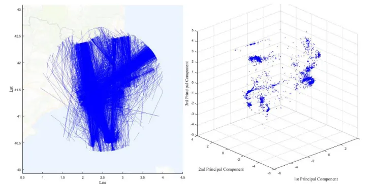
The result of these steps is presented in Figure 1. A set of trajectories is represented on the left-hand side, whereas the right-hand side illustrates the trajectories in the transformed space. The second step involves a density-based clusterisation of the n first components resulting from the first phase.

B. Density-Based Clustering Algorithms

The trajectories in the transformed space form arbitrarily shaped regions with varying densities. Gariel’s methodology proposed DBSCAN for extracting the principal clusters within the transformed space.

DBSCAN is based on the concept of dense regions. A dense region is constituted by a minimum number of points which are sufficiently close to each other. Thus, a region is defined by two parameters, the minimum number of points (min-pts) and a distance eps. DBSCAN starts visiting a point, and then checks if the neighbouring points constitute a dense region. If so, each point within the dense region is visited to search in its

surrounding for new points that may be added to the existing cluster. Once there are not new candidates to the cluster, it is closed, and the algorithm starts again with an unvisited point, until all points are labelled within a cluster or as an outlier.

Thus, DBSCAN strengths are that it does not require a prior knowledge of the number of clusters and that it is well suited to identify arbitrarily formed shapes. On the other hand, DBSCAN suffers when handling regions of different densities, because of the static nature of eps. In addition, outcomes from the algorithm are sensitive to min-pts.

Developments in density-based clustering algorithms have addressed the cluster varying density issue. The first attempt resulted in the OPTICS algorithm. OPTICS stands for Ordering Points To Identify the Cluster Structure. Main differences between DBSCAN and OPTICS reside on the nature of the solution provided by each of them. DBSCAN provides a flat partitioning of the cluster structure, whereas OPTICS enables the extraction of a hierarchical clustering [16] from a reachability plot.

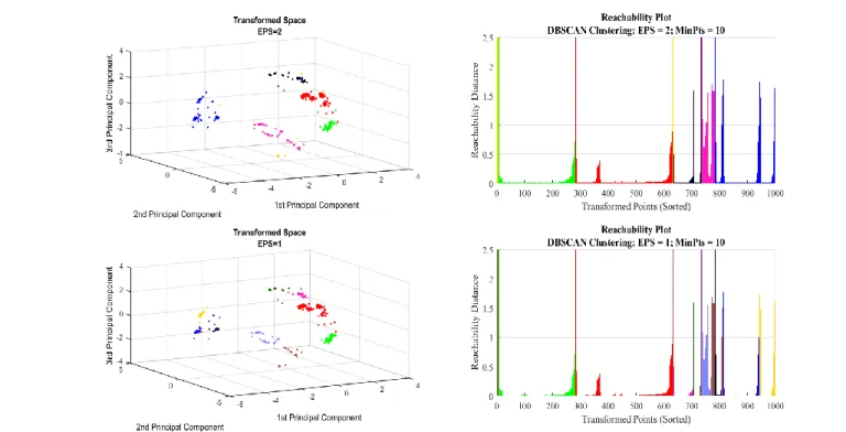
OPTICS orders the sample by reachability distances of close neighbours. The result of this ordering is a reachability plot, formed by dents and valleys. A valley between two dents would represent a dense region, as points are close among them. A dent represents a region where the distances progressively increase until a new dense region is reached. A representation of the reachability plot for a subsample from the right-hand side of Figure 1 is presented in Figure 2.

Figure 2 presents two different clustering solutions, illustrating the effect of selecting different values of eps on the original DBSCAN algorithm. The number of clusters would be

given by the number of intersections with dent left-sides. As the

eps value decreases, a higher number of clusters are detected. The last step for the OPTICS algorithm is to extract the cluster hierarchy from the reachability plot. The authors proposed the OPTICS-AutoCluster [17] algorithm, which extracts the leaf nodes of a tree built from the OPTICS reachability plot.

The last approach that will be used in this paper is HDBSCAN*, which produces a hierarchy of all possible DBSCAN* partitions, where DBSCAN* introduces a small variation from the initial version. The extraction of all possible DBSCAN* partitions is formulated as an optimisation problem over the individual qualities of the extracted clusters [8].

Both OPTICS-AC and HDBSCAN* incorporate a parameter to regulate the minimum size of the cluster. Finally, a complete description of HDBSCAN* and a complete literature review on Density-based clustering can be found in [9].

C. Density-Based Clustering Validation

Discussed density-based clustering algorithms conduct an unsupervised classification for obtaining a finite set of categories according to their similarities. Clustering results can be validated by using three different types of metrics: external; internal; and relative metrics [18].

External metrics verify clustering outcomes via known ground truth solutions, i.e. a pre-existing known solution for the cluster structure. Internal criteria refer to the assessment of the quality of the clustering solution based exclusively on the data generating it, whereas relative criteria point at comparing different clustering solutions.

Figure 2 Reachability Plot for a subsample of Figure 1. Right-hand side column represents an equal transformed space, clustered differently based on the eps value. Right-hand side colum represents the OPTICS reachability plot. Both columns are linked by colours.

External metrics, such as the Adjusted Rand Index [19], require the ground truth information about the sample. Depending on the operational environment, airspace users are mandated to follow the existing airspace route structure. Therefore, the ground truth solution for each flight would correspond to an existing sequence of segments in the route structure for the airspace volume of study. However, aircraft are often cleared out by ATC from their planned trajectories to avoid potential safety events or to expedite traffic. Air Traffic Controllers (ATCOs) often follow pre-defined patterns, based on their own experience and on the route-structure [20], [21]. Therefore, it is likely that these patterns are reflected in the clustering outcome, if track data is used for clusterisation.

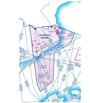
Therefore, the clusterisation of air traffic in a non-free-route airspace should uncover the route structure, but also non-conventional patterns which are derived from actual operations. An example of a conventional route-structure is illustrated in Figure 3. Therefore, clustering verification from an external point of view should combine verification against planned trajectories, and frequent patterns due to ATC actions. This leads to the need for qualitative assessment for each specific operational scenario for verification purposes in an ATC environment.

With respect to internal and relative criteria, Moulavi’s [18] strategy is replicated in this paper. Internal validity criteria metrics may be ranked, and therefore, transformed to relative validity criteria. The most common relative metric for clustering validation purposes is the Silhouette Width Criterion (SWC) [22], which compares the ratio of intra- and inter-cluster distances for evaluating compactness and separation between them. The SWC works well with globular clusters, but its performance decreases when dealing with clusters with varying forms.

The SWC is defined by means of the silhouette value. The silhouette value of a point i is defined as:

𝑠(𝑖) = 𝑏(𝑖) − 𝑎(𝑖)

max⁡(𝑎(𝑖), 𝑏(𝑖)). (1)

where a(i) is the average intra-cluster distance and b(i) is the average inter-cluster distance of the point i with points belonging to nearest cluster. Then, each cluster would be characterised by an average silhouette value (the SWC). The overall quality of the clustering solution will be given by the weighted SWC for all clusters. When the intra-cluster distance for a given point is much smaller than the inter-cluster distance, the silhouette value will tend to 1, whereas in the opposite case it will tend to -1.

Validation of clusters with arbitrary shapes and varying densities requires specific measures. Moulavi defines the Density Based Clustering Validation (DBCV) metric. This metric mirrors the notion of compactness versus separation to qualify a cluster. In this case, the compactness is defined in terms of cluster’s lower density, instead of smallest distance. The inter-cluster distance is also replaced with a inter-cluster density.

Thus, the DBCV is defined in terms of the Density Sparseness of a Cluster (DSC) and the Density Separation of a

Pair of Clusters (DSPC). Then, if we consider a set of l clusters, the validity of a cluster Ci is defined as:

𝑉𝐶(𝐶𝑖) = min 1≤𝑗≤𝑙,𝑗≠𝑖(𝐷𝑆𝑃𝐶(𝐶𝑖, 𝐶𝑗)) − 𝐷𝑆𝐶(𝐶𝑖) max⁡( min 1≤𝑗≤𝑙,𝑗≠𝑖(𝐷𝑆𝑃𝐶(𝐶𝑖, 𝐶𝑗), 𝐷𝑆𝐶(𝐶𝑖)) . (2)

If the cluster sparseness metric, i.e. lower density intra-cluster which results in higher DSC values, is larger than the cluster separation metric, then the cluster validity is negative, indicating lower relative cluster quality. More details about DSC and DSPC may be found in [18].

Finally, the Validity Index of a Clustering is defined as the weighted average of the Validity Index of all clusters in C,

𝐷𝐵𝐶𝑉 = ∑|𝐶_|𝑂|𝑖| 𝑙

𝑖=1

𝑉𝐶(𝐶𝑖), (3) where |𝑂| is the cardinality of the whole sample, including noise and |𝐶_𝑖| is the cardinality of the cluster i.

III. EXPERIMENTAL SETUP

A. Methodology

The main objective of the paper is to evaluate whether alternative density-based clustering algorithms could replace DBSCAN in the original Gariel’s methodology for automated air flow extraction or not. So far, the paper has described this methodology, most widely used density-based clustering algorithms, and relative metrics for evaluating clustering solutions without prior knowledge of the ground truth solution

Figure 3 LECBCCC Sector – Barcelona Central Sector, 2D Representation

for the sample. The methodology to carry out the evaluation is summarised as follows:

1. Given a dataset without a known ground truth, generate different clustering solutions from varying main parameters associated to the selected clustering algorithms.

2. Compute the values of the SWC and the DBCV for each solution.

3. Select the solutions associated to maximum SWC and DBCV, to qualitatively assess the obtained clusters.

Once these solutions are evaluated and discussed, the clustering algorithm that has outperformed the others will be selected.

B. Clustering Algorithms

In the previous section, three density-based clustering algorithms have been briefly introduced. These algorithms are dependent on different parameters. Thus, DBSCAN depends on

eps and min_pts for identifying the dense regions.

OPTICS-Auto Cluster (OPTICS-AC) depends on the very same min_pts parameter than DBSCAN. Additionally, OPTICS-AC depends on min_cluster_ratio, which stands for

minimum cluster ratio. This parameter defines the minimum cluster size in order to ignore regions that are too small in the reachability plot. Two additional modifications have been added for this work. OPTICS-AC outcome is a hierarchical clustering, where noisy data is not clearly identified in the pseudocode. The first modification is to only consider leaf clusters resulting from the cluster hierarchy. The second one is to apply DBSCAN to each leaf cluster with a tailored eps value, maintaining the global

min_pts. This eps parameter is defined through a KNN-search, where the min_pts-th nearest neighbour distances are selected and ordered. Then, eps is identified by means of a change point analysis [23] of this local reachability plot. Finally, HDBSCAN* inputs correspond to min_pts again, and , which is equivalent to the OPTICS-AC, but relative to min-pts.

These algorithms will be run varying their inputs, reproducing the methodology presented in [18]. Min_pts will be expressed as a ratio of the total sample size, varying from 0.5% to 5%. Eps will range between the minimum and maximum

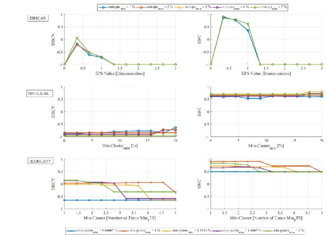
Figure 4 Quantitative metric results for different algorithms and related hyper-parameters. Rows represent different algorithms (DBSCAN, OPTICS-AC, HDBSCAN*, from top to bottom). Columns represent quantitative metrics (DBCV and SWC, from left to right).

pairwise distances that can be found in the datasets, equally distributed. In the case of , it will vary between 0.1% to 2% in the case of OPTICS-AC. For DBSCAN, it will be varying between [1, 5], relatively to min-pts.

C. Dataset

Recorded data from the sector Central (LECBCCC) within the Barcelona Air Traffic Control Centre in Spain are used in this study. The raw data correspond to one AIRAC cycle from 2014. Raw track data are reported every 4.8 seconds. A track register is composed by the timestamp, latitude and longitude in WGS84 coordinates, pressure altitude in hundreds of feet as measured by the aircraft Mode C transponder, the ground velocity vector and rate of climb or descent.

The dataset is composed by 10,313 flights. The Barcelona Central sector horizontal projection is represented in Figure 3. From North to South, and then clockwise, routes starting at PUMAL (UZ167, UN859 and UZ174) are evolution routes, entering in the cruise phase and starting the descent towards the Balearic islands. Routes UZ308 and UP84 are also descending

routes. The rest of routes are cruise routes, mainly in east-west heading.

D. Results & Discussion

The results will explore first quantitative relative indicators, and after that, a qualitative evaluation of the clustering solutions will be conducted.

About the relative indicators, results for the dataset are shown in Table I. Highest-ranked values are highlighted for each algorithm and each metric, including the values and the hyper-parameters leading to them.

Figure 4 represents the same series of data, but only plotting values for min_pts between 1% and 5% of the total sample for DBSCAN and OPTICS, and from 0.67% to 2% for HDBSCAN*.

The evaluation of DBSCAN’s results shows that both indicators have a similar behaviour with respect to the eps

parameter. It indicates that independently from the min_pts

Table I Maximum DBCV and SWC values for the different algorithms and associated hyper-parameters

Algorithm 2nd _Parameter Data Metric Min_pts 2nd Parameter Value DBSCAN - eps DBCV 1% 0.342 0.672 0.0912 SWC 0.5% 0.342 0.672 0.9054 OPTICS-AC Min_Cluster Size Ratio DBCV 1% 20% -0.634 SWC 2.5% 20% 0.7934 HDBSCAN* Min_Cluster Size Ratio / Min-pts

DBCV 2% 1 0.1471

SWC 1% 1 0.899

Figure 6 Reachability Plot for min_pts = 1% Figure 5 Clustering solutions for different min-pts ratios. The clustering algorithm is OPTICS.

variable, there is an eps value which is maximising the indicators. This value approximately coincides for both indicators, and represents approximately the location of the change of tendency on the reachability plot for the dataset, as it is illustrated in Figure 6.

The silhouette value presents a more consistent behaviour with respect to min_pts than DBCV. Remarkably, DBCV values are higher for larger values of min_pts. Figure 6 shows the transformed space for two different values of min_pts (1% and 5%) and an eps value equal to one half of the changing-trend distance for the reachability plot. Each colour represents a different clusterisation, and there is not a relation between colours of both figures.

The impact of min_pts is proved through these two figures. The left-hand side illustrates the resulting clustering for min_pts

= 1%, while its value equals to 5% for the right-hand side. If we compare both illustrations, the algorithm has achieved a more granular clusterisation for a smaller value of min_pts. Clusters on the right-hand side are larger, and more separated. This is reflected in the DBCV indicator, as it ranks higher those solutions where clusters are separated by less denser regions, i.e. there is an increased separation between clusters.

With regard to OPTICS-AC results, DBCV and SWC show a consistent performance independently from both variables. However, DBCV values are very close to -1, which would mean that the clustering solution does not achieve a good partition between clusters. This is explained from the way the hierarchical clustering is achieved in this algorithm. The algorithm seeks for maximum peaks in the ordered reachability plot for segmenting the sample. This leads to classify all the points in a cluster, without noise considerations. As it is noted in [24], DBCV is very sensitive to noise points being assigned to one cluster, which may explain low DBCV scores. In the case of the SWC,

the highest score is obtained for a very high min_cluster_size

parameter (20% of the sample). This causes that for these parameters (min_pts_ratio = 2.5% and min_cluster_size = 20%), only the most representative clusters are obtained. These clusters differentiate only aircraft by their flight phase (evolution or cruise), and main heading direction.

Finally, results for HDBSCAN* illustrate that this algorithm is more robust with respect to its hyper-parameters for both metrics. Bottom illustrations of Figure 4 show a negative tendency for both indicators as min_cluster_size increases with respect to min_pts. In any case, the highest value for DBCV for any of these algorithms is achieved by HDBSCAN*, whereas it is only slightly outperformed by DBSCAN in the case of SWC.

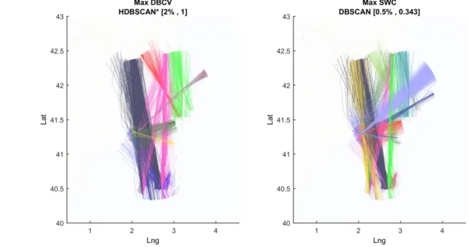
Figure 7 represents the clustering solution as a result of selecting the highest scoring solutions for both DBCV and SWC indicators. On the left-hand side, highest-ranked DBCV solution is plotted, which has been obtained through the HDBSCAN* method, whereas the right-hand side plots the trajectories for the highest-SWC solution, obtained through DBSCAN.

The qualitative assessment shows that DBCV solution has not been able to discriminate between the flows that are sharing the last part of the route denominated UZ174 in Figure 3. Best-SWC ranked solution has been able to discriminate all the main flows present in the algorithm, corresponding to a DBSCAN application.

The SWC solution was obtained after applying DBSCAN, but it does not imply that DBSCAN outperforms OPTICS-AC or HDBSCAN*, as it is very dependent on the respective parameters. DBSCAN requires two hyper-parameters, which are very dependent on the data domain. On the other hand, OPTICS and HDBSCAN* only require min_pts. In addition, both OPTICS and HDBSCAN can conduct hierarchical clustering, which is an advantage with regard to DBSCAN.

Figure 7 Track representation. The solution considering the highest ranked DBCV is plotted on the right-hand side, whereas the SWC is plotted on the right-hand side. Colours are not related between figures.

This example reflects that these indicators may fail to indicate solutions that gather all routes present in the sample only relying in the highest ranked solutions. This is due to the special nature of the data sample as a result of the PCA application to actual flight trajectories. These routes share segments, which result on clusters of points which are separated enough at microscopic level but are not at macroscopic. If hyperparameters are fine tuned to enable discrimination between those small clusters, results show that a large amount of trajectories are categorised as noise, which penalises the overall indicator values.

IV. RECURSIVE-DBSCAN I. Rationale and Pseudocode

The categorisation of an aircraft trajectory as noise or outlier is relevant for analysis purposes. DBSCAN and HDBSCAN* categorises outliers in a unique category, whereas OPTICS-AC does not describe how noise is handled. However, the identification of the outliers in the transformed space points out that outliers are also closer to some clusters than to others. The categorisation of outliers in a same general and unique category would not be reflecting that aircraft are flying a given flight route, but not in the standard manner.

Consequently, the identification of outliers in an air traffic context should be connected to actual main flows. Hierarchical clustering offers an adequate tool enabling these connections. The main idea behind RDBSCAN* is to apply recursively DBSCAN* with a varying eps parameter depending on the recursion level. For each step, eps is identified depending on the specific iteration subsample, and then, is modified depending on the recursion level.

In the first iteration, a larger eps value is desired, in order to classify only very extreme points as outliers. Then, eps shall decrement to identify only very dense areas. In each iteration, noise points are stored as a leaf node of the originating node.

The pseudocode for the algorithm is presented in Figure 8. A hierarchy is constructed based on a tree. The recursion seeks for isolating each cluster, and it stops when it only identifies the main cluster and noise. In each iteration, eps is modified accordingly, and for doing so, a decrement ratio (λ) is introduced. The recursion can also stop if the number of iterations is larger than a specified value.

Once the recursion has finished, only leaf nodes are selected as main clusters, but maintaining the noise leafs tracked with respect to their parents.

II. Experimental Setup

The experimental setup replicates the previous section one. There are different hyper-parameters for the algorithm, such

min_pts and the rate of decrement of eps. The algorithm is run for the same values that for HDBSCAN*, i.e. min_pts_ratio =

{0.1%, 2%}, whereas λ is set to 0.90. The dataset has not modified for this case.

III. Results & Discussion

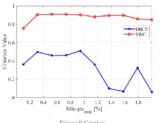
Results are presented in Figure 9 and Figure 10. The former illustrates the variation of DBCV and SWC with respect to

min_pts_ratio. It can be observed that the DBCV is significantly superior to the other algorithms. As it has been pointed out before, DBCV is very sensitive to noise, and the strength of RDBSCAN* is to hierarchically allocate outliers related to the main clusters.

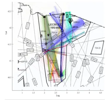
Figure 10 represents the main clusters which have been obtained for min_pts_ratio = 0.1% (equivalent to approximately

Figure 9 Caption

FUNCTION

recursiveDBSCAN(N,parent_of_N,min_pts,n_iteration) /* "Epsilon KNN: Epsilon Determination by KNN method" */

/* N is a node; the root of the tree in the first call of the procedure

// parent_of_N is the parent node of N; nil if N is the root of the tree */

eps = λ

^(n_iteration-1)*epsilonKNN(N.points,floor(min_pts))

tmp_class = dbscan(N.points,min_pts, eps);

tmp_minpts = min_pts;

/* Create a list of Ni nodes as unique classes are in

tmp_class. Each node is characterized by if it is noise and its points  NL */

IF (SIZE (L) <= 2 || n_iteration > n_iteration_limit ;

IF size(L) == 1;

// Do nothing, already inserted.

ELSEIF (SIZE(L) == 2) AND (L contains outliers)

// let N point to all nodes in NL

ELSE

FOR (Ni in NL)

n_iteration = n_iteration + 1; // let N point to Ni

recursiveDBSCAN(Ni, N,min_pts, n_iteration) END END ELSE FOR (Ni in NL) IF (Ni is an outlier) // let N point to Ni ELSE // let N point to Ni n_iteration = n_iteration + 1;

recursiveDBSCAN(Ni, N, min_pts, n_iteration)

END

END END

END FUNCTION

Figure 8 Algorithm for constructing a cluster tree recursively by using DBSCAN

min_pts = 10), where the background of the image corresponds to the sector already represented in Figure 3. After repeated iterations, it could be observed that the clustering solution that qualitatively fitted more accordingly to the route structure corresponded to a very low value of min_pts_ratio. The RDBSCAN* DBCV value outperforms DBSCAN, OPTICS-AC and HDBSCAN* due to a more tailored handling of noise considering Gariel’s methodology inner characteristics.

With respect to the qualitative analysis, it can be observed that main flows correspond to the main routes in the sector. Flows corresponding to routes UZ174 and UZ167 have been properly identified. With respect to UN13, the dataset corresponds to a sample of 2014 whereas the background is actual. It reflects that the route structure has changed to reflect actual operations by ATC. The flow coloured in yellow is also noticeable, as flights should have followed UZ308 and UZ174, but they are directed to the sector exit point from the entry point.

RDBSCAN* is a proposal for handling data where meaningful clusters are too close each other for being discriminated by means of the relative internal metrics. Additional parameters could be included to stop the recursion earlier, such as a minimum cluster size or a comparison against a well-known relative indicator such as DBCV.

V. CONCLUSIONS

Air Traffic Management systems generate huge amount of track data daily. Flight trajectories can be clustered automatically for extracting main air traffic flows by means of unsupervised machine learning techniques.

Gariel’s methodology is one of the most widely used techniques for carrying out this clusterization. This clusterization is composed by two well-differentiated steps. The first one implies a dimension-reduction of the data, whereas the second one applies a well-known density-based clusterisation algorithm (DBSCAN), to identify dense regions in this

transformed space, which later on is backtracked to the original data set of trajectories.

Advancements in density-based clusterisation algorithms have been made since the original algorithm was first presented. Two of these advancements are represented by OPTICS and HDBSCAN*.

This paper has evaluated the performance of these three algorithms by clustering air traffic data from a Spanish ATC sector. This evaluation has been conducted by means of quantitative internal metrics and qualitative evaluation of the results.

Results from the quantitative analysis have shown the difficulty to determine adequate thresholds for these indicators. This is due to factors such as the sensitivity of DBCV to noise or the special nature of the resulting dataset from the application of the first step of Gariel’s methodology.

As a main conclusion from the quantitative and qualitative analysis, it is recommended to set the min_pts hyper-parameter to the minimum value possible. This results in larger number of trajectories categorised as noise for DBSCAN and HDBSCAN*, which penalises the metrics indicators and the quality of the solution.

To overcome this issue, a recursive application of DBSCAN* is proposed, where the remaining parameter of DBSCAN* (eps) is automatically defined. In addition, the recursion creates a hierarchy, replicating this specific feature from OPTICS-AC and HDBSCAN*, which enables a more tailored categorisation of the outliers.

Quantitative evaluations show an improved behaviour on the DBCV indicator. Qualitative ones show that all main flows present in the dataset have been positively identified.

More evaluation shall be conducted about the impact of the different parameters of the first step of Gariel’s methodology on the final clusterisation. In addition, RDBSCAN* could be further developed by introducing new conditions to stop the recursion such as a minimum cluster size or a reference against an interval validity metric.

ACKNOWLEDGMENT

The author expresses his most sincere gratitude to CRIDA A.I.E. in Spain to proportionate the data and support to conduct this research.

REFERENCES

[1] F. J. Sáez Nieto, “The long journey toward a higher level of automation in ATM as safety critical, sociotechnical and multi-Agent system,” Proc. Inst. Mech. Eng. Part G J. Aerosp. Eng., vol. 0, no. 0, 2015.

[2] SESAR JU, “European ATM Master Plan 2015,” 2015.

[3] A. Eckstein, “Automated flight track taxonomy for measuring benefits from performance based navigation,” in Integrated Communications, Navigation and Surveillance Conference, 2009. ICNS’09., 2009, pp. 1– 12.

[4] M. Gariel, A. N. Srivastava, and E. Feron, “Trajectory clustering and an application to airspace monitoring,” IEEE Trans. Intell. Transp. Syst., vol. 12, no. 4, pp. 1511–1524, 2011.

[5] J. Shlens, “A Tutorial on Principal Component Analysis,” 2014. [6] M. Ester, H. H. P. Kriegel, J. J. Sander, and X. Xu, “A Density-Based

Algorithm for Discovering Clusters in Large Spatial Databases with Noise,” in Second International Conference on Knowledge Discovery and Data Mining, 1996, vol. 2, pp. 226–231.

[7] M. Ankerst, M. M. Breunig, H. Kriegel, and J. Sander, “OPTICS: Ordering Points To Identify the Clustering Structure,” 1999, pp. 49–60. [8] R. J. G. B. Campello, D. Moulavi, and J. Sander, “Density-Based

Clustering Based on Hierarchical Density Estimates,” Adv. Knowl. Discov. Data Min., pp. 160–172, 2013.

[9] R. J. G. B. Campello, D. Moulavi, A. Zimek, and J. Sander, “Hierarchical Density Estimates for Data Clustering, Visualization, and Outlier Detection,” ACM Trans. Knowl. Discov. Data, vol. 10, no. 1, pp. 1–51, 2015.

[10] M. Enriquez, “Identifying temporally persistent flows in the terminal airspace via spectral clustering,” in Tenth USA/Europe Air Traffic Management Research and Development Seminar (ATM2013), 2013. [11] E. Salaun, M. Gariel, A. E. Vela, and E. Feron, “Aircraft Proximity Maps

Based on Data-Driven Flow Modeling,” J. Guid. Control. Dyn., vol. 35, no. 2, pp. 563–577, 2012.

[12] A. Marzuoli, M. Gariel, A. Vela, and E. Feron, “Data-Based Modeling and Optimization of En Route Traffic,” J. Guid. Control Dyn., vol. 37, no. 6, pp. 1930–1945, 2014.

[13] M. Conde Rocha Murca, R. DeLaura, R. J. Hansman, R. Jordan, T. Reynolds, and H. Balakrishnan, “Trajectory Clustering and Classification for Characterization of Air Traffic Flows,” 16th AIAA Aviat. Technol. Integr. Oper. Conf., no. June, pp. 1–15, 2016.

[14] Z. Wang, M. Liang, and D. Delahaye, “Short-term 4D Trajectory Prediction Using Machine Learning Methods,” Sesar Innov. days 2017, no. November, pp. 1–9, 2017.

[15] C. E. Verdonk Gallego, V. F. Gómez Comendador, F. J. Sáez Nieto, G. Orenga Imaz, and R. M. Arnaldo Valdés, “Analysis of air traffic control operational impact on aircraft vertical profiles supported by machine learning,” Transp. Res. Part C Emerg. Technol., 2018.

[16] M. Balcan, “Robust Hierarchical Clustering ∗,” vol. 15, pp. 4011–4051, 2014.

[17] J. Sander, X. Qin, Z. Lu, N. Niu, and A. Kovarsky, “Automatic Extraction of Clusters from Hierarchical Clustering Representations,” pp. 75–87, 2003.

[18] D. Moulavi, P. A. Jaskowiak, R. J. G. B. Campello, A. Zimek, and J. Sander, “Density-Based Clustering Validation,” Proc. 2014 SIAM Int. Conf. Data Min., no. i, pp. 839–847, 2014.

[19] L. Hubert and P. Arabie, “Comparing partitions,” J. Classif., 1985. [20] J. M. Histon and R. J. Hansman, “Mitigating Complexity in Air Traffic

Control: The Role of Structure-Based Abstractions,” no. August, 2008. [21] A. Cho and J. M. Histon, “Identification of Air Traffic Control Sectors

with Common Structural Characteristics,” in 6th International Symposium on Aviation Psychology, 2011.

[22] P. J. Rousseeuw, “Silhouettes : a graphical aid to the interpretation and validation of cluster analysis,” vol. 20, pp. 53–65, 1987.

[23] W. A. Taylor, “Change-Point Analysis: A Powerful New Tool For Detecting Changes,” 2000. .

[24] T. Van Craenendonck and H. Blockeel, “Using Internal Validity Measures to Compare Clustering Algorithms,” Benelearn 2015 Poster Present., pp. 1–8, 2015