Medical Image Segmentation by Deep Convolutional Neural Networks

MEDICAL IMAGE SEGMENTATION BY DEEP

CONVOLUTIONAL NEURAL NETWORKS

Qingbo Kang

A thesis in

The Department of

Computer Science and Software Engineering

Presented in Partial Fulfillment of the Requirements

For the Degree of Master of Applied Science (Software Engineering) Concordia University

Montr´eal, Qu´ebec, Canada

August 2019 c

Concordia University

School of Graduate Studies

This is to certify that the thesis prepared

By: Qingbo Kang

Entitled: Medical Image Segmentation by Deep Convolutional Neural Net-works

and submitted in partial fulfillment of the requirements for the degree of Master of Applied Science (Software Engineering)

complies with the regulations of this University and meets the accepted standards with respect to originality and quality.

Signed by the final examining commitee:

Chair Dr. Denis Pankratov

Examiner Dr. Tien Dai Bui

Examiner Dr. Adam Krzyzak

Supervisor Dr. Thomas Fevens

Approved

Chair of Department or Graduate Program Director

2019

Dr. Amir Asif, Dean

Abstract

Medical Image Segmentation by Deep Convolutional Neural Networks

Qingbo Kang

Medical image segmentation is a fundamental and critical step for medical image analysis. Due to the complexity and diversity of medical images, the segmentation of medical images continues to be a challenging problem. Recently, deep learning techniques, especially Convolution Neural Networks (CNNs) have received extensive research and achieve great success in many vision tasks. Specifically, with the advent of Fully Convolutional Networks (FCNs), automatic medical image segmentation based on FCNs is a promising research field. This thesis focuses on two medical image segmentation tasks: lung segmentation in chest X-ray images and nuclei segmentation in histopathological images. For the lung segmentation task, we investigate several FCNs that have been successful in semantic and medical image segmentation. We evaluate the performance of these different FCNs on three publicly available chest X-ray image datasets.

For the nuclei segmentation task, since the challenges of this task are difficulty in segmenting the small, overlapping and touching nuclei, and limited ability of generalization to nuclei in different organs and tissue types, we propose a novel nuclei segmentation approach based on a two-stage learning framework and Deep Layer Aggregation (DLA). We convert the original binary segmentation task into a two-step task by adding nuclei-boundary prediction (3-classes) as an intermediate step. To solve our two-step task, we design a two-stage learning framework by stacking two U-Nets. The first stage estimates nuclei and their coarse boundaries while the second stage outputs the final fine-grained segmentation map. Furthermore, we also extend the U-Nets with DLA by iteratively merging features across different levels. We evaluate our proposed method on two public diverse nuclei datasets. The experimental results show that our proposed approach outperforms many standard segmentation architectures and recently proposed nuclei segmentation methods, and can be easily generalized across different cell types in various organs.

Acknowledgments

First of all, I would like to express my sincere gratitude to my supervisor Dr. Thomas Fevens who guides me into the deep learning and medical image processing field. Dr. Fevens is a very nice person and always inspires me to apply deep learning techniques on medical imaging problems. I really appreciate his support during the period of master study. Secondly, I want to appreciate those people who helped me with my study, research and thesis writing, including every members in our lab, thanks for their helpful discussion and corporation. Next, I would like to thank the Surgical Innovation program, the cross-disciplinary graduate program from McGill, ETS and Concordia. It provides me an unique opportunity to learn about the medical field and working with talented people from other fields: medical, business and engineering. It also provides me generous financial support and I can not finish my study in Montreal without that. Last but not the least, I want to thank my parents, for their selfless love and continuous encouragement.

Contributions of Authors

A Two-Stage Learning Framework for Nuclei Segmentation

Qicheng Lao: Color normalization, model architecture design, editing and proofing. Thomas Fevens: Research supervisor, funding, editing and proofing.

Contents

List of Figures viii

List of Tables xi

1 Introduction 1

1.1 Medical Image Segmentation . . . 1

1.2 Deep Learning for Medical Image Segmentation . . . 3

1.3 Contributions of this Thesis . . . 3

1.4 Outline of this Thesis . . . 4

2 Related Works 5 2.1 Literature Reviews for Medical Image Segmentation . . . 5

2.1.1 Lung Segmentation in Chest X-rays . . . 5

2.1.2 Nuclei Segmentation in Histopathological Images . . . 7

2.2 Convolutional Neural Network . . . 9

2.2.1 Artificial Neural Network . . . 10

2.2.2 Convolution Operation . . . 10

2.2.3 Local Connectivity and Parameter Sharing . . . 12

2.2.4 Activation Function . . . 14

2.2.5 Pooling . . . 15

2.2.6 Typical CNN Structure . . . 15

2.2.7 Training Neural Networks . . . 16

2.2.8 The Initialization of Parameters . . . 17

2.2.9 Batch Normalization . . . 18

2.3 Fully Convolutional Neural Networks . . . 19

2.3.1 FCN . . . 19

2.3.2 U-Net . . . 20

3 Lung Segmentation in Chest X-ray by Fully Convolutional Networks 24 3.1 Introduction . . . 24

3.2 Method . . . 25

3.2.2 U-Net . . . 25

3.3 Experimental Results . . . 26

3.3.1 Datasets . . . 26

3.3.2 Evaluation Metrics . . . 29

3.3.3 Implementation and Training Details . . . 30

3.3.4 Results and Discussions . . . 31

3.4 Conclusion . . . 32

4 A Two-Stage Learning Framework for Nuclei Segmentation 38 4.1 Introduction . . . 38

4.2 Motivation . . . 39

4.3 Background . . . 40

4.3.1 Stacking U-Nets . . . 40

4.3.2 Deep Layer Aggregation . . . 40

4.3.3 Curriculum Learning . . . 41 4.4 Methodology . . . 41 4.4.1 Overview . . . 41 4.4.2 Color Normalization . . . 42 4.4.3 Network Architecture . . . 42 4.4.4 Loss Function . . . 44

4.5 Experiments and Results . . . 44

4.5.1 Datasets . . . 45

4.5.2 Evaluation Metrics . . . 45

4.5.3 Implementation Details . . . 46

4.5.4 Results and Discussions . . . 48

4.5.5 Qualitative Analysis . . . 51

4.6 Conclusion . . . 52

5 Conclusion and Future Work 59 5.1 Conclusion . . . 59

5.2 Future Work . . . 60

5.2.1 More Effective Loss Function for Medical Segmentation Task . . . 60

5.2.2 More Useful Strategies for Training Deep CNNs . . . 60

5.2.3 More Deeper and Powerful Networks . . . 60

List of Figures

1 Typology of medical imaging modalities. Image is from [118]. . . 2

2 A typical fully-connected feed-forward neural network with depth 3. . . 11

3 An example of 2-D convolution operation without kernel flipping. The output in the red square is the convolution result of the red squared input region and the kernel. 11 4 Schematic diagram of local connectivity. The upper half is fully connected layer and the bottom half is locally connected layer. Image is from [48]. . . 12

5 Schematic diagram of parameter sharing. The upper half is without parameter sharing and the bottom half is with parameter sharing. Image is from [48]. . . 13

6 Some widely used activation functions in neural networks. . . 14

7 Max-pooling operation (size 2×2 and stride 2×2). . . 15

8 A typical CNN structure for a classification task. . . 16

9 The FCN-32 network structure. Green box represents pooling operation, blue box represents convolution and activation operation and red box represents up-sampling operation. . . 19

10 The skip connections in FCN. Pooling layers and prediction are shown as grids, con-volution layers are omitted for clarity. Image is from [95]. . . 21

11 The U-Net architecture. Image is from [120]. . . 22

12 The Overlap-tile strategy. Left image is input image and right image is the corre-sponding segmentation mask. Images are from [107]. . . 23

13 The architecture of FCN32 used in this study. Blue boxes represent image features. The number of features is indicated on the right of the box. The resolution of each level (features have the same resolution) is indicated on the left side of each level. . . 26

14 The architecture of FCN8 used in this study. Blue boxes represent image features. The number of features is indicated on the right of the box. The resolution of each level (features have the same resolution) is indicated on the left side of each level. . . 27

15 The architecture of U-Net used in this study. Blue boxes represent image features. The number of features is indicated on top of the box. The resolution of each level (features have the same resolution) is indicated at the bottom left of each level. . . . 28

16 Example chest X-ray images and corresponding lung segmentation masks from 3 datasets (left: MC dataset, middle: Shenzhen dataset, right: JSRT dataset). . . 29

17 Training curves (accuracy and loss) of FCN32 on 4 datasets (From up to bottom: MC, Shenzhen, JSRT, Combined). . . 33 18 Training curves (accuracy and loss) of FCN8 on 4 datasets (From up to bottom: MC,

Shenzhen, JSRT, Combined). . . 34 19 Training curves (accuracy and loss) of U-Net on 4 datasets (From up to bottom: MC,

Shenzhen, JSRT, Combined). . . 35 20 Sample segmentation results and their corresponding difference of different methods

on the MC dataset. For the difference image, white color represents True Positives (TP), black color represents True Negatives (TN), red color represents False Positives (FP) and green color represents False Negatives (FN). . . 36 21 Sample segmentation results and their corresponding difference of different methods

on the Shenzhen dataset. For the difference image, white color represents True Pos-itives (TP), black color represents True Negatives (TN), red color represents False Positives (FP) and green color represents False Negatives (FN). . . 36 22 Sample segmentation results and their corresponding difference of different methods

on the JSRT dataset. For the difference image, white color represents True Positives (TP), black color represents True Negatives (TN), red color represents False Positives (FP) and green color represents False Negatives (FN). . . 37 23 Examples of H&E stained images (up) and corresponding nuclei segmentation map

(bottom) for different organs (columns). Images are from [81]. . . 39 24 Examples of overlapping and touching nuclei, green lines outline the boundary of each

nuclei in H&E stained images. Images are from [81]. . . 39 25 The shallow aggregation, IDA and HDA. Image is from [156]. . . 41 26 Example image samples (up) and their corresponding color-normalized image samples

(bottom). The first column is the target image. Images are from [81]. . . 42 27 The architecture of our proposed segmentation network. Blue boxes represent image

features. The number of features is indicated on top of the box. The resolution of each level (features have the same resolution) is indicated at the bottom left of each level. . . 43 28 Example images (up) and associated ground truth segmentation masks (bottom) of

the TNBC dataset. . . 46 29 Example images (up) and associated ground truth binary masks (middle) and

associ-ated ground truth nuclei-boundary masks (bottom). The first two columns are from the TCGA dataset while the last one from the TNBC dataset. . . 47 30 Comparative analysis of AJI for each organs on the TCGA test set. . . 49 31 Comparative analysis ofF1 scores for each organs on the TCGA test set. . . 50

32 Overall segmentation results. Example input H&E stained images (first column) and associated ground truth (second column) and corresponding binary output (third column) and nuclei-boundary output (forth column). Here we use the outputs of our best model (Ours (DLA)). The images of first three rows are from the TCGA dataset and the last one come from the TNBC dataset. . . 53 33 Segmentation results of different methods for different organs (liver, kidney, bladder

and breast) on the TCGA dataset. White area indicates True Positives, black area indicates True Negatives, while red area represents False Positive and green area represents False Negative. The associated AJI andF1score are shown on the bottom

of each result image. . . 54 34 Segmentation results of different methods for different organs (prostate, colon and

stomach) on the TCGA dataset. White area indicates True Positives, black area indicates True Negatives, while red area represents False Positive and green area represents False Negative. The associated AJI andF1score are shown on the bottom

of each result image. . . 55 35 Segmentation results of different methods for different patients on the TNBC dataset.

White area indicates True Positives, black area indicates True Negatives, while red area represents False Positive and green area represents False Negative. The associ-ated AJI andF1 score are shown on the bottom of each result image. . . 56

36 Segmentation results of small nuclei. Example input H&E stained images (first col-umn) and associated ground truth (second colcol-umn) and corresponding segmentation result of U-Net (third column) and corresponding segmentation result of our model (the last column). . . 57 37 Segmentation results of overlapping and touching nuclei. Example input H&E stained

images (first column) and associated ground truth (second column) and corresponding segmentation result of U-Net (third column) and corresponding segmentation result of our model (the last column). . . 58

List of Tables

1 Details of the chest X-ray image datasets used in this study. . . 30 2 Lung segmentation results of different methods. . . 31 3 Composition of the TCGA dataset and the associated training/testing protocol. . . . 45 4 Results by choosing different loss weightα. . . 48 5 AJI of different methods on the TCGA test set. . . 48 6 F1 scores of different methods on the TCGA test set. . . 49

7 AJI and F1 scores of different methods on the same organ testing set and different

organ testing set of the TCGA dataset. . . 50 8 Quantitative comparison of different methods on the TNBC dataset. . . 51

Chapter 1

Introduction

In the first chapter, I will give a brief introduction of my thesis. First of all, I will describe the medical image segmentation problem. Secondly, how the deep learning techniques used for medical image segmentation will be discussed. Thirdly, the contributions of this thesis will be mentioned and finally, I give the outline of this thesis.

1.1

Medical Image Segmentation

Medical imaging techniques play a prominent role and have been widely used for the detection, diagnosis, and treatment of diseases [14]. There are many medical imaging modalities including X-ray, computed tomography (CT), magnetic resonance imaging (MRI), ultrasound, positron emission tomography (PET) and so on. A typology of common medical imaging modalities used for different parts of human body which are generated in radiology is shown in Fig. 1.

Since this thesis focus on X-ray images and pathological images, we provide some details about these two kinds of imaging techniques in the following.

X-ray Images Since the German physicist Roentgen discovered X-rays in 1895, X-ray images have been used for clinical diagnosis for more than 100 years. Medical X-ray images are electron density metric images of different tissues and organs in human body. X-ray based imaging including 2D computer radiography, digital X-ray photography, digital subtraction angiography, mammography and 3D spiral computed tomography, etc., have been widely used in orthopedics [129], lungs , breast and cardiovascular [106] and other clinical disease detection and diagnosis. However, 2D X-ray images can not provide three-dimensional information of human tissues and organs. The automatic identification for 2D X-ray images is also difficult since there are overlaps in tissues and organs. Pathological Images Pathological images refer to cutting a certain size of diseased tissue, using hematoxylin and eosin (H&E) or other staining methods to make the sliced tissue into a pathological slide, and then utilizing microscopic imaging techniques for cells and glands. By analyzing the pathological images, the causes, pathogenesis of the lesions can be explored to make a pathological

Medical Image Modalities Histology Computed Tomography (CT) Magnetic Resonance Imaging (MRI) Positron Emission Tomography (PET) Ultrasound X-rays Epithelium Endothelium Cells Nuclei Placenta Abdomen Bladder Brain Chest Kidney Cervix Neuroimaging Cardiovascular Liver Oncology Cardiology infected tissues Neuroimaging Oncology Musculoskeletal Pharmacokinetics Transrectal Breast Abdominal Transabdominal Cranial Gallbladder Spleen Mammography Fluoroscopy Arthrography Discography Dexa Scan Chest

Figure 1: Typology of medical imaging modalities. Image is from [118].

diagnosis. Recently, with the advent of whole-slide imaging (WSI), it can obtain tumor spatial information such as nuclear direction, texture, shape, and structure and allows quantitative analysis of sliced tissue. A prerequisite for identifying these quantitative features is the need of detection and segmentation of histological primitives such as nuclei and glands [99].

Medical image segmentation is a complex and critical step in medical image processing and anal-ysis. The purpose of medical image segmentation is dividing an image into multiple non-overlapping regions based on some criterion or rules such as similar gray level, color, texture etc.. Based on var-ious traditional techniques, many researchers proposed a great number of automated segmentation approaches such as thresholding, edge detection, active contours and so on [115, 123]. After that, machine learning based methods have dominate this field for a long period. Machine learning rely on hand-crafted features, therefore how to design suitable features in different field and different

imaging modalities has become a primary concern and a key factor for the success of such a segmen-tation system. However, due to the complexity and diversity of medical images, the segmensegmen-tation of medical images continues to be a challenging problem.

1.2

Deep Learning for Medical Image Segmentation

Deep learning has been widely used and achieves great success in many areas such as computer vision, speech analysis and natural language processing [83]. In contrast to traditional machine learning techniques which based on hand-craft features for different task, deep learning directly learns representation features from huge amount of data. Specific to medical image segmentation field, deep leaning techniques based approaches especially approaches based on Convolution Neural Networks (CNNs) have received extensive attention and research, many works have been proposed and achieved superior performance compared to segmentation methods based on other techniques [94, 124]. Many CNNs based segmentation network such as FCN [95], U-Net [120], V-Net [102] and their variants or improvements [28, 39, 162, 76, 110, 3, 114, 51, 50] have been proposed and achieve state-of-the-art performance on numerous medical image segmentation tasks.

1.3

Contributions of this Thesis

In this thesis, we focus on two medical image segmentation tasks, lung segmentation in chest X-ray images and nuclei segmentation in histopathological images.

For the lung segmentation problem, we apply FCN and U-Net, the two most widely used seg-mentation model for medical image segseg-mentation, on this task. We evaluate the performance of these models on three publicly available chest X-ray datasets, the experimental results demonstrate the superior performance of deep learning based segmentation models.

For the nuclei segmentation problem, we propose a novel nuclei segmentation approach based on a two-stage learning framework and Deep Layer Aggregation (DLA) [156]. We convert the original binary segmentation task into a two-step task by adding nuclei-boundary prediction (3-classes) as an intermediate step. To solve our two-step task, we design a two-stage learning framework by stacking two U-Nets. The first stage estimates nuclei and their coarse boundaries while the second stage outputs the final fine-grained segmentation map. Furthermore, we also extend the U-Nets with DLA by iteratively merging features across different levels. We evaluate our proposed method on two public diverse nuclei datasets. The experimental results show that our proposed approach outperforms many standard segmentation architectures and recently proposed nuclei segmentation methods, and can be easily generalized across different cell types in various organs.

1.4

Outline of this Thesis

This thesis is organized as follows: Chapter 2 will reviews some related works of this thesis, specif-ically the literature reviews for the two segmentation tasks, some details of CNN and two segmen-tation model: FCN and U-Net. Chapter 3 will presents our lung segmensegmen-tation work in chest X-ray images and the associated experimental results. Chapter 4 will presents our nuclei segmentation work and the corresponding experimental results. In Chapter 5, we will conclude this thesis and discuss some future work and research directions.

Chapter 2

Related Works

This chapter will cover related works of this thesis. Specifically I will briefly review some literature for the two segmentation tasks which this thesis focuses on, i.e. lung segmentation in chest X-rays and nuclei segmentation in histopathological images. After literature reviews, CNNs and the Fully Convolutional Neural Networks will be described in this chapter.

2.1

Literature Reviews for Medical Image Segmentation

2.1.1

Lung Segmentation in Chest X-rays

Over the past decades, researchers have proposed a number of methods to segment the lung field from chest X-ray images. These methods can be divided into four categories [141, 62]: rule-based segmentation [116, 149, 15, 18, 89], pixel classification-based segmentation [101, 55, 145, 138, 5, 142, 25], deformable model-based segmentation [67, 157, 4, 32, 140, 125, 52] and hybrid segmentation [142, 34, 17].

Rule-based Segmentation

The rule-based segmentation methods aim to obtain the expected target region of interest after image pixels are processed through a series of steps and rules. Most of the early proposed lung field segmentation algorithms fall into this category [116, 149, 15]. Some techniques like threshold segmentation, region growth, edge detection, ridge detection, mathematical morphology, geometric models, and so on are used to find the edge of the lung area based on the characteristics of lung structure [18, 89].

Pixel Classification-based Segmentation

A series of feature vectors are calculated for each pixel in the image, and some pattern recognition techniques are used to mark the category of each pixel belongs to according to the feature vector [101]. For the digital X-ray chest radiology segmentation problem, the pixel classification method is to assign each pixel in the chest radiograph image with the corresponding anatomical structure (such as lung and background, or heart, mediastinum and diaphragm, etc.) through a classifier. The classifier can use pixel point gray information, spatial position information, texture statistics information, etc. as feature vectors then obtain the labels through training of neural network [55, 138, 5], K nearest neighbor (KNN) classifier [142], support vector machine (SVM) [25], Markov random field model [145], etc.

Deformable Model-based Segmentation

The segmentation method based on deformable model belongs to the top-down strategy. Firstly, an overall model for understanding the target is generated according to the content of the image, and then the image feature is applied to fit the model to the best match and the target object is segmented. After more than 20 years of research, from elastic model, active contour model [67, 157, 4] to active shape model [32, 140, 125, 52], the deformable model has been developed and widely used in the field of image segmentation. In the field of lung segmentation, active contour models and active shape models have received the most attention from researchers. Iglesias et al. [67] first use the active contour model with shape constraints for lung segmentation, and studied the effects on the segmentation results of different parameters in the active contour model. Yuet al. [157] propose a lung segmentation method based on shape regularized active contour. Annangiet al. [4] present a work by using level set energy to segment the lungs from chest X-rays. Cooteset al. [32] propose active shape models. Vanet al. [140] present a segmentation method based on active shape models with optimal features. Shiet al. [125] use the active shape model based on scale-invariant feature transform (SIFT) features to segment the lungs. Guo and Fei [52] develop a minimal path searching method for active shape model based segmentation for chest X-rays.

Hybrid Segmentation

Combining multiple segmentation methods and overcoming shortcomings of one method by another method. It is hoped that the combined use of multiple methods can complement each other and make the segmentation result better. After using the Active Shape Model (ASM), Active Appear-ance Model (AAM), and Pixel Classification (PC) to segment the lungs, Van Ginneken et al.[142] proposed a joint ASM, AMM, and PC method to segment images. In order to obtain the inde-pendent segmentation results of the pixels of ASM, AMM, and PC, each pixel is voted by using the classification results of the three methods, and each pixel is classified according to the majority principle. Another strategy is utilizing the segmentation result of one method as the input of another method for the second segmentation, such as ASM/PC, PC/ASM, and so on. Candemiret al. [17] present a hybrid method based on nonrigid registration and anatomical atlas as a guide combined

with graph cuts for refinement.

2.1.2

Nuclei Segmentation in Histopathological Images

Nuclei segmentation has been studied for decades and a large number of methods have been proposed [147]. Most of the traditional nuclei segmentation methods based on these following algorithms: in-tensity thresholding (such as OTSU [112, 150, 122]), image morphological operations [160], watershed transform algorithm [151, 144], active contours [73, 111, 104, 29, 19, 100, 153, 20, 148, 21, 143, 54, 35, 137], clustering (such as K-means [98] ), graph-based segmentation methods [42], supervised classification and their variants or combinations.

Intensity Thresholding

The most basic and simplest algorithm for nuclei segmentation may be intensity thresholding. Using a global threshold value or some locally adaptive threshold values to convert the input image to a binary image is widely used in image processing field. The method for choosing the specific thresholding value is related to the task and the input image. Specific for nuclei segmentation, the intensity distribution of pixel values between nuclei (foreground) and the background is persistently distinct. One of the most famous locally adaptive algorithms is OTSU [112], which selects a threshold by maximizing the variance between the foreground and the background. In order to tackle the problem of non-consistent intensity values within an image, an extension of this method is to divide the full image into numerous sub-images and perform thresholding individually [122], but it requires additional parameters thus can’t perform automatically.

Image Morphological Operations

Mathematical morphology is one of the most widely used techniques in image processing field. The basic operations including erosion, dilation, opening and closing. For nuclei segmentation task, morphological operations often cooperate with other methods to achieve better segmentation performance. For example, [160] presents an unsupervised nuclei segmentation method which using morphology to enhance the gray level values of the nuclei.

Watershed

Watershed transform is one of the most important image segmentation algorithms. It can be clas-sified as a region-based segmentation method which utilizing a region growing strategy, specifically, it starts with some seed points and then iteratively adds image pixels which satisfies some require-ments to regions. [151] proposed a marker-controlled watershed to avoid over-segmentation problem in segmenting clustered nuclei. [144] utilized marker-controlled watershed segmentation for nuclei segmentation in H&E stained breast biopsy images.

Active Contours

Active contour models or deformable models are extensively studied and used for nuclei segmenta-tion. With some initial starting points, an active contour evolves toward the boundaries of desired region or objects by minimizing an energy functional. The energy of the active contour model (also known as Snake) is formulated as a linear combination of three terms [73]: internal energy, image energy and constraint energy. The internal energy controls the smoothness and continuity of the con-tour, the image energy encourages the Snake to move toward features of interest and the constraint energy can be based on the specific object. The two major implementations of active contour models for nuclei segmentation are geodesic snakes (or level set models) which are with implicit contour rep-resentations and parametric snakes which are with explicit contour reprep-resentations [147]. A contour is implicitly represented as the zero level set of a high-dimensional manifold in a geodesic model [35, 111]. There are mainly two types geodesic models: edge-based level set models [19, 100, 153, 20] which rely on the image gradient to terminate contour evolution and region-based level set models [21, 143] which based on the Mumford-Shah functional [104]. Region-based models are more robust to noise and weak edges compared with edge-based models [147]. Hanet al. [54] present a topology preserving level set model to preserve the topology of the implicit curves or surfaces throughout the deformation process. Taheriaet al. [137] propose a nuclei segmentation approach which utilizes a statistical level set approach along with topology preserving criteria to evolve the nuclei border curves. While in a parametric active contour model, a continuous parameter is explicitly used to represent a contour. The traditional Snake model [73] moves contours toward desired image edges while preserving them smooth by searching for a balance between the internal and external force. A balloon snake [29] is formed by introducing a pressure force to increase the capture range of the ex-ternal force. On the other hand, [148] replaced the exex-ternal force with a gradient vector flow (GVF) to handle the problems of poor convergence to boundary concavities and sensitive initialization. Clustering

Clustering is the process of dividing a collection of data objects into multiple subsets. Each subset is called a cluster. Clustering makes the objects in the cluster have high similarity, but it is not very similar to objects in other clusters. Different clustering algorithms may produce different clusters on the same dataset. Cluster analysis is used to gain insight into the distribution of data, observe the characteristics of each cluster, and further analyze the characteristics of specific clusters. Since a cluster is a subset of data objects, the objects in the cluster are similar to each other and not similar to the objects in other clusters. Therefore, the cluster can be regarded as a ”recessive” classification of the dataset, and cluster analysis may find the unknown subset of the dataset. Clustering is unsupervised learning, unsupervised learning refers to the search for implicit structural information in unlabeled data. For nuclei segmentation task, clustering is usually used as an intermediate step such as extract object boundary. Popular clustering algorithms including K-means [98], Fuzzy c-means [10] and EM algorithm [36]. [78] presented a K-c-means clustering based approach for nuclei segmentation in H&E and immunohistochemistry (IHC) stained pathology images. [6] designed a nuclei segmentation method based on manifold learning which utilizing K-means to segment nuclei

and nuclei clumps. [16] proposed a parallel Fuzzy c-means based approach for nuclei segmentation in large-scale images, which can be used to process image which has high resolution such as WSI. Graph-based Methods

A graph-based image segmentation method [42] treats an image as a weighted graph. Each node in the graph represents a pixel or super-pixel in the image, and each edge weight between the nodes corresponds to the similarity of adjacent pixels or super-pixels. In this way, a graphic can be divided into multiple regions according to a criterion, each region represents an object in the image. Typical example graph-based methods including Max-Flow/Min-Cut algorithms [49, 13, 12], normalized cut [146] and Conditional Random Fields (CRF) [82]. The Max-Flow/Min-Cut algorithms solve the image segmentation problem by minimizing an energy function. While the normalized-cut algorithm attempts to divide the set of vertices of an undirected graph into multiple disjoint classes, so that the similarity between classes is very low, the similarity within the class is very high, and the size of the class should be as balanced as possible. CRF formulates segmentation task as a pixel-wise classification or labelling task and assigns the labels of each pixel or super-pixel based on the observations, this method can be classified as a discriminative graphical model.

Supervised Classification

A number of nuclei segmentation methods based on supervised machine learning have also been proposed. There are two categories methods for this task, i.e. pixel-wise classification or superpixel-wise classification. For pixel-superpixel-wise, the label of each pixel of determined by a learned model with some criteria. While for superpixel-wise classification, a set of candidate regions for nuclei are first segmented from the input by a learned model. The general pipeline of this method is first apply some feature extraction algorithms to extract image features from input image and then feed into classifiers such as K-NN, SVM [133], Bayesian, etc. [77] presents a supervised learning algorithm for nuclei segmentation in follicular lymphoma pathological images. The local Fourier transform features are firstly extracted from the image, then a K-NN classifier is applied to determine the label of each pixel.

2.2

Convolutional Neural Network

Deep learning [48] has been widely used and achieved notable success in many domains such as computer vision [79, 128, 119, 95, 45], natural language processing [30, 31, 154], speech recognition [60, 37, 161]. CNNs [86] are a special kind of feed-forward network with sparse connectivity and parameter sharing, which are particular designed for dealing with data that has grid-like topology such as image data [48]. CNNs have achieved remarkable performance in plenty of computer vision tasks including image classification [79, 128, 58, 59, 63], image segmentation [95, 109, 7, 56, 24], face recognition [113, 22], image style transfer [45, 96] etc.

CNNs are motivated by the mechanism of receptive field in biology. In 1959, David Hubel and Torsten Wiesel discovered that there are two types of cells in cat’s primary visual cortex: simple

cells and complex cells. These two kinds of cells responsible for tasks in different levels of visual perception [64, 65, 66]. The receptive field of the simple cell is long and narrow, and each simple cell is only sensitive to the light with the specific orientation in the field, while the complex cell is aware of the light of an orientation in the field moving along a specific direction. Inspired by this observation, in 1980, Kunihiko Fukushima proposed a multi-layer neural network with convolution and sub-sampling operations: Neocognitron [44]. After that, Yann LeCun introduced the back-propagation (BP) algorithm into CNNs in 1989 [84] and achieved great success in handwritten digit recognition [85].

AlexNet [79] is the first modern deep CNN model, which can be considered as the beginning of a real breakthrough of deep learning techniques for image classification. AlexNet does not require pre-training and layer-wise training, on the contrary, it uses many techniques that are widely used in modern deep CNNs, such as parallel training using GPU, ReLU as a nonlinear activation function, dropout [61, 130] to prevent over-fitting, and data augmentation to improve the performance of the model, etc. These techniques have greatly promote the development of end-to-end deep learning models. There are many CNN models have been proposed after AlexNet, such as VGG [128], Inception v1 [135], v2 [136], v4 [134], ResNet [58, 59] DenseNet [63] and so on.

Currently, CNNs have become the dominating models in the field of computer vision. By intro-ducing skip connection across layers, the depth of a CNN may beyond one thousand layers. However, no matter how deep a CNN model is, the basic building blocks of it stay the same. In general, it may consists of convolution layers, pooling layers and fully-connected layers. This section will give some details of each building blocks in a CNN model.

2.2.1

Artificial Neural Network

Artificial Neural Networks (ANNs) are artificial computational systems which were mainly motivated by biological neural systems in human brain. The most fundamental element in ANNs is neurons or nodes, a typical ANN consists of numerous neurons and weighted connections between these neurons. Neurons receive input signals from connections and perform some operations then generate outputs [70, 152]. Neurons are grouped by layer and ANNs may have multiple layers, the number of layers is called the depth of ANNs. An ANN can be trained to approximate a particular function by adjusting the weights of connection. According to the connection pattern, ANNs can be divided into feed-forward networks in which there is no loop or feedback connections, and recurrent networks in which there has feedback connections [48]. In particular, a feed-forward network with all neurons in current layer have connections with all neurons in the next layer is called fully-connected network. Fig. 2 shows an example of 3 layers (input layer, hidden layer and output layer) fully-connected feed-forward network.

2.2.2

Convolution Operation

Convolution operation initially is an important operation in mathematics, it also has a broad usage in signal and image processing. Since the convolution used in neural networks has some slightly differences compared to the convolution used in pure mathematics, the convolution described here is

input layer

hidden layer

output layer Weight Matrix

Weight Matrix

Figure 2: A typical fully-connected feed-forward neural network with depth 3.

just used in neural networks. When apply on imaged, the convolution usually has a two-dimensional discrete form. Formally, letI be an image and K be a kernel, the two-dimensional discrete convo-lution is: P(i, j) = (I∗K)(i, j) = i X u=0 j X v=0 I(u, v)K(i−u, j−v) (1)

where the range ofuis [0, i) and the range ofvis [0, j),iandjare the width and height of the kernel, respectively. In the context of deep learning and image processing, the main function of convolution is to obtain a new set of features or representations by sliding a convolution kernel (i.e. filter) on an image. In practice, many deep learning libraries such as TensorFlow [1], Theano [9] and Caffe [72] use cross-correlation operation instead of convolution operation, which can reduce unnecessary computation cost significantly. Given an imageI and kernelK, the cross-correlation is defined as:

P(i, j) = (I∗K)(i, j) = i X u=0 j X v=0 I(i+u, j+v)K(u, v) (2)

For the purpose of feature extraction, convolution and cross-correlation are equivalent, the only difference between convolution and cross-correlation is whether the kernel is flipped. Fig. 3 shows an example of 2-D convolution operation without kernel flipping.

input

kernel

output

*

=

1

-1

-2

-1

0

-1

1

0

0

1

1

2

1

0

0

-1

0

-2

0

0

2

2

Figure 3: An example of 2-D convolution operation without kernel flipping. The output in the red square is the convolution result of the red squared input region and the kernel.

2.2.3

Local Connectivity and Parameter Sharing

Compared to ordinary neural network layers, convolution layer has two important properties: local connectivity and parameter sharing.

Local Connectivity

1

2

3

4

5

1

2

3

4

5

1

2

3

4

5

1

2

3

4

5

Figure 4: Schematic diagram of local connectivity. The upper half is fully connected layer and the bottom half is locally connected layer. Image is from [48].

All the neurons in one convolution layer only connect with neurons in a small local region of previous layer. The local region is called the receptive filed of this neuron. Local connectivity (also known as sparse connectivity, sparse weights and sparse interactions) ensures that the learned filter has the strongest response to local input features and also can decrease the number of parameters of a CNN model dramatically. Fig. 4 schematically illustrates the local connectivity property. More precise, the upper half of Fig. 4 shows the connectivity pattern of a fully connected layer while the bottom half describes the local connectivity pattern of a convolution layer. In the upper half, the above row is the matrix multiplication result with fully connectivity, the blue circles in the bottom

row affect the result output y3 and are called the receptive field of y3. Since it’s fully connected,

all the inputs affecty3. While in the bottom half, the above row is the convolution result of kernel

with width 3 applies on the bottom row. With local connectivity, only 3 inputs affecty3.

Parameter Sharing

1

2

3

4

5

1

2

3

4

5

1

2

3

4

5

1

2

3

4

5

Figure 5: Schematic diagram of parameter sharing. The upper half is without parameter sharing and the bottom half is with parameter sharing. Image is from [48].

In a CNN, the parameters are the same for a convolution operation applies for every neurons in one layer. This means for one layer, we do not need learning separate sets of weights for every location, we just need learning one set of weights and then applying them everywhere. This property further reduces the number of parameters. Fig. 5 demonstrates the parameter sharing property. The red arrows in Fig. 5 represent the connections that use an unique parameter in two different situations. In the upper half, the situation without parameter sharing, the parameter is unique and used only once. While in the bottom half, the parameter of the central element of a convolution of kernel with width 3 is used at all input locations because of parameter sharing.

2.2.4

Activation Function

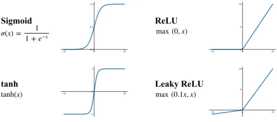
The main purpose of an activation function in a neural network is to provide nonlinear modeling ability for the neural network. A neural network without nonlinear activation function can only express linear mapping, and no matter how many layers this network has, it is equivalent to one single-layer neural network. In general, neurons receive some input signals, perform some operations or functions such as weighted sum, and optionally followed by nonlinear activation functions. Typical activation functions including Sigmoid, tanh, Rectified Linear Units (ReLU) [105] and Leaky-ReLU [97]. Fig. 6 gives the corresponding formula and figure of some widely used activation functions in neural networks.

tanh

ReLU

Sigmoid

Leaky ReLU

Figure 6: Some widely used activation functions in neural networks.

The Sigmoid function is the most widely used non-linear activation function historically, it con-verts the continuous real-valued input to an output between 0 and 1 and particularly suitable for classification problems. But in recent years, it has fallen out of favor and rarely ever used since it has three major drawbacks. The first drawback is that it can saturate and kill gradients and cause gradient exploding/vanishing problem [47]. The second drawback of Sigmoid is the outputs is not zero-centered and this will slow down the convergence of deep neural networks. The last drawback is that the Sigmoid has a power operation which is a relatively time-consuming operation and will increase the training time for deep networks. The tanh function solves the second drawback of Sigmoid, i.e. the not zero-centered problem, but the gradient exploding/vanishing and the power operation problems still exist. The ReLU solves the gradient exploding/vanishing problem in posi-tive interval and is computational efficient but the outputs of ReLU is not zero-centered. It also has dead ReLU problem which means some neurons may never be activated (the corresponding param-eters never be updated). However, the ReLU function is still the most commonly used activation function nowadays [79]. In order to tackle the dead ReLU problem, the Leaky ReLU function was proposed [57] which has a small negative slope. In theory, the Leaky ReLU is better than ReLU since there will be no dead ReLU problem, but in practice, it does not fully prove that the Leaky ReLU is always better than ReLU.

There are a great number of activation functions used in neural networks and each of them has different properties, how to choose the right activation function is depending on the specific task you are perform (i.e. the function that you are trying to approximate). In addition, different activation functions can be used in different layers in one CNN architecture, for example, many deep CNNs for image classification use ReLU as activation function in hidden layers and use Sigmoid as activation function in output layer [79, 128, 135].

2.2.5

Pooling

Pooling layer, also known as sub-sampling layer, it performs down sampling operation on the feature maps thus decreasing the dimension of feature maps and thereby reducing the number of parameters. Since pooling operation summaries some statistics of the neighboring outputs in previous layer, it enables the feature representations after pooling operation approximately unchanging to small translation. The size of the pooling layer is the window size which used for calculation, and the stride of the pooling layer is the number of pixels between every calculation. There are two commonly used pooling functions: max-pooling which choose the maximum value and average-pooling, in contrast, selects the average value. Fig. 7 illustrates a max-pooling operation with size 2×2 and stride 2×2.

0 4 2 0 0 1 2 2 0 0 3 0 3 4 1 3 1 3 1 0 Input Feature Maps

Output Feature Maps

Input Feature

Output Feature Max-pooling

Figure 7: Max-pooling operation (size 2×2 and stride 2×2).

2.2.6

Typical CNN Structure

For a classification task, the architecture of a typical CNN is composed of a stack of convolution layers, pooling layers and fully-connected layers. At present, the pattern of most widely used CNN structure is shown in Fig. 8. A convolution layer usually involves a convolution operation followed by an activation function. A convolution block consists of successive M convolution layers and b

pooling layers. N consecutive convolution blocks can be stacked in a CNN, finally followed byK

fully-connected layers.

Convolution Activation Pooling

× M × b × N Fully-connected × K softmax input

Figure 8: A typical CNN structure for a classification task.

The purpose of fully-connected layers in a classification task is to map the result features of the convolution layers and pooling layers to class labels. Clearly, since the fully-connected layers have a huge number of parameters, they are wasteful and cost a large amount of computational power, thus cannot scale to large input image. In some CNN architectures such as GoogLeNet [135], there is no fully-connected layers.

2.2.7

Training Neural Networks

Training of a neural network means solving one particular case of optimization problem: finding the parameters or the weights of the connectionsθ in a neural network that minimize a predefined loss functionL(Y, f(X, θ)). The loss function measures the performance of the neural network on the data , specifically, it evaluates the degree of inconsistency between the predicted labelsf(X, θ)of the model given the current weightsθof the model and the ground truth labelsY. Two commonly used loss functions are Mean Squared Error (MSE) and Cross-Entropy (CE). MSE calculates the average of the squared differences between the predicted labels and the true labels:

MSE = 1 m m X i=1 (Yi−Yˆi)2 (3)

where m is the number of data samples and ˆYi is the i-th predicted label. MSE is usually used

in regression problem, while CE is often used in classification problem, for a binary classification problem (i.e. Yi ={0,1}), the CE can be defined as:

CE =−1 m m X i=1 (Yilog ˆYi+ (1−Yi) log(1−Yˆi)) (4)

where Yi and ˆYi are the ground truth labels and predicted labels, respectively. In the context

of machine learning, gradient based learning algorithms are widely used to train neural networks. Specifically, BP algorithm [84] is used to compute the gradients for each parameter based on the total loss value of the model. The core idea of BP is utilizing chain rule repeatedly to calculate partial derivatives for each parameter in the model. Basically, it starts from the last layer, calculates

the error vector in reverse, continuously applies the chain rule to calculate the loss value of the cumulative gradient inversely, thus minimizes the loss function. After obtain all the gradients, gradient based learning algorithms is generally used to update the parameters. Specifically, gradient descent technique add an appropriate negative gradient on the original parameter:

θn+1=θn+ ∆θ(n)

∆θ(n) =−α ∂L ∂θ(n)

where αis called learning rate,L is the total loss value andnis the iteration number. When just part of the examples (mini-batch) from the training set are used for loss function calculation, the algorithm used for updating parameters based on this loss value is known as stochastic gradient descent (SGD). Since different initialization strategies of the parameters and the use of only partial samples during the parameter update process, SGD can only find the local optimal solution.

Based on the gradient descent learning algorithm, many optimization algorithms for training neural network are proposed. Momentum [117] is a method designed for accelerating learning process of SGD by introducing a hyper-parameter called momentum which is derives from physical analogy. Recently, many adaptive learning rate based optimization methods have been introduced, such as AdaGrad [40], Adam [75] and AdaDelta [158].

The training process can be divided into two categories, online learning and batch learning. Online learning usually selects one data sample randomly from the training set then learn one by one. The main advantage of online learning is small computational cost, however it converges pretty slow. Batch learning utilizes all data samples in the training set which benefits the loss calculation based on all data, but the computation is huge and only suits for the situation when has very small data samples. In practice, the most widely used training strategy is mini-batch learning which is a trade-off between the above mentioned two categories. Generally, the traversing of the entire training set of learning process is defined as one epoch.

2.2.8

The Initialization of Parameters

The initialization strategy of parameters in a CNN model has a big influence on the convergence speed and the performance of the model. Next, three most widely used parameters initialization methods will be described.

Gaussian Initialization

In this initialization, parameters are initialized with random values which selected from a specified Gaussian distribution N(µ, σ2_{), the mean value and the variance of the Gaussian distribution are}

pre-defined and fixed. Xavier Initialization

Xavier initialization was proposed by Glorot and Bengio [47], the initial variance of Gaussian distri-bution is no longer pre-defined and fixed but determined by the input layer of the current layer and

the number of neurons in the input layer. Suppose the number of neurons in the input layer isnin,

and the number of neurons in the output layer isnout. The initial variance is:

V ar= 2

nin+nout

(5) then a Gaussian distribution with zero mean andV arvariance is used for parameters initialization. MSRA Initialization

MSRA initialization was presented by He et al. [57]. Unlike the Xavier initialization, MSRA ini-tialization uses different initial variance for Gaussian distribution to obtain a much more robust initialization. The initial variance of MSRA is:

V ar= r 2 nl nl=k2ldl−1 (6)

whereklis the kernel size of convolution, anddl−1 is the number of convolution kernel in (l−1)-th

layer.

In conclusion, Xavier initialization is more suitable for the network which uses Sigmoid as acti-vation while MSRA initialization works better for the network uses ReLU as actiacti-vation.

2.2.9

Batch Normalization

Training deep neural networks including deep CNNs is extremely challenging, one of the most impor-tant reasons is that deep neural networks may consist of a large number of layers, and the parameters of all layers are updated simultaneously. Every parameter update in one layer will change the input data distribution of all subsequent layers, even a small change in low layers’ data distribution will cause exponentially change of high layers’ data distribution. In order to train the model, we need to be very careful to set the learning rate, parameters initialization method and parameter update strategy. This kind of data distribution change in different layers is called the internal covariate shift [68]. In order to solve this problem, Ioffe and Szegedy [68] proposed an approach called batch normalization. Basically, batch normalization is an adaptive reparametrization approach which is aiming for making the training of deep neural networks easier. The details of batch normalization will be described in the following.

For a mini-batch with size m, it hasmactivation values which can be denoted asB={x1...m}.

Firstly, the mean and variance of the batch are computed:

µB= 1 m m X i=1 xi σ2_B= 1 m m X i=1 (xi−µB)2 (7)

where µB is the mean value and σ2B is the variance of the mini-batch. After that, the normalized activation values ˆx1...m are:

ˆ x1...m= xi−µB p σ2 B+ (8)

where is a small constant which used to avoid division by 0. Finally, the normalized activation values can be obtained by:

yi =γxˆi+β (9)

whereγandβ are learned parameters that allow the normalized activation values to have any mean and standard deviation. Batch normalization can apply on any types of layer in neural networks, [68] places the batch normalization layer before the activation function,

z=g(BN(W x)) (10)

where BN stands for batch normalization andg(∗) is the activation function.

2.3

Fully Convolutional Neural Networks

For image segmentation task, since the proposal of FCN [95], which FCN stands for Fully Convo-lutional Networks, it attracts active research and many works based on FCN have been proposed [109, 120, 136, 102, 23, 7, 92]. Considering the output of image segmentation is a pixel-wise classifica-tion map instead of one single class label for image classificaclassifica-tion, the main idea of FCN is replacing fully-connected layers in a classification network with convolution layers thus make the network fully convolutional. Furthermore, U-Net [120] is an architecture based on FCN and has been widely proven to have superior performance for medical image segmentation. These two networks will be discussed in this section.

2.3.1

FCN

Figure 9: The FCN-32 network structure. Green box represents pooling operation, blue box repre-sents convolution and activation operation and red box reprerepre-sents up-sampling operation.

As mentioned above, the main contribution of FCN is convolutionalization which means replacing fully-connected layers with convolution layers. There are various advantages of FCN compared to CNN with fully-connected layers. First of all, the FCN can process input image in different sizes, i.e. the resolution of the input image for a FCN is not fixed. Secondly, fully-connected layer usually has a huge amount of learnable parameters compared with convolution layer, and thus needs lots of memory to store the model and computation to train the model. The replacing of fully-connected layers with convolution layers in FCN make the whole network architecture fully convolutional.

Furthermore, FCN introduces up-sampling operation to recover the dimension of output feature maps back to original input dimension. In this way, a 2-dimensional feature map can be obtained, followed by a softmax function to generate a pixel-wise labelling map. Fig. 9 demonstrates the detailed structure of FCN32, in which the name FCN32 means it directly up-samples the features in the lowest resolution (32x up-sampling) back to the original resolution.

Transposed Convolution

FCN adopts transposed convolution (also known as deconvolution, backwards convolution) [159] to perform up-sampling. Although it is called transposed convolution, in fact, it’s not the inverse operation of convolution. Transposed convolution is a special kind of forward convolution, it first en-larges the size of the input image by padding, then rotates the convolution kernel (matrix transpose) and performs forward convolution. The kernel weights of transposed convolution can be learned by backpropagation from the network loss. The transposed convolution enables the prediction of the segmentation network is pixel-wise, therefore make the learning of the whole network end-to-end. Skip Layer

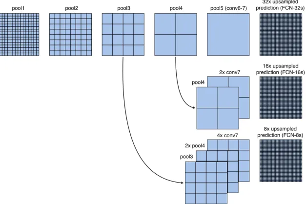
For the task of image segmentation, global information contains semantics of the whole image and local information indicates specific location of each object. In order to obtain accurate segmentation map, it needs the cooperation of coarse, deep, semantic information and fine, shallow, local infor-mation [95]. FCN introduces skip layer (or skip connection) to accomplish that. Fig. 10 describes the skip layer used in FCN. In general, it up-samples feature maps from different deep layers with different scales, then add with feature maps in shallow layers, in this manner, the predictions can combine both global and local information.

2.3.2

U-Net

U-Net [120] is a popular segmentation network specially designed for medical imaging which is built upon FCN [95]. The detailed architecture of U-Net is shown in Fig. 11, it consists of a down-sampling (contracting) path and an up-sampling (expanding) path, this kind of architecture is also known as encoder-decoder. In the down-sampling path, image representations are extracted with successive convolution and pooling operations at different scales. After each down-sampling operation, the number of image features is doubled. In total, the down-sampling path has 5 convolution blocks with each has two 3×3 convolution layers with ReLU activation, followed by a max-pooling with

pool1 pool2 pool3 pool4 pool5 (conv6-7) 2x conv7 pool4 4x conv7 2x pool4 pool3 32x upsampled prediction (FCN-32s) 16x upsampled prediction (FCN-16s) 8x upsampled prediction (FCN-8s)

Figure 10: The skip connections in FCN. Pooling layers and prediction are shown as grids, convolu-tion layers are omitted for clarity. Image is from [95].

stride 2×2 operation except the last block which is also called bottleneck block. While in the up-sampling path, the purpose of it is to recover resolution of the contextual information extracted from the down-sampling path and enable precise localization by utilizing the local information. Deconvolution operation with stride 2×2 is applied to up-sample the feature resolution, then concatenate with the features that have the same dimension from the down-sampling path, this is the skip connection in U-Net. After concatenation operation, two 3×3 convolution layers with ReLU activation are used to reduce the number of feature maps. Finally, a 1×1 convolution [93] is used to map the features to the desired number of segmentation classes.

In conclusion, U-Net has two major differences compared to FCN. Firstly, the architecture of U-Net is symmetric, it has a u-shaped structure. Secondly, U-Net applies concatenation operation instead of summation operation in FCN to fuse feature maps in skip connection. And the skip connection (or skip layer, residual connection [59]) in a CNN is extra connection between different layers that skips one or more layers.

The Overlap-tile Strategy

The resolution of medical image sometimes is extremely large. It’s very challenging for training deep network with such large input images even with a modern GPU. U-Net [120] introduces a seamless patching strategy - the overlap-tile strategy. Basically, the whole image is divided into patches and

Figure 11: The U-Net architecture. Image is from [120].

all the patches are predicted one by one. In order to obtain prediction of a small part, we need image data from an area which is much more bigger than the small part of the input image. The explanation of this strategy is shown in Fig. 12. The area in green line of the input image is predicted using the area in blue line as the input. Image data is extrapolated by mirroring at image boundary.

Figure 12: The Overlap-tile strategy. Left image is input image and right image is the corresponding segmentation mask. Images are from [107].

Chapter 3

Lung Segmentation in Chest X-ray

by Fully Convolutional Networks

This chapter will present the first work of this thesis, the lung segmentation in chest X-ray by fully convolutional networks.

3.1

Introduction

A variety of imaging techniques are now available in the medical diagnosis field, such as X-ray imag-ing, computed tomography (CT) and magnetic resonance imaging (MRI). Despite the higher precise and sensitivity of CT and MRI, traditional X-ray imaging is still the most commonly used technique in medical diagnostic examinations and lung examinations because of less radiation dose and low cost. Chest radiography, as a cost-effective procedure and most widely used imaging techniques, is account for about one-third of all radiological procedures [141]. It provides a powerful tool to study various structures inside the thoracic cavity. Therefore chest radiography is widely used for the diagnosis of several diseases in clinical practices including emphysema, lung cancer and tuberculosis. Since the information extracted directly from lung regions such as size measurements, irregular shape and total lung volume can provide clues about early manifestations of life threatening diseases like emphysema [33, 103], pneumothorax, cardiomegaly and pneumoconiosis, accurate segmentation of lung regions in chest X-ray is a primary and fundamental step in computer-aided diagnosis (CAD) and plays a vital role for subsequent medical image analysis pipeline.

There are a number of difficulties and challenges for accurate lung segmentation in chest X-ray images. First of all, the shape and appearance of lung is greatly diverse due to differences in gender, age and health status. Secondly, the existence of external objects such as sternal wire, surgical clips and pacemaker will further makes the lung segmentation task much more difficult. Finally, some anatomical structures of lung may cause hardness for segmentation. For instance, the strong edges of the ribs and clavicle regions lead to local minima for many minimization methods.

3.2

Method

Most of the traditional segmentation methods for lung segmentation in chest X-ray rely on hand-crafted features. Recently, the progress of deep learning, especially CNNs based models have achieved huge success in many medical image analysis tasks.

In this study, we focus on applying robust deep CNN models to directly learn from image pixels for segmenting lung region in chest X-ray images. Specifically, we develop an automated framework based on FCN [95] and U-Net [120] for lung segmentation and demonstrates the superior performance of deep learning based approaches. Finally, we perform comparison study on 3 public chest X-ray image datasets to evaluate the performance of these models.

3.2.1

FCN

Since FCNs have 3 different architectures: FCN32, FCN16, FCN8, the only difference between these architectures is the skip connection. Specifically, FCN32 has no skip connection, FCN16 has one skip connection and FCN8 has two skip connections. In order to study the effect of skip connection, we adopt two FCNs for this study, FCN32 and FCN8. Following will give some details of these two architectures.

The architecture of FCN32 is shown in Fig. 13. It has five pooling layers, so the dimension of input image will be reduced to ₃₂1 of the original input size, e.g. for an input image with size 512×512, the size in the smallest scale with be 16×16. Every level in FCN32 has two 3×3 convolution followed by ReLU activation except the last level. For the last level, it uses a 7×7 convolution with ReLU activation. After the 7×7 convolution, two 1×1 convolution with ReLU are used. Finally, it directly uses a transposed convolution with stride 32×32 to up-sample the 16×16 feature maps back to the original size, i.e. 512×512. Since the up-sampling rate is 32x, this type of FCN is called FCN32.

The architecture of FCN8 is shown in Fig. 14. Same with the FCN32, It also has five pooling layers. The major difference of FCN8 compared with FCN32 is that it uses feature addition operation to merge features in the previous layers. More specific, it firstly uses a transposed convolution with stride 2×2 to up-sample the 16×16 feature map back to 32×32, then a 1×1 convolution with ReLU is applied on the previous features map after the fourth pooling operation which has the same size 32×32, then uses addition operation to add these two feature maps with size 32×32. After addition operation, another transposed convolution with stride 2×2 is applied on the result feature maps. The feature map now has resolution 64×64, then add with another 64×64 feature map which is obtained from 1×1 convolution on the previous features after the third pooling operation. Finally, a transposed convolution with stride 8×8 is applied on the result feature after addition operation to obtain the final 512×512 segmentation map.

3.2.2

U-Net

The detailed network structure of U-Net is shown in Fig. 15. It is identical with the U-Net except for only one difference, in this study, we use convolution with padding instead of convolution without

Conv 3 × 3, ReLU Max-pooling 2 × 2

Up-conv 32 × 32 Conv 1 × 1, ReLU Input image tile

Output segmentation map

Conv 7 × 7, ReLU 512 × 512 256 × 256 128 × 128 64 × 64 32 × 32 16 × 16 64 64 64 128 128 128 256 256 256 512 512 512 1024 1024 1024 2048 2048 2 2 512 × 512

Figure 13: The architecture of FCN32 used in this study. Blue boxes represent image features. The number of features is indicated on the right of the box. The resolution of each level (features have the same resolution) is indicated on the left side of each level.

padding in the original U-Net. Therefore there is no dimension lose after every convolution operation.

3.3

Experimental Results

3.3.1

Datasets

Three publicly available datasets are used to evaluate the performance of different methodology in this study.

Conv 3 × 3, ReLU Max-pooling 2 × 2

Up-conv 2 × 2

Conv 1 × 1, ReLU

Input image tile

Output segmentation map

Conv 7 × 7, ReLU 512 × 512 256 × 256 128 × 128 64 × 64 32 × 32 16 × 16 64 64 64 128 128 128 256 256 256 512 512 512 1024 1024 1024 2048 2048 2 2 2 2 2 Up-conv 8 × 8 Addition 2 2 2 512 × 512 64 × 64 32 × 32

Figure 14: The architecture of FCN8 used in this study. Blue boxes represent image features. The number of features is indicated on the right of the box. The resolution of each level (features have the same resolution) is indicated on the left side of each level.

Montgomery County (MC) Dataset

The MC dataset [69] is from the department of Health and Human Services, Montgomery County, Maryland, USA. It contains 138 frontal chest X-ray images, among them 80 images are normal cases while 58 images are abnormal cases (i.e. tuberculosis). All images are provided in PNG format as 12-bit gray-scale images. The resolution of these images are either 4020×4892 or 4892×4020. The corresponding manual lung segmentation mask images are performed under the supervision of a radiologist.

1 64 64 128 64 64 2

Conv 3 × 3, ReLU

Copy and Concat

Max-pooling 2 × 2 Up-conv 2 × 2 Conv 1 × 1, ReLU 128 128 256 256 512 512 1024 1024 512 512 256 256 128 Input image tile Output segmentation map 512 × 512 256 × 256 128 × 128 64 × 64 32 × 32

Figure 15: The architecture of U-Net used in this study. Blue boxes represent image features. The number of features is indicated on top of the box. The resolution of each level (features have the same resolution) is indicated at the bottom left of each level.

Shenzhen Dataset

The Shenzhen dataset [69] is from Shenzhen No.3 People’s Hospital, Guangdong Medical College, Shenzhen, China. It consists of 662 frontal chest X-ray images in total, 326 images are normal cases while 336 images are abnormal cases. These images are also stored in PNG format and the resolution of them are vary but roughly 3000×3000. The corresponding lung segmentation masks are provided by [131]. However, for Shenzhen dataset, only 566 images have the corresponding manual lung segmentation mask images. Therefore only 566 images in this dataset are actually used for this study.

Japanese Society of Radiological Technology (JSRT) Dataset

The JSRT dataset [126, 142] is collected from 14 medical centers in Japan. It has 247 chest X-ray images, among them 93 images are normal cases and 154 are abnormal cases. All images are in PNG format and having 12-bit gray-scale with resolution 2048×2048. All the associated manual lung segmentation mask images are also available.

Three example chest X-ray images and their corresponding lung segmentation masks are shown in Fig. 16.

In addition, in order to evaluate the generalization ability of each segmentation model, we further merge all the 3 datasets which we call it Combined dataset in this study.