School of Social Sciences
Economics Division
University of Southampton
Southampton SO17 1BJ, UK
Discussion Papers in
Economics and Econometrics
A Model of Credit Limits and Bankruptcy
with Applications to Welfare and
Indebtedness
Xavier Mateos-Planas
No. 0910
This paper is available on our website
http://www.southampton.ac.uk/socsci/economics/research/papers
with applications to welfare and indebtedness
Xavier Mateos-Planas∗
Economics Division, University of Southampton, U.K. First version September 2006
Current version April 2008
Abstract
This paper presents a macroeconomic model of unsecured consumer debt and default where credit conditions consist of pre-approved interest rates and borrowing limits, a feature of actual credit cards. All loans, irrespective of their size and risk, take place against the same type of credit line, and some borrowers are credit constrained. This type of situation is shown to arise in a free-entry competitive equilibrium if there are fixed costs in banking and the banks’ decisions on interest rates and on credit limits are made separately. Numerical experiments are conducted to study, on one hand, the macroeconomic and welfare effects of the consumer bankruptcy code, and on the other hand, the consequences of various factors for both indebtedness and bankruptcy. Restricting bankruptcy filings – be it through a stricter Chapter 7 means testing or a longer period of credit exclusion – leads to sizable welfare loses. The recent rise in filing rates and debt is best explained by a combination of lower intermediation costs and more severe non-discretionary expenditures shocks. The endogenous response of the credit limit proves to be crucial for these findings.
1
Introduction
Borrowing limits are one defining feature of the pre-approved credit lines that characterise credit-card unsecured consumer loans. Card issuers offer a limit rather than a specific loan size. There is good evidence that these limits are effective and have a substantial effect on consumer’s borrowing and consumption choices.1 There are also indications of interactions between these credit limits and default risk. Credit limits may respond to default-risk con-siderations since banks will be more cautious in their lending when failure is more likely.2
∗
Email: [email protected]. This research has been funded by the ESRC (U.K.) through grant RES-000-22-1149. Much of it was conducted while at the Department of Economics of SUNY at Stony Brook. Versions of this paper have been presented at the University of Pennsylvania, the winter meetings of the AEA Chicago 2007, the EEA Congress Budapest 2007, City University London, and the Royal Economic Society Conference 2008 Warwick. Thanks for comments to Irina Telyukova and Makoto Nakajima on an earlier version. Comments by D. Krueger, V. R´ıos-Rull and M. Tertilt have proved particularly helpful. All responsibility for mistakes is of course only mine.
1Gross and Souleles (2002) and Cox and Jappelli (1990) estimate a considerable effect of removing credit
limits on levels of debt.
2
This view receives support in Gross and Souleles (2002b) and Dey and Mumy (2005) finding that larger credit lines are associated with less default. The Federal Reserve (2003) recognises that lenders adjust credit limits on account of perceived creditworthiness.
Is the interplay between credit limits and other variables of practical consequence? In par-ticular, is it significant in order to understand the causes of the rise in both bankruptcy and debt since the early 1990’s, as well as the impact of related policy actions?
The general aim of this paper is to take a step towards the study of the macroeconomic positive and welfare effects of various factors – such as the bankruptcy code, household risk, the costs of intermediation, or the stigma of bankruptcy – when both the borrowing limits on credit lines and the risk of bankruptcy can respond jointly. The first objective of this paper is, accordingly, to present a macroeconomic model of unsecured consumer debt that can be used to study the determination of the credit limits on contracts that resemble actual credit lines. The model pursues to accommodate the observation that a particular type of credit line is used to different degrees by different borrowers, so contracts with the same pre-approved interest rate and credit limit are used as the vehicle for loans of varying size and, hence, risk.3 This is in general an anomaly for the view that financial markets are fully competitive and frictionless and, therefore, achieving this paper’s first objective calls for finding suitable departures from that standard model. The second, more applied, objec-tive is to start assessing the practical significance of the response of the borrowing limits for the effects studied. First, I consider changes in the conditions for bankruptcy in the form of a stricter means test and a longer period of exclusion from credit after filing.4 Second, I explore the plausibility of different explanations for the rise in default and personal debt in the U.S.
I use a version of the standard macroeconomic model of capital accumulation, endogenous labour supply, and idiosyncratic risk with incomplete markets of the kind proposed by Aiya-gari (1994). Individual risk is caused by random shocks to labour productivity and shocks to liabilities. The latter consist of non-discretionary expenditures associated with bad luck, including medical and legal bills, and other unintended disruptions. In order to partially insure consumption, besides saving in a riskless bond, households can borrow against any credit line in the set of actively traded contracts, each defined by a non-contingent interest rate and a credit limit. The absence of enforcement implies the possibility of default on debt. The set oftradedloan contract types and the default decisions are determined jointly in equilibrium. Individual households decide whether to declare bankruptcy and see their debts discharged within a setting that encompasses the main provisions in Chapter 7 of the U.S. bankruptcy code and the practice of restricting credit access to borrowers with poor credit scores. On its part, a bank can choose to offer any type of credit line from within a specified set of available ortradeablecontracts. The extent of competition in intermediation is shaped by the specific restrictions described by this tradeable set, to which I turn now to.
The contracts take the form of pre-approved one-period credit lines that a particular bor-rower may or may not use in full, and do not (or cannot) screen a borbor-rower’s individual characteristics beyond their bankruptcy status. Therefore this setting might in principle accommodate the situation characteristic of the credit-card industry where loans of different
3
The evidence in Edelberg (2003, Table 12) suggests that for unsecured general consumer loans, credit card loans, and education loans, the loan balance does not appear to be significant for the interest rate. Thus the assumption made here to study the unsecured credit market need not be grossly misleading.
4
In the U.S, the recent Bankruptcy Act 2005 considerably tightens up the conditions and process for the discharge of debt under Chapter 7.
size and risk take place under the same interest-rate and credit-limit conditions – a case of adverse selection of the type documented in Ausubel (1991). But this is by no means a necessary outcome. Standard free-entry competition could still result in contracts with dif-ferent limits and interest rates serving each level of individual borrowing like in Chatterjee et al. (2007), thus rendering superfluous the distinction between the credit limit on a credit line and the value of the loans taken against this credit line. In order for meaningful credit limits to arise, this paper will have to make some specific assumption regarding the banking industry. First, there are fixed costs to processing a credit line. A fixed cost may create a competitive advantage for banks extending longer credit limits even if they incur a higher risk. The fixed cost however is assumed to vary with the interest rate to reflect the traded values within each price segment of the industry, so similar scale effects are ruled out across banks competing in price. Second, in the interest of tractability, there is a particular form of competition in banking. The set of tradeable contracts is restricted so that banks cannot compete simultaneously in both the credit limit and the interest rate. This is as though the bank consists of two separate arms for the price and the quantity decisions which play a Nash equilibrium.
The analysis can focus, given those assumptions, on stationary equilibrium outcomes where only one type of credit line turns out to be traded. For each individual state, there is a threshold level of debt above which household default occurs. The prevailing credit limit expresses a balance between the cost advantage of larger loans against their higher default risk. Credit is thus extended by the banks only as far as it does not exceed the house-hold debt threshouse-hold associated with states which will happen with too high a probability. Although loans of different size command a different risk and there may be borrowing con-strained households, potential entrant banks do not find it profitable to deviate by offering either different loan limits or a lower interest rate. Establishing this result requires studying the consequences of entry decisions of intermediaries across the tradeable credit lines and the reaction of households when presented with such off-equilibrium deviations, which, to my knowledge, this paper does for the first time. To facilitate the argument, I first define a pre-entry equilibrium for a given single borrowing limit, next I study the determination of the credit limit in apost entry equilibrium when there is free entry at the given interest rate, and, finally, I study conditions for such post-entryequilibrium to survive when there is price competition.
The model is calibrated to match features of the U.S. economy, including figures for default. This setting satisfies the conditions identified earlier for a single credit line to be supported in equilibrium. The optimal credit limit coincides with the level of debt above which a certain sizable (i.e., high probability) type of households would start defaulting. In the benchmark model, bankruptcy occurs only for low-productivity bad-luck individuals with sufficiently high debts. The effect on the stationary equilibrium of changes in parameters is investigated numerically. A stricter means test and a tougher punishment of bankruptcy both imply an aggregate welfare loss. Much of this welfare impact is driven by the impli-cations of the subsequent loosening of the credit limit. Utility declines most for bankrupt individuals and a looser credit limit shifts the distribution of agents towards the high-debt bankruptcy region. As for the recent rise in bankruptcy, a more severe expenditure shock is a prime candidate explanation, as opposed to the entrenched notion of a fall in the stigma cost. Only the former change can, in combination with the appropriate reduction in bank-ing intermediation costs, be consistent with the observed increase in levels of personal debt
andthe rise in the average amount of debt discharged during bankruptcy, and the observed extension of credit limits. The endogenous loosening of the credit limit – also a feature in the data – is essential for the latter.
This paper is a contribution to the recent literature analyzing bankruptcy and credit in quantitative general equilibrium models. At the methodological level, its most distinctive features are the consideration of loans with different size and risk taken against the same credit line, and the joint determination of the credit limit and default risk under competi-tion. In Mateos-Planas and Seccia (2006) the credit limit is endogenous, but positive default cannot arise in equilibrium. The approach in C´arceles-Poveda et al. (2007) is similar. Li and Sarte (2005) and Athreya (2002) can be seen as having also a single credit line and adverse selection, but the borrowing limit is set exogenously and the outcome will generally fail to stand under free-entry competition in banking. In a way, the present paper investi-gates which conditions can reconcile the type of arrangement characteristic of these papers – and more generally those in the class of Aiyagari (1994)’s – with the optimal lenders’ choices in equilibrium. Chatterjee et al. (2007) use a similar model but under the standard assumption of full price competition without intermediation fixed costs. As a result, there is a full menu of lending interest rates which depend on the loan size and the borrower’s individual characteristics. In the present paper’s language, it is as though each credit line is used to the full extent of its approved credit limit, and, consequently, the observable distinction between credit limit and credit balances (e.g., Gross and Souleles 2002) becomes immaterial.5 This might not provide a fully accurate description for the pricing of credit cards though. Note that this is in spite of the growing importance of risk-based pricing for the setting of interest rates. This practice involves the use of credit scores on individual financial histories but, once a credit line is approved, the interest does not depend on the amount borrowed.6 In the models of the literature, including the present one, credit scores
are the same for all agents with access to credit and thus a single lending rate seems defen-sible. On this front, the significance of the present paper is that it reconciles the emergence of positive default with this realistic outcome for the pricing of loans.
At the level of substantive results, one contribution of this paper is to add new insights into the long-run welfare consequences of the bankruptcy setting. It finds a substantial negative impact of a stricter means test. In contrast, Chatterjee et al. (2007) find a sizable increase in welfare (although the design of their experiments accounts for transitional effects and may not be directly comparable). In Li and Sarte (2005) there is also a decline in welfare with given borrowing limits but a Chapter 13 option for debt repayment. Athreya (2002) finds negligible effects of the mean test. The present paper finds that a longer duration of the punishment for bankruptcy is clearly detrimental to welfare, whereas Chatterjee et al. (2007) find otherwise. Another contribution is the interpretation of recent developments in debt and default. Athreya (2004) has attempted to study recent changes in default and indebtedness using a model that shares many features with Chatterjee et al. (2007). Al-though some of his basic conclusions seem to follow here as well - such as the need of more than one explanatory factor, including innovation in banking- the type of shocks in the mix differ. Livshits et al. (2006) have recently undertaken a more thorough quantitative exploration with the same type of model. They find a fall in the stigma to bankruptcy must
5Athreya and Simpson (2006) and Livshits et al. (2007) share similar features.
6
have played an important part. The present paper also assesses alternative explanations against the evidence, and reaches conclusions more supportive of the expenditure shocks as the cause of rising bankruptcy. A stigma shock counter-factually reduces the credit limit.7 The rest of the paper is organised as follows. Section 2 presents the model. Section 3 defines the equilibrium and discusses the conditions for only one type of credit line to arise. Section 4 presents the benchmark calibration. Section 5 studies changes to the bankruptcy setting. Section 6 studies explanations for observed rises in default and indebtedness. Section 7 concludes.
2
Model
This paper studies a production economy with incomplete markets and default risk. Debt repayments cannot be enforced and default occurs under a bankruptcy code which resembles Chapter 7 in the US. Competitive financial intermediaries offer credit lines specifying a maximum borrowing limit, there is fixed cost to each credit contract, and there may be conditions on the form of competition in intermediation.
2.1 Individual households
There is a continuum of individual agents with total mass equal to one. Each agent has a unit endowment of time per period which can be divided between leisure lt and working in the market 1−lt. Since labour supply is divisible,lt∈[0,1]. An agent’s labour productivity in the market st in any period can take on two values s1 and s2 with s1 > s2. This pro-ductivity is stochastic and follows a Markov process with stationary transition probabilities
πs(s0 |s) for s0, s∈ {s1, s2}. These probabilities are independent across individual agents. Each efficient unit of labour earns a market wage ratew. An individual agent with a clean bankruptcy record can also face an independently distributed expenditure, or liability, shock
xt ∈ {x1, x2} with x1 < x2. A realisation xt has probability πx(xt). To simplify, agents with a bankruptcy flag cannot experience the high liability shock since they may not be able to afford it.
An agent in period tcan trade one-period contracts in financial markets to an extent that depends on her bankruptcy state, which is denoted by zt ∈ {0,1}, and her bankruptcy decision, dt ∈ {0,1}. An agent with zt = 0 and dt = 0 has a clean bankruptcy record and can save and borrow at the market interest rates. The interest rate on savings is denoted byrt+1. Borrowers can choose any type of contract among a set of traded credit lines. Each
type of contract specifies a borrowing limit and interest rate. More specifically, a credit line type is characterised by a valueb? ≤0 such that debt cannot exceed (−b?), and the associ-ated borrowing-deposit spreadλ? sort+1+λ? represents the interest rate on this loan. The
set of traded contracts (b?, λ?) available to the household is denoted by Ωt+1.8 There is also
an inconsequential upper bound on assetsb >0. Ifzt= 1, it is said that the agent bears a bankruptcy flag which prevents her from borrowing and sets a cap on the amount of bonds
7
Narajabad (2007) has also focused on the determination of credit limits to assess alternative explanations. In spite of the substantial differences in the formal approach, it also finds that the stigma hypotheses may be problematic when credit limits are endogenous.
8Thus attention is restricted to contracts where the promised delivery – in the language of Dubey et al.
she can hold given by the asset exemption level bex ≥0. If zt = 0 and dt = 1, the agent is said to file for bankruptcy. In this filing period the agent is unable to either borrow or lend. An agent with a clean record, i.e. zt= 0, may decide either not to repay her negative bond balances and non-discretionary expenses at any time by making the default (or bankruptcy) choice dt = 1 or, otherwise, remain clean by choosingdt= 0. In the former case, the indi-vidual will bear the bankruptcy flag in the next periodzt+1= 1, in subsequent periods there
is a probability ρ that she will loose the bankruptcy flag. This default option is available only as long as the current normalised pre-tax labour earnings do not exceed a specified means test levelmtest≥0, or (1−lt)st≤mtest.
Preferences are defined over stochastic processes for consumption,ct, and leisurelt. Default-ing or remainDefault-ing bankrupt carries a non-pecuniary stigma or disutility cz >0 per period. These preferences can be represented by the utility function
E ∞ X t=0 βt 1 1−σ cηtl1t−η 1−σ −cz(dt+zt)
where η∈[0,1], σ >0, β ∈(0,1), and E is the expectation operator. Note thatdt and zt cannot be both positive in the same period.
2.2 Intermediation
Borrowing and lending between any two consecutive periodstandt+ 1 take place through two-period lived intermediaries. Although in this section I will drop time indexes, it must be understood that quantities and prices are datedt+ 1.
A bank offers credit lines with a particular limitb? and interest spreadλ?. The associated interest rate, r +λ?, does not vary with the ex-post size of the loans taken against any credit line of this type. This arrangement intends to describe actual credit card contracts where banks have the possibility not to engage in individualised lending and, instead, set a pre-approved interest rate and maximum amount which a particular borrower may or may not use in full.9
At the time of issuing a particular credit line contract, the bank does not observe the bor-rower’s type and offers credit randomly to a representative section of the population, hence not knowing the amount that ex-post each will borrow and repay against that credit line. The bank then withdraws credit facilities from all those who default on past debts (i.e., who choosed= 0), or who have a bad credit record (i.e.,z= 1). Therefore all of the contracts of type (b?, λ?) are ex-ante identical, with the same average face value, denoted by L(b?, λ?), and default-adjusted non-recoverable value, denoted byLd(b?, λ?). There is a fixed cost to each credit line that depends on the interest rate,cF(λ?), which the bank incurs regardless of the amount lent (including zero). This can create a scale effect across banks competing in the credit limit, but not necessarily when competing in the interest rate. I will assume
9
In other papers, like Chatterjee et al. (2007), banks directly choose the size of the loan they wish to offer, thereby ruling out the constant-interest pre-approved credit lines of this paper. Note however that, without further conditions, the present assumption is still perfectly consistent with their outcome.
that this fixed cost is determined externally as a proportion cF of the average promised delivery on the loans offering that same interest rate.
In any given period, consider a bank extending a numberM of credit lines of type (b?, λ?) and investingKin risk-free productive capital. The bank thus takes deposits in the amount
M L(b?, λ?) +K. In the next period, the bank has to pay the interest on these deposits plus the fixed cost per credit line,cF(λ?), which amounts to a total cost of (1 +r)(M L(b?, λ?) +
K) +M cF(λ?). The revenues to the bank consist of the risk-free return on investment and the payments collected on the value of loans that are repaid, which amounts to a total revenue (1 +r)K+ (1 +r+λ?−cb)M(L(b?, λ?)−Ld(b?, λ?)), wherecb is the variable cost to (good) loans. So the bank net cash flow on each of theM contracts issued can be expressed as:
CF(b?, λ?)≡(λ?−cb)L(b?, λ?)−(1 +r+λ?−cb)Ld(b?, λ?)−cF(λ?) (1) Banks are competitive and take as given in (1) the pattern of fixed costs, and the average loan face and defaulted values associated with different types of contracts. Given this information, and for any measure of contracts, the bank seeks to maximise its net cash-flow by choosing which type of credit line to offer within the set of tradeable lines Ω.pThis tradeable set is exogenous to the bank and will be specified later with the equilibrium concept. In an equilibrium there is a set of actively traded credit lines Ω⊂Ω. Since there is free entry in traded lines, all credit lines in this set must make zero profits. Another requirement is that a bank offering a credit line not in Ω would make loses so there are no profitable one-period deviations. Formally, for all (b?, λ?)∈Ω:
CF(b?, λ?) = 0 if (b?, λ?)∈Ω (2a)
CF(b?, λ?) < 0 if (b?, λ?)∈/ Ω (2b)
2.3 Firms
Aggregate output is produced by firms that combine labour services N and capital K as inputs into a neoclassical production function. The production function is Cobb-Douglas with α the capital share. This output can be consumed, purchased for non-discretionary expenses and banks’ fixed costs, and invested in capital. The rate of depreciation of capital isδ.
Firms in the non-discretionary liability sector produce services out of final output goods by the amount of the expenses x. The price of the services provided adjust to guarantee zero profits, taking into account the fact that bills by those with negative debt who default or have a default flag will go unpaid. This crude setting rules out any feed-back effect of this price on the economy.
3
Equilibrium
The equilibrium concept is perfect competition, with price-taking optimising households, firms and intermediaries, and free entry in the markets for all tradeable loans in Ω. The set of credit lines that will effectively be traded, Ω⊂Ω, is a variable of central interest. In equilibrium, this set is determined so that, taking the households’ reactions into account, a bank does not find it profitable to deviate from it by introducing a new credit line (i.e.,
with different limit and/or interest) drawn from the tradeable set Ω. An equilibrium can thus be found in two steps. First, for a particular guess about the credit limits associated with the traded contracts, one can find allocations and prices, including the lending inter-est rates and hence the traded set Ω itself, that clear all markets and satisfy the banks’ zero profit condition (2a). I call this outcome apre-entryequilibrium.10 Second, given the conditions of bank competition described in Ω, one has to verify that profitable deviations in intermediation away from the traded set Ω can be ruled out in the sense of (2b). If this is the case, thepre-entryequilibrium will also characterise a post-entry equilibrium.
For tractability reasons, attention is focused on situations where there is a single type of credit line (b, λ,) being traded in equilibrium as the only element of Ω. One can first char-acterise the pre-entry equilibrium, including λ, associated with one particular credit limit
b, and then check that it corresponds to a post-entry equilibrium by ruling out feasible deviations away from (b, λ,) within Ω. The gist is to find conditions that may result in a single type of credit line being traded in (a post-entry) equilibrium. To this end, I will explore assumptions on the set of available deviation contracts, Ω.11
In particular, I will consider the case for a post-entryequilibrium where bank competition is permitted separately in the credit limit for the given interest rate and in the interest rate at the pre-entry limit, but not in both the limit and the interest rate simultaneously. That is:
Ω ={(b?, λ?) : (b?, λ?)∈(b× R+)∪(R−×λ)}
This constraint can be decentralized as the outcome of a Nash equilibrium between two decision makers within the bank, one of them setting the interest and the other setting the limit. This assumption will afford the sought tractability since it will result in a single type of contract being traded.12
The rest of this section proceeds as follows. First, it considers a pre-entry equilibrium for a single credit limit and discusses the default decisions. Then it considers the determination of the equilibrium credit limit in the post-entry equilibrium. Properties will be discussed first under general assumptions and then they will be applied to the specific kind of situation that will be relevant in the quantitative experiments. Finally, it turns to study post-entry competition in the interest rate.
3.1 Pre-entry equilibrium: one given credit limit
Consider one given constant credit limit b. This paper studies situations where the in-terest rates and credit limit are constant over time. The individual state space is S ≡ < × {s1, s2} × {x1, x2} × {0,1} with elements (b, s, x, z) ∈ S and AS its Borel σ-algebra.
10
This is the type of equilibrium situations studied in Li and Sarte (2005) and Athreya (2002).
11
With no fixed costs and unrestricted tradeable set – that is,cF = 0 and Ω =R×R – one would be in
a case analogous to Chatterjee et al. (2007). The configuration of the industry would be characterised by credit limits matching each level of individual borrowing. All borrowers fully use their chosen credit limit thus rendering superfluous the distinction between the limit offered on a credit line and the value of the loans taken against that credit line.
12
With simultaneous choices, credit lines with limits still arise but it becomes harder to establish conditions for a single contract.
The aggregate state then consists of a probability measure Φ over S that describes the distribution of individual types. In a stationary equilibrium this distribution must be con-stant. A stationary pre-entryequilibrium associated with bcan be formulated recursively. Given the parameters, apre-entryequilibrium is a probability measure Φ on the measurable space (S,AS), a deposit interest rater, a wage ratew, a lending spread λ, a value function
v(., ., ., .), decision rules for bonds b0(., ., ., .), leisure l(., ., ., .), and defaulting d(., ., ., .), and the face value and defaulted value of loans,L(λ, b) andLd(λ, b), such that:
(i) Household choices: Givenr,λ,wandb, the functionsb0(., ., ., .),l(., ., ., .),d(., ., .) and
v(., ., .) solve the problem
v(b, s, x, z) = max b0,l,du(c, l, z, d) +β X s0∈{s 1,s2} X x0∈{x 1,x2} πs(s0|s)πx(x0)v(b0, s0, x0, z0) s.t. d∈ {0,1}, d= 0 if s(1−l)> mtest b0+c= [(1 +r)b+ min{0, λb}](1−d) +ws(1−l)−x(1−d)(1−z) b0 ∈ [b, b] if z= 0 and d= 0 0, bex] if z= 1 {0} if z= 0 and d= 1 z0 =
0 if z= 0 and d= 0, or if z= 1 with prob. ρ
1 if z= 0 and d= 1, or if z= 1 with prob. 1−ρ
(ii) Firm behaviour: Givenw and r,w= (1−α)(K/N)α and r =α(K/N)α−1−δ. (iii) Market clearing:
Z S bdΦ = K Z S (1−l(b, s, x, z))sdΦ = N
(iv) Stationary distribution:
Φ(A) =
Z
S
Q(s, A)dΦ for A∈ AS,
withQ:S× AS →[0,1] being the transition function derived from the decision rules
b0,l and d, and the transition probabilities πs andπx.
(v) Banking - zero profits: Givenλ,r,cF(λ),L(b, λ) andLd(b, λ), the zero-profit condition (2a), with (1), is satisfied for Ω ={(b, λ)}.
(vi) Consistency of bank’s beliefs: The valuesL(b, λ) and Ld(b, λ) are consistent with the equilibrium distribution of borrowers and their default policy function. The fixed cost is determined according to:
¯
This equilibrium yields the only traded contract (b, λ) – which fully describes the traded set Ω – that is consistent with an equilibrium where the given b is the only active credit limit. Conditions (i)-(iv) characterise an equilibrium for a given credit limit and spread. Condition (v) says that the spreadλis such that the bank satisfies the zero-profit condition (2a). Condition (vi) states that the bank’s beliefs are based on the household’s behaviour and distribution, and formalises the assumption made in section 2.2 about the fixed cost as an externality. The resulting pattern of default behaviour and the determination of the bank’s beliefs demand further discussion.
3.1.1 Default
The individual household default policy function d(b, s, x,0), in part (i) of the definition, will typically imply that bankruptcy occurs if and only if debt (−b) is above a certain threshold. The exact value of this threshold depends on the individual productivity and liability states, and can thus be written as b(s, x). Formally, d(b, s, x,0) = 0 if and only if
b≥b(s, x). Another property, which holds in all the applications explored, is that default for the lower productivitys2happens at lower levels of debt, orb(s1, x)< b(s2, x). Also, default is more likely when the expenditure shock occurs sob(s, x1)< b(s, x2). Therefore there are two possible configurations for the four values b(s, x) depending on whether b(s1, x2) is bigger or smaller than b(s2, x1). When b(s1, x2) > b(s2, x1), default happens for the high-liability shockx2 at all productivity levelssbefore it happens under the low-liability shock
x1 for any productivity s. In the contrary case that b(s1, x2) < b(s2, x1), default happens for the low-productivity shock s2 for all x before it happens under the high-productivity shocks1 for any x. Figure 1 depicts the latter configuration.
b(s1,x1) b(s1, x2) b(s2,x1) b(s2,x2) 0
Fig 1. Default thresholds
3.1.2 Loan size and default risk
In order to study the zero-profit condition for banks (2a), one needs to describe the face and defaulted values of loans described by the termsLandLd. Denote byπd(b0, s, x) tomorrow’s default probability assigned by the bank to an agent with current type (s, x) and borrowing
b0. Regarding the distribution of borrowers, denote byh(b0, s, x) the density of borrowers of type (s, x) who will borrowb0, forb0 ∈[b,0]. In order to account for the possibility of a mass point of borrowing constrained agents, let H(b, s, x) denote the mass of borrowers of type (s, x) who will choose exactlyb. These objects have to be consistent with the equilibrium Φ, b, and d(., ., ., .) andb0(., ., ., .), thus:
πd(b0, s, x) ≡ P
s0,x0d(b0, s0, x0,0)πx(x0)πs(s0 |s) h(b0, s, x) ≡ φ(b0−1(b0, s, x,0), s, x,0)
H(b, s, x) ≡ Φ((˜b,s,˜ x,˜ z˜)∈S :b0(˜b,˜s,x,˜ z˜) =b,s˜=s,x˜=x,z˜= 0)
where φ(.) is the density associated with the equilibrium distribution Φ, and b0−1(.) is the inverse of the household’s policy function. With these definitions, the face value of a credit line and its defaulted (or write-off) value can be written as follows:
L(b, λ) =X x,s (−b)H(b, s, x) + Z 0 b (−b0)h(b0, s, x)db0 , (4a) Ld(b, λ) =X x,s (−b)H(b, s, x)πd(b, s, x) + Z 0 b (−b0)h(b0, s, x)πd(b0, s, x)db0 . (4b)
3.2 Competition in credit limits
The pre-entryequilibrium yields a set consisting of one traded contract Ω ={(b, λ)}, for a given arbitrary limitb. A post-entryequilibrium determines a specific limit bso the condi-tions of thepre-entryequilibrium and, additionally, the condition (2b) ruling out profitable deviations by banks from this traded contract (b, λ) are satisfied. The tradeable set of fea-sible deviations Ω only allows for competition in the credit limit at the given interest rateλ. The no-deviation condition (2b) requires that b be such that it maximises a bank’s cash-flow defined in (1) given the interest λ. To make this operational, one needs to describe the values for the face and defaulted values of loans for various possible deviation limits,
b? 6=b. The argument invokes the optimality of the household off the equilibrium. A line with a tighter credit limit b? > b would feature zero lending on the mass of the borrowers who in equilibrium wish to borrow more than that, but will serve the rest of borrowers on the same terms. A line with a looser limitb? < bwould still serve on the same equilibrium terms all the loans below the equilibrium limit, but would be making larger loans to at least some of the agents that were constrained in equilibrium and to the households that may now decide to borrow more and switch away from defaulting. I use ˜h(b0, s, x) and
˜
H(b?, s, x) to describe the off-equilibrium distribution betweenb? andb, which must satisfy
˜
H(b∗, s, x) +Rb
b∗h˜(b0, s, x)db0 ≥ H(b, s, x) with equality for b? = b. The off-equilibrium
ex-ante loan face valueL(b?, λ) and defaulted valueLd(b?, λ) can be expressed:
L(b?, λ) = P x,s h R0 b?(−b0)h(b0, s, x)db0 i if b? > b P x,s h (−b?) ˜H(b?, s, x) +Rbb?(−b0)˜h(b0, s, x)db0 +R0 b (−b 0)h(b0, s, x) db0i if b? < b (4c) and Ld(b?, λ) = P x,s h R0 b?(−b 0)πd(b0, s, x)h(b0, s, x) db0i if b? > b P x,s h (−b?)πd(b?, s, x) ˜H(b?, s, x) +Rb b?(−b0)πd(b0, s, x)˜h(b0, s, x)db0 +Rb0(−b0)πd(b0, s, x)h(b0, s, x)db0 i if b? < b (4d) In these expressions, the off-equilibrium terms are determined by the household’s reaction to the availability of loans with a limit that exceeds the equilibrium−b. One wants now to establish whetherb maximises the bank’s cash-flow.
3.2.1 Bank cash-flow and the credit limit
In order to analyse the effect of a credit limit (−b∗) – possibly different from the given equilibrium one b– on the bank’s net cash flow (1), it will be useful to define the expected default probability among the marginal borrowers, or marginal default probability, as a function of b∗,M D(b∗), as follows: M D(b∗)≡ P 1 s,xg(b∗, s, x) " X s,x g(b∗, s, x)πd(b∗, s, x) # , (5a)
where, given the terms in (4), the composition of the marginal borrowers is described as
g(b∗, s, x)≡ h(b∗, s, x) when b∗ > b H(b∗, s, x) when b∗ =b ˜ H(b∗, s, x) + (−b∗) ˜∆(b∗, s, x) when b∗ < b (5b)
where the new mass of borrowers caused by a looser limit is the term ˜
∆(b∗, s, x)≡˜h(b∗, s, x) + d ˜H(b ∗, s, x)
d(−b∗) (5c)
This marginal default probability is in general discontinuous in the bank’s choice at the default breakpoints b(s, x) depicted in Figure 1, where the default probabilities πd shift, and at the equilibrium limitb, where the type-composition of the marginal borrowersg(...) switches. Elsewhere, it is continuous if the distribution is continuous, with the default terms
πd’s constant and variation, if any, caused only through the composition terms g(b∗, ., .)’s.
In spite of the discontinuities in the default probability, the bank’s objective CF(b∗, λ) in (1), remains continuous in the choice b∗ for all b∗ > b. For b∗ < b, the cash-flow is left-discontinuous at the default breakpoints b(s, x) where, because of the higher default risk on the mass of borrowers at the credit limit, the cash-flow drops with a larger limit (−b∗). For values of b∗ other than oneb(s, x) or b, the objective is differentiable, and the sign of the derivative of the cash flow with respect to the bank’s credit limit (−b∗) depends on the marginal default probability compared to the lending interest rate. At the existing limit
b, the cash flow shows a right-discontinuity in the bank’s choice b∗ since there the pool of borrowers who are credit constrained switches to this bank as the limit (−b∗) is increased. The sign of the jump depends again on the marginal default probability. There may also be a left-discontinuity atbwhen it coincides with one of the default breakpoints where, as just discussed, the cash-flow drops if (−b∗) is increased. This is proposition 1 (see Appendix for details).
Proposition 1. (Properties of the bank’s objective) Suppose that g(b0, s, x) is piece-wise continuous inb0.
(a) For b∗ > b, the bank’s cash-flow is continuous. For b∗ < b, it is left-discontinuous at default breakpointsb(s, x), where the cash-flow drops with (−b∗), or CF(b∗−0, λ)< CF(b∗, λ).
(b) The bank’s cash flow is differentiable inb∗ as long asb∗ 6=b(s, x) andb∗ 6=b
for all individual types (s, x). There CF(b∗, λ) increases with (−b∗) iff
λ−cb 1 +r+λ−cb
> M D(b∗).
(c) The bank’s cash flow has a right-discontinuity atb, where
CF(b, λ)> CF(b+ 0, λ) iff λ−cb 1 +r+λ−cb
> M D(b).
The bank’s cash flow has a left-discontinuity atbonly if b=b(s, x), where
CF(b−0, λ)< CF(b, λ).
In order to characterise the shape of the bank’s objective one needs to ascertain specific properties of the marginal default probability function,M D(b∗), in Eq.(5). Consider first a
b∗ 6=b. The marginal default probability as a function of the credit limit, (−b∗), increases discontinuously at the default break points b(s, x), as more events can lead to default and theπd’s increase. Between breakpoints, it changes only because of changes in the distribu-tion of the marginal borrowers across productivity levels, g(b∗, ., .). Second, consider now an increase in (−b∗) atb∗ =b. The discontinuous effect on the marginal default probability follows from the distribution describing the composition of the marginal borrower shift-ing. In the special case that b coincides with one of the default breakpoints, the upward shift in individual default probabilitiesπd will work to causeM D to jump. Therefore, the marginal default probability tends to be increasing in the limit (−b∗) as individual default probabilities rise, and only dramatic improvements in the distribution of the marginal bor-rowers could upset this pattern. I will make the assumption that, even if such swings in the distribution were to occur, the effect on the default probability would be limited.13
Assumption 1. The sign ofM D(b)−(λ−cb)/(1 +r+λ−cb) is increasing in (−b).
As a consequence of these properties of the marginal default probability, and the bank’s objective, one can establish necessary and sufficient conditions for the optimal bank choice of limit b∗ to coincide with the equilibrium value b. First, optimality of b requires that the cash flow there CF(b, λ) is not less than at some close tighter limit CF(b+ 0, λ). By Proposition 1(c) this requires the marginal default probability at this point M D(b) to be small enough relative to the interest spread. Under Assumption 1 about M D(.), this is also sufficient to guarantee that the cash-flow is smaller for any tighter limit (i.e. lower b∗) by Proposition 1(b). Second, it is also necessary that b coincides with one of the default breakpoints so that the cash flow displays for a slightly looser limit the drop described in Proposition 1(c). Otherwise, the cash-flow will increase continuously for some looser limit. For this to be also sufficient to rule out higher cash-flow values for any looser limit (i.e. lower
b∗) it is enough that the cash flow becomes decreasing in the credit limit (−b∗) according to the condition in Proposition 1(b). Proposition 2 states this result more formally.
13
A stronger assumption is that M D is increasing in (−b∗). But this can still be derived as a result
under plausible assumptions of the distributional shifts. Specifically, if there is a degree of persistence in productivity levels and the proportion of low-productivity borrowers increases (weakly) with levels of debt, it can be shown that the marginal default probability also increases (weakly) between breakpoints with the
credit limit (−b∗) Atb∗=bif, again, the proportion of low-income agents does not decrease, the marginal
Proposition 2. (Equilibrium credit limit) Suppose that g(b0, s, x) is piece-wise continuous inb0. Suppose Assumption 1 holds.
The bcharacterises the bank’s optimal choice of limit if:
(a) It coincides with a default breakpoint, so b=b(s, x) for some (s, x). (b) It is a local maximum in the sense that
M D(b−0)> λ−cb
1 +r+λ−cb
> M D(b) (6)
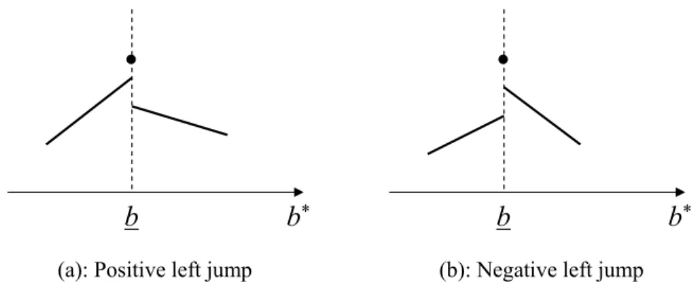
Essentially, in this proposition the bank’s cash-flow is single-peaked and two-side discon-tinuous at the equilibrium credit limit b. Figure 2 provides a visual representation of two cases consistent with Proposition 2.
(a): Positive left jump (b): Negative left jump
b
b
*b
b
*•
•
Fig 2. The equilibrium bank’s objective as a function of the bank’s choice of limitb∗.
3.2.2 A specific case
To characterise the equilibriumbusing the above result, one must verify that the marginal default probability in Eq.(5) satisfies Assumption 1. Thus further details would be needed about both the transition probabilities and default behaviour behindπd, and the equilibrium distribution underlying h and H. In particular, when the default probabilities πd change sharply enough for all income groups with the levels of debt, then the changes in income composition are of minor importance and then Assumption 1 holds. This is relevant because, as it turns out, in the applications studied in this paper, these type of conditions will be always satisfied. For concreteness, one can also focus on the situation when, as in the case depicted in Figure 1, the default behavior is such that b(s1, x2) < b(s2, x1). This is Proposition 3.
Proposition 3. (Characterisation) Suppose that g(b0, s, x) is piece-wise con-tinuous in b0. Assume a default pattern such that b(s1, x2) < b(s2, x1). The equilibrium credit limitb is determined as follows:
(a) b=b(s2, x2) if, for alls∈ {s1, s2},
0< λ−cb
1 +r+λ−cb
(b) b=b(s2, x1) if, for alls∈ {s1, s2},
πs(s2|s)πx(x2)< λ−cb
1 +r+λ−cb
< πs(s2 |s)
(c) b=b(s1, x2) if, for alls∈ {s1, s2},
πs(s2|s)< λ−cb
1 +r+λ−cb
< πs(s2 |s)(1−πx(x2)) +πx(x2)
(d) b=b(s1, x1) if, for alls∈ {s1, s2},
πs(s2 |s)(1−πx(x2)) +πx(x2)< λ−cb
1 +r+λ−cb
<1
As one runs over the possible default breakpoints from case (a) to case (d), the credit limit becomes looser. Case (a) is one where even the worst possible misfortune is too likely for all borrowers and, therefore, the borrowing limit is set so tight as to rule out default com-pletely. At the other end, in case (d) the probability of bad individual states is low and the chosen credit limit will therefore be loose enough to allow for default in all those rare states, preventing bankruptcy only in the highly probable good scenario of high productivity and low labilities.
The relevant quantitative benchmark will correspond to case (b) of Proposition 3. In this case, the probability that a borrower will transit into a state of low income and high non-discretionary liabilities is too low for the bank to tighten the credit limit in order to prevent default in that situation. On the other hand, the probability that any agent transits into a state of low income, regardless of the liability shock, is too high for the bank to per-mit default whenever this event happens. This leads the bank to choose the credit liper-mit at the level of debt where low income agent with low liabilities would start defaulting, or
b = b(s2, x1). With this limit, banks tolerate a positive default risk. Default will occur among low-productivity high-liability individuals since this is an event with a sufficiently low probability. More specifically, those who file for bankruptcy are low-productivity high-liability individuals with assets (i.e., negative debts) in the region [b, b(s2, x2)).
In this case, the borrowing constraint is determined by the incentives to default as repre-sented byb(s2, x1). However, exogenous factors that may affect the incentives to default will generally also have consequences for the relevant case through λ orr and might therefore alter the pattern of determination of the borrowing constraints according to Proposition 3. One can now motivate the role of the liability shock. If there is no high-liability shock, or πx(x2) = 0, then positive default - i.e. case (d) of Proposition 3 - will require that
π(s2 | s) < (λ−c
b)/(1 +r+λ−cb) at least for the good productivity s = s1. But this condition fails under the assumptions made in standard parameterizations for the house-hold’s income process and interest rates. Hence the need to include the liability shock so the analogous conditionπx(x2)π(s2 |s)<(λ−c
b)/(1 +r+λ−cb) can hold. In other words it makes the probability of the default state small enough that it pays to tolerate some of this risk.
One can also see why it is necessary to assume some fixed cost of intermediation cF >0. With the fixed cost in point (vi) of the definition, the zero-profit condition for the bank (2a) can be written as (λ−cb)/(1 +r+λ−cb) = Ld(b, λ)/L(b, λ) +cF. The default or write-off rate over total debt outstanding is necessarily smaller than the probability of de-fault for agents with debts in the dede-fault region, or Ld(b, λ)/L(b, λ)≤πx(x2)π(s2 |s). On
the other hand, we have seen that the existence of some default requires πx(x2)π(s2 |s)<
(λ−cb)/(1 +r+λ−cb). Therefore (λ−cb)/(1 +r+λ−cb) > Ld(b, λ)/L(b, λ) which is inconsistent with zero profits unlesscF >0.
3.3 Competition in interest rates
The scope for competition in banking is now extended to encompass competition in inter-est rates. Formally, banks can deviate from the one traded contract Ω = {(b, λ)} offering contracts with a different interest rate λ∗ at the given credit limit b. In the post-entry
equilibrium, no such a deviation can be profitable according to (2b). Clearly a deviation involving a higher interest rate λ? > λ will not be viable and can be ruled out. Consider now deviations involving a lower interest rateλ? < λ. Note that with adverse selection in default risk the standard argument to rule out such deviations from the zero-profit price does not carry over. The effect of different interest rates on the bank’s cash-flow (1) and the underlying household’s reactions have to be studied in greater detail.
By the assumption made earlier in section 2.2, the fixed cost associated with an interest rate
λ?, is determined by the promised deliveries on the contracts at that interest rate Formally,
cF(λ?) = cF(1 +r+λ? −cb)L(b, λ?). Therefore the sign of net cash-flow in (2b) can be written in terms of the interest rate, the default risk and the coefficient of the fixed cost. Ruling out deviations amounts to showing that this value is negative for all possibleλ? < λ. The following proposition states this more explicitly.
Proposition 4. (Ruling out deviations with lower interest) Consider a limit-only-competition post-entry equilibrium with λ and b. There are no profitable deviations withλ?< λiff
λ?−cb 1 +r+λ?−c b −L d(b, λ?) L(b, λ?) −cF <0 (7)
Since a lower interest comes with a lower default rate, the sign of the response of the left side of (7) toλ?is unclear. Studying this requires a more careful formalisation of the households’ choices and distribution dynamics off the equilibrium. Suppose a deviation contract (b?, λ?)
withλ? < λ is chosen by the individual borrower of type (b, s, x) withz = 0. The optimal
decisions are characterised by a value function ˜v(b, s, x|b?, λ?), decision rules for (price-adjusted) bonds ˜b0adj(b, s, x|b?, λ?), leisure ˜l(b, s, x|b?, λ?), and defaulting ˜d(b, s, x|b?, λ?) that solve the problem:
˜ v(b, s, x|b?, λ?) = max b0,˜l,d˜u(c, ˜ l,0,d˜) +βX s0,x0 πs(s0|s)πx(x0)v(˜b0adj, s0, x0, z0) s.t. d˜∈ {0,1}, d˜= 0 if s(1−l)> mtest b0+c= [(1 +r)b+ min{0, λb}](1−d˜) +ws(1−˜l)−x(1−d˜) b0 ∈ [b?, b] if d= 0 {0} if d= 1 ˜ b0adj = b0 b0 ≥0 b0(1 +r+λ?)/(1 +r+λ) b0 <0 z0 = 0 if ˜d= 0 1 if ˜d= 1
Note that ˜b0adj is adjusted so that the debt liability b0(1 +r +λ?) involves the deviation interest λ? but the continuation value can still be evaluated using the equilibrium value functionv built on λ.
The off-equilibrium distribution next period ˜Φ obeys ˜ Φ(A) = Z S ˜ Q(s, A)dΦ for A∈ AS,
with ˜Q:S× AS → [0,1] being the transition function derived the transition probabilities
πs and πx, and from the decision rules ˜b0adj, ˜l and ˜d. This distribution can be used to calculate in (7) the loan face value L(b?, λ?) and, with the equilibrium default rule d(...), the defaulted value Ld(b?, λ?), using expressions similar to (4) and settingb?=b.
Summing up, to find apost-entryequilibrium one can first rule out deviations in the credit limit using Proposition 3, and then verify there are no deviations in the interest rate ac-cording to Proposition 4.
4
Calibration
In the calibration parameters are selected so that an equilibrium matches certain targets and the outcome also corresponds to an equilibrium with banking competition by checking if the conditions in Propositions 3 and 4 hold.
The parameters are: σ, b, α, δ, τ, β, η, ρ, (πs, s), (πx, x), bex, mtest, cF, cb, cz. One model’s period corresponds to one year. There are two steps in the calibration. The first step sets directly the parameters σ,b,α,δ,τ, ρ,bex,mtest, and cb to match the following nine targets. The standard capital share is 30 per cent and depreciation rate is 10 per cent. The relative risk aversion is set to 1.5, one standard choice. The period of exclusion from credit is hard to measure and I choose 6 years of denied credit as in Li and Sarte (2006).14 According to Pavan (2005) average exemption levels in the U.S. 1984-1992 were very loose and a choice of no exemption could be a reasonable first approximation. Before the recent
14
reform, there was no effective means testing for bankruptcy. The variable intermediation cost estimated by Evans and Schmalensee (1999) is 5 per cent.15 Finally, the upper limit on assets is chosen so it never binds.
In the second step, the parameters (πs, s), (πx, x),cF,cz,β, andη are calibrated to jointly match a number of targets in equilibrium. A Gini coefficient of earnings about 0.60 is consistent with the SCF 2001 according to Chatterjee et al (2007). A 30 per cent of average working time is a standard choice (see Cooley et al. 1994). A 2.5 capital-output ratio, or an average interest rate on treasure bills near 2.5 per cent, are usual choices consistent with the BEA. A borrowing-deposit spread of 10.5 per cent will produce a 13.0 interest on unsecured loans, largely consistent with Federal Reserve reports for the period since the last change in bankruptcy law in 1994. A debt to GDP ratio near 10 per cent is calculated by the Federal Reserve and similar to the target used in Li and Sarte (2006).The percentage of defaulters is 0.46. This is the figure for a model with income and liability shocks in Chatterjee et al (2007, Table 2) based on PSID data. Some details on the procedure that finds the parameters can be found in the Appendix. The calibration is not unique in that there is a range of values for x2 (and πx) for which parameters can be found to match
the targets set out here. The process for individual productivity is consistent with the AR income earnings process in Aiyagari (1994) and used in Li and Sarte (2006). The calibrated parameters are in Table 1.
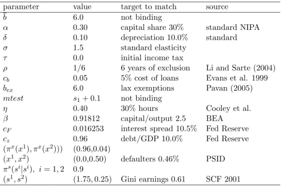
Table 1. Calibration
parameter value target to match source
b 6.0 not binding
α 0.30 capital share 30% standard NIPA
δ 0.10 depreciation 10.0% standard
σ 1.5 standard elasticity
τ 0.0 initial income tax
ρ 1/6 6 years of exclusion Li and Sarte (2004)
cb 0.05 5% cost of loans Evans et al. 1999
bex 6.0 lax exemptions Pavan (2005)
mtest s1+ 0.1 not binding
η 0.40 30% hours Cooley et al.
β 0.91812 capital/output 2.5 BEA
cF 0.016253 interest spread 10.5% Fed Reserve
cz 0.96 debt/GDP 10.0% Fed Reserve
(πx(x1), πx(x2))) (0.96,0.04)
(x1, x2) (0.0,0.50) defaulters 0.46% PSID
πs(si|si), i= 1,2 0.9
(s1, s2) (1.75,0.25) Gini earnings 0.61 SCF 2001
This calibration implies the values for endogenous variables reported in Table 2. The default rate on outstanding debt here is 3.47 per cent, somehow lower than the 4-4.5 per cent charge-off and delinquency rates on credit cards but in line with the figures for all consumer (unsecured) loans reported by the Federal Reserve. The proportion of agents with positive debt is approximately 16 per cent.
Table 2. Benchmark model variable value credit limit −b(s) 0.60 default debt −b(s2, x2) 0.1283 transfers rate tr 0.00 spread λ 0.1050 interest rate r 0.0250 capital stock K 1.4275 labour supply N 0.4087 wage rate w 1.0187 aver. hours 0.2999 Gini earnings 0.6075 debt/GDP 0.1046 default rate 0.03467 proportion defaulting 0.00476 proportion in debt 0.1660
Regarding the credit limit, this is a situation where b= b(s2, x1) > b(s1, x2) and the
con-ditions in Proposition 3(b) are satisfied withb(s2, x2) = −0.1283. Hence b=b(s2, x1) and
the defaulters are agents with low labour productivitys2, high liabilityx2, and assets below b(s2, x2) = −0.1283. The level of debt at which consumption would necessarily have to
become negative is about -0.31. Therefore in this economy there is default in a range of debt b ∈[−0.31,−0.1283] where it would still be feasible for agents not to default, and it involves about 22 per cent of the bankruptcy filings. The rest of filers with assets below -.31 have no other option, however notice that ending up in this position is the result of deliberate forward looking borrowing past choices.
The following Table 3 displays some moments of the distribution. Approximately 3.8 per cent of individuals are clean but hit the borrowing constrain set by banks. There are more low-productivity individuals in this group. There is just under 2 per cent of individuals who are bankrupt and are saving zero. Again a large majority of them have a low productivity.
Table 3. Distribution moments (%) Shock Type Borrowing constrained Total mass
s x Φ(b, s, x,0) Φ(0, s, x,1) Φ(b, s, x,0) Φ(b, s, x,1) s1 x1 0.364 0.186 47.177 0.823 s2 x1 3.273 1.672 46.079 1.921 s1 x2 0.015 0.008 1.966 0.034 s2 x2 0.136 0.070 1.920 0.080 Totals 3.789 1.935 97.142 2.859
For some extra insight, Figure 3 reproduces the policy functionsb0(b, s, x, z) when produc-tivity is lows=s2 and the bankruptcy record is cleanz= 0 for the two realizations of the
liability shock x or ’luck’. The initial flat region at zero on the ‘bad-luck’ curve indicates default. The initial flat region at the level of the constraint b on the ‘normal-luck’ curve indicates borrowing-constrained states.
-1 -0.5 0 0.5 1 1.5 2 2.5 3 3.5 4 -0.6 -0.5 9 -0.5 68 -0.5 35 -0.4 91 -0.4 34 -0.3 66 -0.2 87 -0.1 96 -0.0 93 0.02 18 0.14 79 0.28 57 0.43 52 0.59 63 0.76 9 0.95 34 1.14 95 1.35 72 1.57 65 1.80 75 2.05 01 2.30 44 2.57 03 2.84 78 3.13 7 3.43 79 3.75 04 4.07 45
LOW-PRODUCTIVITY POLICY FUNCTIONS
BAD LUCK
LEVEL OF ASSETS NORMAL LUCK
Fig 3. Policy functions
It remains to verify that this equilibrium survives under price competition. Consider now condition (7). Solving the corresponding off-equilibrium individual problem and distribu-tion, it turns out that (7) holds. The calculations displayed in Table 4 demonstrate this. Propositions 4 therefore implies that there are no profitable feasible credit-line deviations.
Table 4. Off equilibrium deviations (%)
λ? LHS of (10) λ?−cb 1+r+λ?−c b Ld(b,λ?) L(b,λ?) cF 0.105 0.0000 0.050926 0.034673 0.016253 0.090 -0.0134 0.037559 0.034670 0.016253 0.060 -0.0413 0.009662 0.034680 0.016253
5
Policies and welfare
This section reports the consequences of various policy changes on the stationary equilib-rium. I will consider first a more stricter income means test for declaring bankruptcy. It is characterized by a reduction in the value of the parametermtest. This type of shift can be associated with one of the most salient modifications introduced recently in Chapter 7 of the U.S. bankruptcy code.16 The second exercise will consider an increase in the period that an individual remains excluded from credit after a bankruptcy filing. This will be represented by a reduction in the probability of regaining access to the credit marketρ. The result will help assess the importance of the way credit histories are recorded and then used by lenders. For each experiment, I will report and discuss the response of the various endogenous variables displayed in Table 2 and, additionally, some measure of welfare. Welfare W is calculated as the expected value function over asset levels b, productivity s, liability shock
x, and credit status z according to the following W ≡R
Sv(b, s, x, z)dΦ. This is a measure
16The new U.S. Bankruptcy Act came into effect on October 2005. An individual qualifies to declare
of ex-ante welfare. The proportional change inW in equivalent consumption units relative to the corresponding benchmarkWB will be calculated as ∆W C ≡(W/WB)1/(η(1−σ))−1.
5.1 Means testing
In the model, an agent can file for bankruptcy only if her normalised earnings s(1−l) is lower than the value of the means-test parameter mtest. Since only low-productivity (i.e., low s) agents default this parameter begins to have an effect on individual behaviour only when it becomes sufficiently small. In the benchmark the value is so large as to be of no consequence. Now in order to study the response to a tighter bankruptcy rule I will consider a stricter means test which requires that filers have earnings below the average earnings of the bottom half of the distribution. This motivates using mtest = 0.04 in this experi-ment.17 This is an approximation to the kind of median-income test introduced in the new bankruptcy code.18 This value exceeds a defaulter’s earnings in the benchmark equilibrium and is therefore bound to have consequences for the economy.19 Note that meeting the test depends on the leisure choice.
Table 5. Means testing(mtest= 0.04)
variable benchmark endog. BC exog. BC
credit limit −b 0.60 0.65 0.60
default debt −b(s2, x2) 0.1283 0.2093 0.1626
spread λ 0.1050 0.1033 0.1044
deposit interest rate r 0.0250 0.0249 0.0249 lending interest rate r+λ 0.1300 0.1282 0.1293
default rate % 3.467 3.320 3.414 percentage defaulting 0.476 0.4168 0.4567 percentage bankrupt 2.859 2.500 2.740 debt/GDP 0.1046 0.1099 0.1054 capital stock K 1.4275 1.4293 1.4280 labour supply N 0.4087 0.4088 0.4086 wage rate w 1.0187 1.0190 1.0189 aver. hours 0.2999 0.2996 0.2993 %∆W C — -0.246 -0.031
Table 5 shows outcomes for an endogenous borrowing constraint as well as for an exogenous borrowing constraint. With endogenous borrowing limits the decline in welfare is sizeable,
17
The 50% bottom distribution consists of the low-productivity agents withs= 0.25. The average hours
supply within this group is 0.1548. Then the chosen means test corresponds to the average earnings within this group 0.0375.
18
Although a crude one indeed al least for the following two reasons. First, the actual US test refers to average income earned over the previous six months. The model however has not been set up to deal with history dependent rules. Second, the median-income yardstick should be endogenous but here for simplicity I assume it to be exogenously fixed.
19
Supply of hours 1−lis 0.36 and her earnings is thuss2×0.36 = 0.09. If instead of two groups we were
to divide the distribution of earnings more finely, then the median earnings is 0.145, the highest (1−l)s
corresponding to the lowestlof 0.42 among those individuals with lows=s2= 0.25. A test based on this
equivalent to near 0.25 per cent of consumption. With exogenous borrowing limits the change in welfare is negligible instead. Macroeconomic factors (prices) hardly change in either case.
I will analyse the case of endogenous credit limit first. In this case the borrowing con-straint b is part of the endogenous variables. Table 5 shows that the tighter means test leads to a visibly looser credit limit. This is accounted for by the fact that the critical low-productivity/low-liability individual type has less incentive to go bankrupt as expressed by the increase in her default threshold level of debt −b(s2, x1) which determines the credit
limitb. Similarly the low-productivity/high-liability households default from a higher level of debt, −b(s2, x2), too. The explanation is that the means test imposes an extra cost to
declaring bankruptcy since it requires an agent to reduce her labour supply and earnings well below the level that would otherwise be optimal. The aggregate supplies of inputs hardly vary and therefore the deposit interest rate and wage rate remain practically un-changed. There is only a small reduction in the lending interest rate which is reflective of the lower default rate and proportion of bankrupt agents in the economy.
In order to interpret the response of aggregate welfare, the underlying changes in utility levels and the wealth distribution must be examined in some detail. Results are reported for the changes between the benchmark equilibrium and the equilibrium corresponding to the stricter means test mtest= 0.04 with endogenous credit limit. Figure 4 displays the value function for non-bankrupt individuals, i.e. with z = 0, for all the four productivity and liability states and over level of assets.20 The utility at most individual states is only slightly
lower with the means test. It only declines markedly for the low-productivity/high-liability (s2, x2) individuals with high debts in the default region where the value function becomes
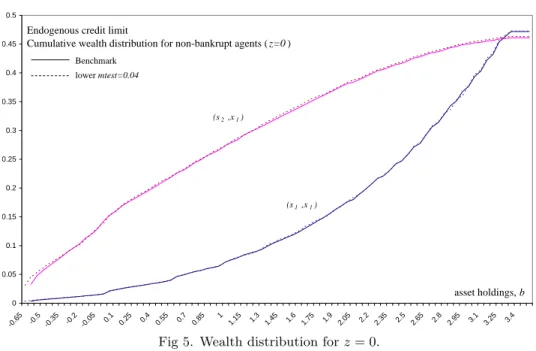
flat. Also note that the looser credit limit expands the lower domain of the value func-tion. Turning now to the wealth distribution, Figure 5 depicts the cumulative distribution of non-bankrupt low-liability agents over asset levels.21 Overall there is little change with only a visible rise in the mass of low-productivity agents at high levels of debt. All in all, the aggregate decline in welfare follows from changes in both the value function and distri-bution for low-productivity agents with high levels of debt in or near the bankruptcy region. The downward shift in the value function must be caused by the response of prices and the borrowing constraint, and the direct cost of the means test. Since the general equilibrium changes in prices can be ignored, one can focus on the credit limit and the means test. The means test forces defaulting individuals to sacrifice leisure and income in the filing period. Bankruptcy then becomes less attractive as an option to share risks. The looser credit limit allows agents to borrow more and, in particular, the low-income/high-liability individual will do so before using the default option by reducingb(s2, x2). This lowers the reservation
utility where bankruptcy takes places and thus the utility of agents in the default state. On the other hand, the rise in the mass of the distribution at high levels of debt reflects the shift of agents towards higher debt positions as a consequence of the looser borrowing constraint. This increase in the number of non-bankrupt agents must match the reduction in the proportion of bankrupt individuals reported in Table 5.
20
The figures in this section are constructed on an evenly spaced grid. However, the computations are performed on an unevenly spaced and less dense grid. This accounts for the apparent lack of smoothness in the curves represented.
-45 -43 -41 -39 -37 -35 -33 -31 -0.6 5 -0.5 5 -0.4 5 -0.3 5 -0.2 5 -0.1 5 -0.0 5 0.050.150.250.350.450.550.650.750.850.951.051.151.251.351.451.551.651.751.851.952.052.152.252.352.452.552.652.752.852.95
Endogenous credit limit
Value function for non-bankrupt agents (z=0)
asset holdings, b Benchmark lower mtest=0.04 (s2 ,x2) (s2 ,x1) (s1 ,x2) (s1 ,x1)
Fig 4. Value function forz= 0.
0 0.05 0.1 0.15 0.2 0.25 0.3 0.35 0.4 0.45 0.5 -0.6 5 -0.5 -0.35 -0.2 -0.05 0.1 0.25 0.4 0.55 0.7 0.85 1 1.15 1.3 1.45 1.6 1.75 1.9 2.05 2.2 2.35 2.5 2.65 2.8 2.95 3.1 3.25 3.4
Endogenous credit limit
Cumulative wealth distribution for non-bankrupt agents (z=0)
Benchmark lower mtest=0.04
asset holdings, b
(s1 ,x1)
(s2 ,x1)
Fig 5. Wealth distribution forz= 0.
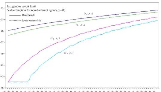
Consider now the means-test experiment when the credit limit is held constant at its bench-mark level. Except for the constant credit limit, the other variables change in the same direction as with the endogenous credit limit. The scale of the changes is much milder though, including the decline in welfare. Figures 6 and 7 depict the value function and wealth distribution for non-bankrupt agents. The value function declines only slightly in the default states and the distribution shows no noticeable change.
-45 -43 -41 -39 -37 -35 -33 -31 -0.6 5 -0.5 5 -0.4 5 -0.3 5 -0.2 5 -0.1 5 -0.0 5 0.050.150.250.350.450.550.650.750.850.951.051.151.251.351.451.551.651.751.851.952.052.152.252.352.452.552.652.752.852.95
Exogenous credit limit
Value function for non-bankrupt agents (z=0)
Benchmark lower mtest=0.04 (s1 ,x1) (s1 ,x2) (s2 ,x1) (s2 ,x2)
Fig 6. Value function forz= 0.
0 0.05 0.1 0.15 0.2 0.25 0.3 0.35 0.4 0.45 0.5 -0.6 5 -0.5 -0.35 -0.2 -0.05 0.1 0.25 0.4 0.55 0.7 0.85 1 1.15 1.3 1.45 1.6 1.75 1.9 2.05 2.2 2.35 2.5 2.65 2.8 2.95 3.1 3.25 3.4
Exogenous credit limit
Cumulative wealth distribution for non-bankrupt agents (z=0)
Benchmark lower mtest=0.04
(s2 ,x1)
(s1 ,x1)
Fig 7. Wealth distribution forz= 0.
Summing up, when the credit limit is endogenous much of the welfare consequences of a means test are driven by the implications of the subsequent loosening of the credit limit. Welfare declines because of the adverse effect on utility levels among defaulters and the shift in the distribution towards high debt individuals. With exogenous credit limit the effect on the utility levels is much milder and there is no change in the distribution. Does this depend on the design of the experiment? A stricter means test, includingmtestof 0.02 and 0.0, also implies a much larger decline with endogenous credit limits through the same mechanism.22 In either case the effect of this policy change on the general economy is fairly negligible since the aggregate incidence of default responds very little. Agents can and do adjust their labour supply in order to meet the means test and still declare bankruptcy. For this reason this exercise might be missing important aspects of a tighter bankruptcy code.
22
The exercise withmtest= 0.02 implies a reduction in welfare of -0.376 with an endogenous credit limit
5.2 Punishment period
In this model, an individual who files for bankruptcy will be excluded from credit for a period with average length 1/ρ, whereρ is the probability of regaining a good credit score. The experiment in this section increases the exclusion period from six to twelve years.
Table 6. Punishment period (1/ρ= 12)
variable benchmark endog. BC exog. BC
credit limit −b 0.60 0.77 0.60
default debt −b(s2, x2) 0.1283 0.3214 0.2273
spread λ 0.1050 0.1009 0.1023
deposit interest rate r 0.0250 0.0253 0.0242 lending interest rate r+λ 0.1300 0.1262 0.1265
default rate % 3.467 3.104 3.2342 debt/GDP 0.1046 0.1200 0.0960 percentage defaulting 0.476 0.3498 0.3661 percentage bankrupt 2.859 4.196 4.391 capital stock K 1.4275 1.4255 1.4420 labour supply N 0.4087 0.4094 0.4089 wage rate w 1.0187 1.0178 1.0216 aver. hours 0.2999 0.3016 0.3004 %∆W C — -2.979 -2.256
Table 6 shows outcomes for an endogenous borrowing constraint as well as for an exogenous borrowing constraint. In the two cases, the decline in welfare following the harsher pun-ishment is sizeable, equivalent to near 3 per cent of consumption with endogenous credit limits, and 2.25 per cent with fixed credit limits. With endogenous borrowing limits the decline in welfare is thus more pronounced. Macroeconomic factors (prices) change mildly in different directions in the two cases. The lending rate declines by about the same amount though regardless.
I will analyse the case where the borrowing constraint is endogenous first. Table 6 shows that the longer bankruptcy flag leads to a much looser credit limit −b since the critical low-productivity/low-liability individual is less inclined to go bankrupt. That is, her de-fault level of debt −b(s2, x1) is higher. This is also true for the default threshold of the
low-productivy/high-liability individual −b(s2, x2). The reason is that a longer ban from
borrowing limits risk sharing for a bankrupt individual and therefore raises their cost of bankruptcy. This results in the lower default rate but, on the other hand, an appreciably larger proportion of agents locked in the bankruptcy state. The aggregate supplies of inputs change only slightly. The negligible increase in the deposit interest rate combined with the decrease in the default risk lead to a modest reduction in the lending interest rate of about 4 basis points.
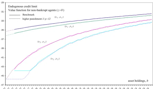
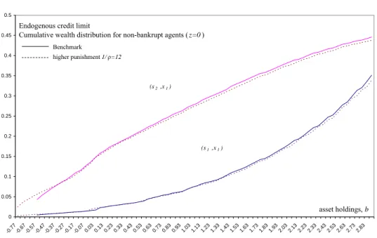
In order to understand the response of welfare, consider again the background changes in the value function and the wealth distribution for non-bankrupt agents. Figure 8 displays the value functions for both the benchmark calibration and the longer exclusion punishment. The utility level at most individual states remains practically unchanged or is only negligibly lower with the harsher punishment. Utility declines markedly for the