Monetary Policy Transmission and House Prices:
European Cross-country Evidence
K
AI
C
ARSTENSEN
O
LIVER
H
ÜLSEWIG
T
IMO
W
OLLMERSHÄUSER
CES
IFO
W
ORKING
P
APER
N
O
.
2750
CATEGORY 7: MONETARY POLICY AND INTERNATIONAL FINANCE
AUGUST 2009
An electronic version of the paper may be downloaded
• from the SSRN website: www.SSRN.com
• from the RePEc website: www.RePEc.org
CESifo Working Paper No. 2750
Monetary Policy Transmission and House Prices:
European Cross-country Evidence
Abstract
This paper explores the importance of housing and mortgage market heterogeneity in 12 European countries for the transmission of monetary policy. We use a panel VAR model which is estimated over the period 1995–2006 to generate impulse responses of key macroeconomic variables to a monetary policy shock. We propose a data–driven approach that splits our panel of countries into two disjoint groups according to the impact of the monetary policy shock on real house prices. Our results show that in countries with a more pronounced reaction of real house prices the propagation of monetary policy shocks to macroeconomic variables is amplified.
JEL Code: C32, C33, E52.
Keywords: panel VAR model, house prices, monetary policy transmission, country clusters, sign restrictions.
Kai Carstensen
Ifo Institute for Economic Research at the University of Munich
Poschingerstrasse 5 Germany - 81679 Munich
carstensen@ifo.de
Oliver Hülsewig
Ifo Institute for Economic Research at the University of Munich
Poschingerstrasse 5 Germany - 81679 Munich
huelsewig@ifo.de Timo Wollmershäuser
Ifo Institute for Economic Research at the University of Munich
Poschingerstrasse 5 Germany - 81679 Munich
wollmershaeuser@ifo.de
July 30, 2009
We thank Anindya Banerjee, Monika Piazzesi, Carlo Rosa, Stephanie Schmitt–Grohé, Jiri Slacalek, Jan–Egbert Sturm, Martín Uribe and Frank Westermann for helpful comments and suggestions, and Johannes Mayr and Steffen Elstner for helping us with collecting the data. We also thank Christophe André from the OECD’s Economics Department for kindly providing us with the house price data. The usual disclaimer applies. The research leading to these results has received funding from the European Community’s Seventh Framework
1
Introduction
The role of the housing market for the transmission of monetary policy has attracted great attention in the last few years, both empirically and theoretically (see, e.g., Mishkin, 2007, and Muellbauer and Murphy, 2008). Empirically, the recent business cycle experience indicates that house price fluctuations can have tremendous macroeconomic consequences. Theoretically, the calibrated dynamic stochastic general equilibrium (DSGE) models by Iacoviello (2005), Iacoviello and Neri (2007), Monacelli (2009), and Pari`es and Notarpietro (2008) suggest that credit market frictions in the form of housing collateral constraints can amplify the effects of monetary policy shocks on the macroeconomy in a quantitatively relevant magnitude. These models also imply that the extent to which the housing market affects the propagation of monetary policy is related to the institutional characteristics of mortgage markets and therefore different between heterogeneous countries.
This paper empirically explores the role of housing for the transmission of monetary policy in a panel of 12 European countries. In particular, we analyze whether there are cross–country differences in the response of house prices to a monetary policy shock and how these differences relate to the reaction of other important macroeconomic variables. Indeed we find that countries exhibiting a strong response of house prices also show a strong reaction of output, consump-tion and inflaconsump-tion. We interpret this result as evidence for the importance of the housing market for the transmission of monetary policy. We also show that the magnitude of the house price reaction across countries is correlated with standard measures of mortgage market flexibility. However, this correlation is far from perfect which suggests that other cross–country features, such as the share of the housing sector in overall economic activity, regulations regarding housing taxes and subsidies or transaction costs, are also likely to be relevant.
These results are derived by estimating panel vector autoregressive (VAR) models from which we calculate impulse responses of key macroeconomic vari-ables to a monetary policy shock. The panel dimension allows us to concentrate on the short time period from 1995 Q1 to 2006 Q4. We select this period since the process of deregulation of mortgage markets has been accomplished mostly
until the mid–1990s (Girouard and Bl¨ondal, 2001), even though certain restric-tions still exist. Moreover, the disinflationary process had been completed in most European countries in the mid–1990s and monetary regimes had become very similar across countries, both of which is essential in the context of evalu-ating the effects of a monetary policy shock in a cross–country study.
Notwithstanding the deepening of the European economic integration, sev-eral institutional characteristics of mortgage markets still continue to differ be-tween countries. In order to detect heterogeneities in the transmission of a structural shock in the context of a panel VAR model we suggest a novel data– driven approach that clusters countries into disjoint groups according to the impact a monetary policy shock has on real house prices. We split our panel of countries into two groups – a strong reaction group and a weak reaction group – that are endogenously identified by using a distance measure, which is de-termined by the absolute difference between the cumulated impulse responses of real house prices to a standardized monetary policy shock. This stands in contrast to the standard procedure to preselect countries into different groups according to some specific housing market indicators that are a priori chosen without knowing their relation to the monetary transmission process.
So far, a number of papers have adressed the role the housing market plays in the propagation of monetary policy shocks. Mishkin (2007) and Muellbauer and Murphy (2008) highlight the most important transmission channels. On the one hand, house prices are affected by, inter alia, the housing stock, credit availability and ultimately changes in interest rates induced by monetary policy (Muellbauer and Murphy, 2008). On the other hand, house price fluctuations have an impact on consumption decisions of households – via housing wealth and housing collateral effects – and residential investment – e.g. via Tobin’s q by affecting the value of housing relative to construction costs (Goodhart and Hofmann, 2008).
To quantitatively explore the reaction of house prices to a monetary pol-icy shock, many papers have employed single–country VAR models. Iacoviello (2002), Iacoviello and Minetti (2003), Giuliodori (2005), IMF (2008) and Calza, Monacelli, and Stracca (2006) find that house prices across European countries respond differently to changes in interest rates. The differences in the reaction
of house prices are shown to be related to country–specific characteristics of national mortgage markets. Countries where mortgage markets are more devel-oped experience a higher volatility of house prices and a greater role for housing in the transmission of monetary policy. However, a quantitative comparison of the effects is difficult to establish because the estimates reported are often imprecise due to low degrees of freedom.
Goodhart and Hofmann (2008) suggest using a panel VAR model to increase the power and the efficiency of the analysis. They assess the link between real output, monetary variables and house prices for a panel of 17 OECD countries over the period from 1973 to 2006. They find a significant relationship between these variables, which has become stronger in the period from 1985 to 2006 af-ter mortgage markets have been liberalized substantially. Assenmacher-Wesche and Gerlach (2008) also estimate a panel VAR model for the same set of OECD countries over the period from 1986 to 2006. In order to assess the role of insti-tutional characteristics of mortgage markets for the transmission of monetary policy, they split their panel of countries into different groups. The sub–panels are exogenously determined by using a broad range of indicators that reflect cross–country differences in the structure of mortgage financing. They conclude that institutional characteristics of mortgage markets across countries shape the response of house prices to monetary policy shocks, but the differences between the groups are quantitatively unessential.
Overall, the evidence suggests that housing in European countries plays a role in the transmission of monetary policy, but it is difficult to identify the cross-country differences precisely. While the development of mortgage markets is likely a source of heterogeneity, the separation of countries by means of in-stitutional indicators is cumbersome since (i) a general agreement on which of the indicators are most important is missing, (ii) the classification of the indi-cators is often arbitrary, and (iii) indiindi-cators for a particular country often have an opposite impact on the transmission of monetary impulses. Our data–driven approach of forming country clusters avoids these shortcomings. The results suggest that heterogeneity of housing and mortgage markets across countries reflects differences in the transmission of monetary policy, which can be ex-plained by the amplifying effects that arise from movements in real house prices
after a monetary policy shock. Since the discrepancies are sizable, we conclude that monetary policy should be concerned about the influence of house prices when setting interest rates.
The remainder of the paper is organized as follows. In Section 2, the VAR model for a single panel of countries is presented. We generate impulse re-sponses to a monetary policy shock to explore the reaction of real house prices to an innovation in interest rates. Section 3 sets out our approach of identi-fying disjoint groups of countries. We discuss the institutional characteristics of mortgage markets across countries, describe our data–driven methodology of clustering countries and comment our findings. In Section 4, we compare im-pulse responses of the identified groups of countries to a monetary policy shock to assess the influence of movements in real house prices. Section 5 discusses the plausibility of our results against the background of a calibrated DSGE model. Section 6 provides concluding remarks.
2
A Single Panel VAR Model
Consider a panel VAR model in reduced form:
Xi,t =ci+ p
X
j=1
AjXi,t−j +εi,t, (1)
where Xi,t is a vector of endogenous variables for country i, ci is a vector of
country-specific intercepts, Aj is a matrix of autoregressive coefficients for lag
j, p is the number of lags and εi,t is a vector of error terms. The vector Xi,t
consists of four variables
Xi,t = [yi,t pi,t si,t hpi,t]′, (2)
whereyi,t denotes real GDP,pi,t is the overall price level, measured by the GDP
deflator, si,t is the nominal short–term interest rate, which serves as the policy
instrument of the central banks and hpi,t are real house prices – i.e. nominal
house prices deflated with the GDP deflator. For each variable, we use a pooled set of M · T observations, where M denotes the number of countries and T
The VAR model is estimated via Bayesian methods using quarterly data for 12 European countries that are mainly taken from the OECD covering the period from 1995Q1 to 2006Q4.1
Our panel of countries comprises Belgium (BEL), Denmark (DNK), Finland (FIN), France (FRA), Germany (GER), Ire-land (IRL), Italy (ITA), the NetherIre-lands (NED), Portugal (PRT), Spain (ESP), Sweden (SWE) and the United Kingdom (GBR). All variables are in logs – ex-cept for the nominal short–term interest rate, which is expressed in percent – and linearly de–trended. The matrix of constant terms c comprises individual country dummies that account for possible heterogeneity across the units. We use a lag order of p= 3, which ensures that the residuals are free of first–order serial correlation as indicated by the LM test of Baltagi (2005, pp. 97).2
Based on the VAR model (1) we generate impulse responses of the variables to a monetary policy shock. As in Canova and de Nicolo (2002), Peersman (2005) and Uhlig (2005) we identify the shock by imposing sign restrictions that incorporate the notion that a contractionary monetary policy shock has a non–positive impact on real output (yt), the overall price level (pt) and real
house prices (hpt) as well as a non–negative impact on the short–term interest
rate (st). While the restrictions imposed on real output, the price level and the
short–term interest rate are standard (Peersman, 2005), the restriction imposed on real house prices follows from theoretical considerations derived from DSGE models which incorporate a housing sector and which show that real house prices should decline on impact after a monetary contraction rather than rise.3
For all variables the time period over which the sign restrictions are binding is set equal to two quarters. The restrictions are imposed as ≤or ≥.4
1
Appendix A provides a detailed description of the data. Since mortgage markets in European countries experienced an extensive phase of liberalization (IMF, 2008), which started in the early 1980s and ended in the mid 1990s (Girouard and Bl¨ondal, 2001), we decided to focus on the period after the process of deregulation has been accomplished.
2
See Appendix B for the results of tests for first–order serial correlation. 3
See for example the papers by Iacoviello (2005), Iacoviello and Neri (2007), Monacelli (2009), and Pari`es and Notarpietro (2008)
4
The advantage of sign restrictions over Cholesky or Blanchard–Quah decompositions is that we do not have to impose zero restrictions on the contemporaneous or long–run im-pact of shocks. Short-run restrictions are typically inconsistent with a large class of general equilibrium models (Canova and Pina, 2005), and long-run restrictions may be substantially
Figure 1: Single Panel VAR Model: Impulse Responses to a Monetary Policy Shock 0 4 8 12 16 −5 −4 −3 −2 −1 0 0 4 8 12 16 −5 −4 −3 −2 −1 0 Real output 0 4 8 12 16 −5 −4 −3 −2 −1 0 0 4 8 12 16 −3 −2 −1 0 0 4 8 12 16 −3 −2 −1 0
Overall price level
0 4 8 12 16 −3 −2 −1 0 0 4 8 12 16 0 1 2 0 4 8 12 16 0 1 2 Interest rate 0 4 8 12 16 0 1 2 0 4 8 12 16 −15 −10 −5 0 0 4 8 12 16 −15 −10 −5 0
Real house prices
0 4 8 12 16
−15 −10 −5 0
Notes: The solid lines denote the median of the impulse responses, which are identified from a Bayesian vector–autoregression with 1000 draws using sign restrictions. The shaded areas are the related 68% confidence intervals. Real output, the overall price level and real house prices are expressed in percent terms, while the interest rate is expressed in units of percentage points at an annual rate.
Figure 1 shows the impulse responses of the variables to a contractionary monetary policy shock, which is normalized to unity, i.e. 100 basis points.5
The solid lines display the median of the impulse responses and the shaded areas are the 68% confidence intervals. As the median and the quantiles were com-puted from all impulse responses that satisfy the sign restrictions, the confidence intervals not only reflect sampling uncertainty, but also modeling uncertainty stemming from the non–uniqueness of the identified monetary policy shock. The simulation horizon, which is depicted on the horizontal axis, covers 20 quarters. The responses of real output, the overall price level and real house prices are expressed in percent terms, while the response of the interest rate is expressed in units of percentage points at an annual rate. Notice that the immediate responses of all variables are constrained after the impact so that little interpre-tation needs to be given to the sign of the adjustment for the first two quarters. Real output falls after the monetary policy shock and remains below the baseline value for around 20 quarters. The decline in the overall price level is very persistent. The short–term interest rate remains above baseline for around 8 quarters. Real house prices display a hump–shaped response – which is consis-tent with the findings of e.g. Assenmacher-Wesche and Gerlach (2008), Iacoviello and Minetti (2003) and Calza, Monacelli, and Stracca (2006) – and return grad-ually to the baseline value after around 20 quarters. Considering the responses of the overall price level and real house prices two remarks are in order. First, nominal house prices – calculated as real house prices plus the overall price level – decline in reaction to a contractionary monetary policy shock. Second, the adjustment of nominal house prices is more flexible than the adjustment of the overall price level over the simulation horizon.
biased in small samples (Faust and Leeper, 1997). The sign restrictions approach only makes explicit use of restrictions that we often use implicitly. Having a certain theoretical un-derstanding in mind, researchers using the Cholesky or the Blanchard–Quah decomposition typically experiment with the model specification until the impulse responses look reasonable (Peersman, 2005). This a priori theorizing is made more explicit with sign restrictions.
5
The Bayesian estimation and the identification of the monetary policy shock us-ing sign restrictions were performed with Fabio Canova’s MATLAB codes bvar.m,
bvar chol impulse.m and bvar sign ident.m, which can be downloaded from his website (http://www.crei.cat/people/canova/).
We check the robustness of our results by generating impulse responses of the variables to a monetary policy shock, which is identified by imposing a Cholesky–decomposition of the variance–covariance matrix of the reduced–form shocks (see Appendix C). While the signs of the responses are identical to those obtained under the sign restrictions approach (at least after two quarters), the effects of a monetary policy shock are less pronounced and more delayed and the confidence bands are tighter when the Cholesky–decomposition is applied.
3
Identification of Cross–country
Heterogene-ity
So far, we have estimated the panel VAR model (1) by assuming that systematic cross–country differences can be explained exclusively by country–specific inter-cepts. If, however, the country–specific institutional characteristics of housing and mortgage markets largely differ, also the dynamic adjustment in response to structural shocks is likely be heterogenous across countries. Interpreting the reaction of real house prices to a monetary policy shock as a general func-tion of the country–specific housing and mortgage market characteristics, the VAR parameters should depend on these characteristics and, hence, the impulse responses should differ from country to country. Therefore, countrywise estima-tion would be optimal. Unfortunately, the precise estimaestima-tion of impulse response coefficients within the VAR framework requires a relatively large number of ob-servations. Since for the reasons outlined above a reasonable sample does not start before 1995, we need to construct country panels in order to increase the number of observations by using the cross–section dimension. Before presenting our procedure of splitting a panel of countries into disjoint sub–panels, the fol-lowing Section gives an overview of the institutional characteristics of mortgage markets across European countries.
3.1
Institutional Heterogeneity of Mortgage Markets
As emphasized by Maclennan, Muellbauer, and Stephens (1998) the institu-tional characteristics of mortgage markets across European countries constitute
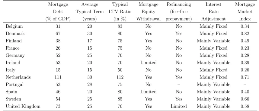
a source of heterogeneity for the role of housing in the transmission of monetary policy. Some key characteristics are summarized in Table 1, which depicts a number of institutional indicators that potentially have a bearing on the sen-sitivity of house prices to a change in interest rates (Calza, Monacelli, and Stracca, 2006).
Heterogeneity in the depth of mortgage markets across European countries is reflected by the volume of mortgage credit relative to GDP, which varies considerably. In the Netherlands, the United Kingdom and Denmark the ratios are relatively high, ranging between 111% and 67%, while Italy, France and Belgium report the lowest ratios.
The access of households to mortgage credit depends on several factors (IMF, 2008), such as the standard length of mortgage loan contracts, the typical loan–to–value (LTV) ratio, the ability of mortgage equity withdrawals and the capability to prepay mortgages without fees. Longer mortgage debt contracts keep the ratio between debt services and income affordable. High LTV ratios allow households to take out more debt, while the ability to borrow against ac-cumulated home equity allows households to tap their housing wealth directly. The possibility of early repayment enables households to refinance their mort-gage debt in the event of an interest rate decline. Finally, the composition of mortgages between variable–rate and fixed–rate is also potentially important (Tsatsaronis and Zhu, 2004). Mortgage debt contracts designed with variable mortgage rates lower the debt burden of households when short–term interest rates decline, but at the expense of a higher burden when short–term interest rates rise.
The IMF (2008) distinguishes the development of mortgage markets across countries by means of a synthetic mortgage market index to exploit the diver-sity in explaining the role of housing for the transmission of monetary policy.6
The index is constructed as a simple average of several institutional indicators
6
Our discussion on the separation of countries refers mainly to the results of the IMF (2008), but we are aware of a number of studies – see Giuliodori (2005), Tsatsaronis and Zhu (2004) and Calza, Monacelli, and Stracca (2006), among others – that proceed along similar lines. These studies classify countries into homogenous groups taking account of several institutional indicators. Compared to the results of the IMF (2008), the outcome is akin.
and lies between 0 and 1, yielding that higher values reflect a high degree of development, while lower values indicate that the development is minor.7
According to the IMF (2008), mortgage markets in Denmark, Sweden and the Netherlands appear most developed, which suggests a high potential role for housing in the transmission of monetary policy. In these countries the standard length of mortgage debt contracts is around 30 years, the typical LTV ratios are about 80% and mortgage products specifically designed for equity withdrawals are widely marketed. In contrast mortgage markets in France, Germany and Italy appear less developed, as the typical LTV ratios ranges only between 50% to 75% and the ability of mortgage equity withdrawals is widely missing.
However, the distinction of countries by means of institutional indicators is disputable (Assenmacher-Wesche and Gerlach, 2008). First, the selection of the indicators is subjective. Vagueness prevails in the decision on which of the indi-cators is relevant. Second, the indiindi-cators are compiled arbitrarily. For instance a considerable degree of judgement is required – see ECB (2003) – to decide on the relevant LTV ratios (using the average ratio or the maximum ratio), to as-sess whether restrictions on early repayment fees are implemented or to evaluate whether mortgage rates are variable or fixed because both terms often coexist. Third, indicators for a particular country often have an opposite impact on the transmission of monetary impulses. While in Belgium, for example, the typical LTV ratio is above average, suggesting a relatively strong impact of interest rate changes on GDP, the prevalence of fixed–rate debt contracts or the impossibility of borrowing against home equity for consumption rather attenuate the trans-mission of monetary policy shocks. Since the classification of countries on the basis of institutional indicators suffers from these shortcomings, we propose an alternative approach, which lets the data decide whether housing and mortgage market heterogeneity is relevant for monetary policy transmission.
7
Table 1: Institutional Characteristics of Mortgage Markets
Mortgage Average Typical Mortgage Refinancing Interest Mortgage Debt Typical Term LTV Ratio Equity (fee–free Rate Market (% of GDP) (years) (in %) Withdrawal prepayment) Adjustment Index
Belgium 31 20 83 No No Mainly Fixed 0.34
Denmark 67 30 80 Yes Yes Mainly Fixed 0.82
Finland 38 17 75 Yes No Mainly Variable 0.49
France 26 15 75 No No Mainly Fixed 0.23
Germany 52 25 70 No No Mainly Fixed 0.28
Ireland 53 20 70 Limited No Mainly Variable 0.39
Italy 15 15 50 No No Mainly Fixed 0.26
Netherlands 111 30 112 Yes Yes Mainly Fixed 0.71
Portugal 53 28 75 No – Mainly Variable –
Spain 46 20 80 Limited No Mainly Variable 0.40
Sweden 54 25 85 Yes Yes Mainly Variable 0.66
United Kingdom 73 25 70 Yes Limited Mainly Variable 0.58
Sources: IMF (2008), Calza, Monacelli, and Stracca (2006) and Tsatsaronis and Zhu (2004).
3.2
Data–driven Identification of Cross–country
Hetero-geneity
Instead of dividing our panel of countries a priori according to the country– specific institutional characteristics, we split our panel into disjoint sub–groups by focusing on the response of real house prices to a monetary policy shock. To facilitate an easy distinction between such country panels, we consider only two of them, namely a strong reaction groupand a weak reaction group.
3.2.1 Methodology
The allocation of the countries of our panel to one of these two groups is achieved in three steps.
1. Step: Define and Estimate the Distance between Sup–panels To
quantify the difference between any two sub–panels of countries, we need to define a distance measure. As we are interested in the different impulse responses of real house prices after a monetary policy shock, we use
d= q X k=1 b α1k− q X i=1 b α2k , (3)
where αb1k and αb2k are the median responses of real house prices of the first
and second sub–panel, respectively, k periods after the occurrence of the shock. We consider the responses of up to q lags. Hence, the distance measure d in expression (3) reflects the absolute value of the difference between the cumulated impulse responses over the first q quarters.
At first sight, it is now straightforward to allocate each country to either the
strong reaction group or the weak reaction group. One can simply estimate all possible pairs of sub–panels and choose the pair with the largest distance. This approach resembles a cluster algorithm, where the number of clusters is fixed and the distance between the cluster centers (i.e., the impulse response coefficients) is maximized. However, we have to bear in mind that the impulse response coefficients are not observed but estimated. Hence, choosing the maximum distance pair only would contaminate the choice by a considerable portion of
randomness. In fact, we find that there a many different pairs of sub–panels that exhibit similar distance measures.
2. Step: Select Pairs of Sub–panels with Significant Distance Measure
Therefore, we proceed as follows. We estimate panel VAR models for all possible pairs of sub–panels, which contain at least three countries to ensure enough de-grees of freedom for each sub–panel.8
Overall the number of pairs of sub–panels amounts to 1969.9
For all pairs of sub–panels we generate impulse responses to a monetary policy shock, which is identified by imposing sign restrictions, and calculate the distance measure.
Then, we identify all pairs of sub–panels that exhibit a significant distance measure, where significance is detected as follows. Assume that the estimated impulse response coefficients αb1k andαb2k asymptotically follow a normal
distri-bution. Then the sums of the coefficients considered for the distance measure, denoted by bs1 =
Pq
k=1αb1k and bs2 =
Pq
k=1αb2k, are also asymptotically normal.
Under the null hypothesis that all pairs of sub–panels are identical and have the same sum of population coefficientss=Pqk=1αi, the only systematic difference
in the estimation results is the size of the panel from which they are estimated. The sums of the estimated coefficients should be approximately distributed as: b s1−s ∼ N 0, σ 2 /(N1T) (4) b s2−s ∼ N 0, σ 2 /(N2T) , (5)
where N1 is the size of the first sub–panel, N2 is the size of the second sub–
panel, T is the number of observations corrected for the number of lags pin the VAR model and σ2
is the population variance that is assumed to be constant across countries. Furthermore, assuming that the countries are independent, we
8
As before, the VAR models contain the same set of variables – real output, the overall price level, the short–term interest rate and real house prices – and a lag length of p= 3.
9
Notice that in our panel the total number of disjoint pairs of sub–panels amounts to 2048 (= 212
/2). Given that we consider only pairs of sub–panels containing at least three countries, this reduces the number of pairs to 1969, since there is one combination without any country, 12 combinations with only one country and 66 combinations – (11×12)/2 – with two countries.
can apply a classical two–sided difference test using the statistic: d = bs1−bs2.
Under the null hypothesis, the statistic is approximately normally distributed with mean zero and variance:
Var(d) =σ2 /(N1T) +σ 2 /(N2T) = (1/N1+ 1/N2)σ 2 /T. (6) Since σ2
is unknown, we estimate the population variance from expression (6) by noting that:
σ2
=TVar(d)/(1/N1+ 1/N2), (7)
where the sample variance of the distance measure Var(d) is calculated from the numerous realizations of d. Given the estimate ofσ2
, we construct a t–statistic and compare it with the corresponding 95% critical value of the t–distribution. As a result, we have identified all those pairs of sub–panels that are signif-icantly different from each other. If there was no significant difference at all, we would conclude that all countries show the same house price response to a monetary policy shock and terminate the analysis here. However, we find 831 (634) significant distance measures, if we set q= 4 (q= 8). In contrast to using only the maximum–distance pair, we thus consider all the different ways to split the panel of countries into significantly different sub–panels. Thereby, we alle-viate the problem that the impulse response coefficients, and hence the distance measure, are subject to estimation uncertainty. However, this approach in turn raises the question how to allocate a single country to either the strong reaction group or the weak reaction group.
3. Step: Allocate each Country to either the Strong or the Weak Reaction Group The allocation problem is tackled in the final step. Using the pairs of sub–panels with a significant distance measure we calculate the frequency that a specific country belongs to the sub–panels with the stronger reaction of real house prices to a monetary policy shock. If this frequency is above a threshold that is determined below, then the respective country is allocated to the strong reaction group, otherwise it is allocated to the weak reaction group.
The idea behind this rule is as follows. Assume there are three “true” strong reaction countries. Then we should expect that the distance measure is
maxi-mized when these three countries are put into one sub–panel and all the others in the other sub–panel. However, due to sampling error, a different pair of sub– panels may actually exhibit the largest distance. Using our approach, we may at least expect to find each of the three strong reaction countries to be more often in the strong reaction sub–panel than any of the other countries.
To accomplish this, we derive a threshold for the frequency that a specific country belongs to the strong reaction sub–panels. From the previous step we know which pairs of sub–panels are significantly different from each other. Now we count how many times each country is in a strong reaction sub–panel. A priorily, each country has the same chance to be a strong reaction country. Hence, under this null hypothesis there is, for each pair of sub–panels, a 50% chance that a specific country is in the strong reaction sub–panel. Now assume that there are a total of Nc different pairs of sub–panels of which n exhibit a
significant distance measure. Then, for each country, the number of times it is in the strong reaction sub–panel resembles a random experiment, wheren draws without replacement are taken from a population of size Nc that is composed
of 50% white (=strong reaction) and 50% black (=weak reaction) elements. Accordingly, the frequency x – that a particular country is found to be in the
strong reaction group – follows a hypergeometric distribution: f(x;Nc, Nc/2, n),
where the number of pairs Nc depends on the total number of countriesM and
the minimum size of a sub–panel.10
Finally, from the hypergeometric distribution we derive a 95% critical value for the frequency that a particular country belongs to thestrong reaction group. If any country is selected more often, it is unlikely that this is due to pure chance. Hence, we allocate these countries to the strong reaction group. All other countries are allocated to the weak reaction group.
10
Let us denote the the minimum size of a sub–panel by m. Then the number of pos-sible pairs of sub–panels can be calculated as Nc =
PM−m l=m
M l
!
. In our case, with
M = 12 countries and a minimum sub–panel size of m = 3, we have Nc = 3938 pairs. Of
these pairs, we have to estimate only 3938/2 = 1969 because, e.g., the ordering of the pair
A ={1,2,3,4,5,6}, B ={7,8,9,10,11,12} or A ={7,8,9,10,11,12}, B ={1,2,3,4,5,6} is irrelevant, whileex ante either AorB could be the strong reaction sub–panel.
3.2.2 Identified Country Groups
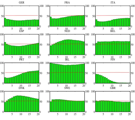
The separation of countries according to the above steps leads to two disjoint sub–panels that depart in the reaction of real house prices to a monetary policy shock. Figure 2 plots the relative frequency of belonging to the strong reac-tion group – as measured by means of the cumulative impulse responses of real house prices over the first q quarters – together with the critical value of the hypergeometric distribution.
For most of the countries in our sample the classification is independent from the value ofq. Countries like Germany, Italy and Finland are clearly identified as belonging to theweak reaction group, whereas countries like Belgium and Ireland are allocated to the strong reaction groupfor all values of q. For the subsequent analysis we set q = 4, which corresponds to the quarter in which real house prices reach their trough following the monetary policy shock. However, Figure 2 shows the allocation of countries is robust against variations of q between 3 and 8 quarters. The classification of countries yields that Belgium, Denmark, Ireland, the Netherlands, Sweden and the United Kingdom are settled in the
strong reaction group, as in these countries the reaction of real house prices to a monetary policy shock is significantly more pronounced. In contrast Finland, France, Germany, Italy, Portugal and Spain belong to the weak reaction group
because their relative frequency is below the critical value.11
This classification is also robust against the choice of the critical value of the two–sided difference test applied in the second step of the allocation algorithm. Given our assumption that the estimated impulse response coefficients asymp-totically follow a normal distribution, we tested the significance of the distance measure by calculating at–statistic and comparing it with the 95% critical value of a t–distribution (which is equal to 1.8125 with N1+N2−2 = 10 degrees of
freedom). However, as the small sample validity of the asymptotics is problem-atic, it is not clear whether the distance measure really follows a t–distribution.
11
Forq= 4 our approach leads to the following ranking of countries as measured by the re-spective relative frequency: Ireland (94.12%), Denmark (64.59%), Belgium (63.99%), Sweden (60.50%), the Netherlands (57.86%), the United Kingdom (54.74%), Spain (46.10%), Finland (37.70%), France (37.45%), Germany (31.81%), Portugal (27.61%) and Italy (22.81%). Notice that the 95% critical value of belonging to thestrong reaction groupis 52.58%.
Figure 2: Frequency of Belonging to the Strong Reaction Group 5 10 15 20 0 50 100 GER 0 50 100 5 10 15 20 0 50 100 FRA 0 50 100 5 10 15 20 0 50 100 ITA 0 50 100 5 10 15 20 0 50 100 ESP 0 50 100 5 10 15 20 0 50 100 NED 0 50 100 5 10 15 20 0 50 100 BEL 0 50 100 5 10 15 20 0 50 100 PRT 0 50 100 5 10 15 20 0 50 100 IRL 0 50 100 5 10 15 20 0 50 100 FIN 0 50 100 5 10 15 20 0 50 100 DNK 0 50 100 5 10 15 20 0 50 100 SWE 0 50 100 5 10 15 20 0 50 100 GBR 0 50 100
Notes: The bars show the frequency of belonging to thestrong reaction groupin percent. The quartersqover which the impulse responses of real house prices are accumulated, are depicted on the horizontal axis. Out of the total of 1969 pairs of sub–panels, the number of disjoint sub–panelsn, which show a significant distance measure, falls from 1165 forq= 1 to 655 for
q= 20. The horizontal line shows the critical value of the hypergeometric distribution, which slightly increases from 52.02% for q = 1 to 52.98% for q = 20. If the frequency is greater or equal than the critical value, the frequency with which a country appears in the strong reaction groupis significant.
To see if our classification depends on the choice of the critical value, we re–ran the three–step allocation algorithm using a 90% critical value of at–distribution (which is equal to 1.3722) and a 99% critical value of a t–distribution (which is equal to 2.7638). Figure 9 in Appendix D shows that if the true critical value of the unknown distribution lies somewhere between these two critical values of the t–distribution, the allocation of the countries to the two groups remains unchanged for values of q= 3 to 8.
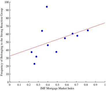
Even though our classification of countries is roughly in line with the mort-gage market index of the IMF (2008), some important differences are in order (see Figure 3). First, the rankings of countries are different. We obtain for Ire-land the highest relative frequency, followed by Denmark, Belgium and Sweden, while the mortgage market index assigns Denmark the highest value, followed by the Netherlands and Sweden. Second, the composition differs. We find that Ireland and Belgium are settled in the strong reaction group, although both countries obtain relatively low values in the mortgage market index.
We interpret our findings as an indication that the development of mortgage markets across countries is important in shaping the reaction of house prices to a monetary policy shock, but additional country–specific characteristics, such as national traditions, cultural factors, the share of the housing sector in overall economic activity, the number of employees in the construction sector, regula-tions regarding housing taxes and subsidies or transaction costs might also be relevant (see for example ECB, 2003).
4
Results
What are the macroeconomic consequences of mortgage market heterogeneity across countries? To address this question we re–estimate a panel VAR model for the strong reaction group and the weak reaction group separately and compare the responses of the variables to a monetary policy shock, which is identified by imposing sign restrictions.12
Figure 4 reports the impulse responses of the variables in both groups together with the confidence regions of the responses
12
Figure 3: Comparison with IMF Mortgage Market Index 0 0.1 0.2 0.3 0.4 0.5 0.6 0.7 0.8 0.9 1 0 10 20 30 40 50 60 70 80 90 100
IMF Mortgage Market Index
Frequency of Belonging to the Strong Reaction Group
Notes: The vertical axis depicts the relative frequency of belonging to the strong reaction groupas measured by means of the cumulative impulse responses of real house prices over the first q = 4 quarters. For the IMF Mortgage Market Index see also Table 1. Note that the IMF does not calculate the index for Portugal.
resulting from the estimation of the weak reaction group, which are marked by the shaded areas. While some of the median impulse responses of the two sub– panels are statistically not different (in particular the initial response of the overall price level), the differences are quantitatively significant in any case.
In both sub–panels real output falls after the monetary policy shock, but the decline in the strong reaction group is more than twice as large on impact (−3.5% versus −1.5%) and remains significantly more pronounced over the en-tire simulation horizon. The fall of prices in the strong reaction group is also larger on impact (−2% versus −1%) and the price level remains significantly below that of the weak reaction group. The reaction of the short–term interest rate to a monetary policy shock is almost identical for both sub–panels, which ensures that the differences in the responses of the remaining variables in the VAR models are not due to a different evolution of the short–term nominal
terest rate.13
The reaction of real house prices in both sub–panels also differs substantially and significantly as the drop in the strong reaction group is two times larger on impact (−6% versus−3%) and still three times larger after four quarters (−15% versus−5%) when the house price response reaches its trough. The findings exhibit that the adjustment of the variables in both groups of countries depart – to some extent even substantially – after a monetary policy shock. The heterogeneity across countries seems to reflect the differences in the transmission of monetary policy, which can be related to the amplifying influence of house prices in propagating monetary policy shocks. We interpret the discrepancy in the adjustment as sizable enough to conclude that monetary policy should be concerned about movements in real house prices when setting interest rates.
In order to get a deeper insight in the way the monetary policy shock is transmitted to the macroeconomy, we estimate an extended panel VAR model for both sub–panels, which includes an additional variable that potentially plays a role for the propagation mechanism. The vector of endogenous variables for country i is given by:
Xi,t = [yi,t pi,t si,t hpi,t zi,t]′, (8)
where (zi,t) is the additional variable of interest, which is either given by real
private consumption, real residential investment or the mortgage rate. The variables summarized by (zi,t) are expressed in logs – except for the mortgage
rate that is in percent – and linearly detrended.
The inclusion of private consumption by households follows from the idea that spending plans are likely affected by movements in house prices due to housing wealth and housing collateral effects (Muellbauer and Murphy, 2008). Households may increase their consumption expenditures in response to an in-crease in housing wealth induced by a shift of house prices.14
Additionally,
13
As before the monetary policy shock is normalized to unity, i.e. 100 basis points. 14
It is, however, important to note that an increase in housing wealth is different from a rise in financial wealth. As housing fulfills a dual role, serving as both a real asset and a commodity yielding service, an increase in the value of housing assets causes a redistribution of wealth within the household sector. Therefore the impact on consumption expenditure arising through wealth effects should be limited (Muellbauer and Murphy, 2008).
Figure 4: Impulse responses of country groups 0 4 8 12 16 −4 −3 −2 −1 0 1 0 4 8 12 16 −4 −3 −2 −1 0 1 Real output 0 4 8 12 16 −4 −3 −2 −1 0 1 strong weak 0 4 8 12 16 −3 −2 −1 0 0 4 8 12 16 −3 −2 −1 0
Overall price level
0 4 8 12 16 −3 −2 −1 0 strong weak 0 4 8 12 16 0 1 2 0 4 8 12 16 0 1 2 Interest rate 0 4 8 12 16 0 1 2 strong weak 0 4 8 12 16 −15 −10 −5 0 0 4 8 12 16 −15 −10 −5 0
Real house prices
0 4 8 12 16 −15 −10 −5 0 strong weak
Notes: The solid (dashed) lines denote the median of the impulse responses of the strong (weak) reaction group. The shaded areas refer to the 68% confidence intervals resulting from the estimation of theweak reaction group. All impulse response functions are identified from a Bayesian vector–autoregression with 1000 draws using sign restrictions. Real output, the overall price level and real house prices are expressed in percent terms, while the interest rate is expressed in units of percentage points at an annual rate.
households may rise their consumption expenditures because of an easier access to credit, since an increase in house prices extends the value of collateral, which loosens credit constraints. The strength of both effects depends – inter alia – on the sensitivity of house prices to a change in interest rates. Residential invest-ment may be stimulated by an increase in house prices, primarily because the value of housing rises relative to construction costs. Finally, including the mort-gage rate accounts for the speed with which debt contracts conditions adapt to a change in interest rates.
We assess heterogeneity across the two sub–panels by focusing on the reaction of the additional variables to a monetary policy shock.15
The impulse responses are plotted in Figure 5, together with the confidence regions of the responses resulting from the estimation of the weak reaction group, which are marked by the shaded areas.
Figure 5: Extended VAR Model Specifications
0 4 8 12 16 −4 −2 0 0 4 8 12 16 −4 −2 0 Private consumption 0 4 8 12 16 −4 −2 0 strong weak 0 4 8 12 16 −15 −10 −5 0 0 4 8 12 16 −15 −10 −5 0 Residential investment 0 4 8 12 16 −15 −10 −5 0 strong weak 0 4 8 12 16 0 1 2 0 4 8 12 16 0 1 2 Mortgage rate 0 4 8 12 16 0 1 2 strong weak
Notes: The solid (dashed) lines denote the median of the impulse responses of the strong (weak) reaction group. The shaded areas refer to the 68% confidence intervals resulting from the estimation of theweak reaction group. All impulse response functions are identified from a Bayesian vector–autoregression with 1000 draws using sign restrictions. Private consumption and residential investment are expressed in percent terms, while the mortgage rate is expressed in units of percentage points at an annual rate.
15
In line with the four–variable VAR model we impose a non–positive reaction on private consumption and residential investment and a non–negative reaction on mortgage rates over the first two quarters following the monetary policy shock.
The findings exhibit that real private consumption in both sub–panels re-sponds differently to a monetary policy shock, as the fall in the strong reaction group is significantly more pronounced. This suggests that the reaction of pri-vate consumption is affected by the volatility of real house prices due to wealth and collateral effects. The response of real residential investment in both sub– panels seems to be alike, except for the reaction in the first year following the shock, where the reduction is larger in the strong reaction group than in the
weak reaction group.
Mortgages rates in both sub–panels move differently. While in thestrong re-action groupmortgage rates overshoot the increase in short–term interest rates, the adjustment in the weak reaction group is only incomplete and more persis-tent, indicating a slower pass–through of changed refinancing costs to mortgage rates. While this discrepancy in the adjustment of mortgage rates might be attributable to diverging debt contract terms, it turns out, however, that in the two sub–panels both, variable–rate and fixed–rate contracts, co–exist (see Table 1).
5
Plausibility of the Estimated Effects of
Hous-ing Market Heterogeneity
The extent to which the real economy is affected by a monetary policy shock does not only depend on the degree of financial frictions. Non–neutrality of monetary policy is possibly also related to other sources of rigidities, such as the stickiness of prices and wages or adjustment costs on the markets for labor and investment goods. An empirical impulse response analysis is hardly able to distinguish between these different sources and to draw clear inference about the true structural reasons behind the differences in the response of macroeconomic variables to a monetary policy shock. Even though we have shown that real output co–moves with real house prices following a monetary policy shock and that there exists a positive correlation between the amplitude of the two impulse response functions, heterogeneity in the extent of other rigidities may also play a certain role in shaping the cross–country difference of the impulse responses.
Therefore, we evaluate the plausibility of our estimated effects of housing market heterogeneity by comparing the empirical impulse responses with im-pulse responses obtained from a calibrated New Keynesian DSGE model that incorporates a housing sector. We refer to the model of Iacoviello (2005), which includes two frictions that render monetary policy non–neutral: a borrowing constraint (`a la Kiyotaki and Moore, 1997) on the part of entrepreneurs, who produce an intermediate good in a competitive market by using real estate and labor as inputs, and nominal price stickiness (`a la Calvo, 1983) on the part of the retailers, who produce a differentiated final good under monopolistic com-petition using the intermediate good as an input.
Our exercise proceeds in two steps. In a first step, we quantify the effects of mortgage market heterogeneity by simulating the model with two LTV ratios, 50% (which corresponds to the lowest ratio in our panel of countries, see Table 1) and 100% (which is still below the highest ratio in our panel of countries), and a fixed probability of not changing prices (θ = 0.75).16
We are particularly interested in the differences between the impulse responses of real output and real house prices to a monetary policy shock. In a second step, we perform the same exercise with a fixed LTV ratio (89%) and different degrees of price stickiness. Based on evidence from surveys among firms, ´Alvarez (2008) reports that the mean duration of price changes in our panel of countries varies between 8.2 months in the United Kingdom (implying θ = 0.63) and 13.5 months in Germany (implying θ = 0.77).17
Figure 6 summarizes the results by showing the differences of the theoretical impulse responses to a monetary policy shock. Two conclusions can be drawn from the calibration exercise. First, the higher the LTV ratio (i.e. the less the entrepreneurs are credit constrained), the larger the immediate effects of an unexpected 1% monetary policy contraction on real house prices and real output. The effects are sizeable and are of comparable
16
Except for the LTV ratio the calibration is identical with Iacoviello (2005). The impulse responses were computed using the “basic” model of Iacoviello (2005). In contrast to the “full” model, financial frictions only apply to entrepreneurs, and the use of capital is excluded from the production process. Moreover, in order to isolate the mechanism of the financial accelerator, the central bank is assumed to not respond to movements in output.
17
Notice that in the work of ´Alvarez (2008) comparable information on price stickiness in Ireland, Denmark and Finland is missing.
Figure 6: Evidence from a DSGE Model 0 4 8 12 16 −2 −1.5 −1 −0.5 0 0.5
Real output differential
0 4 8 12 16 −2 −1.5 −1 −0.5 0 0.5
Real house price differential
(LTV=100%) minus (LTV=50%) (θ=0.77) minus (θ=0.63)
Notes: The solid (dashed–dotted) lines show the difference between the impulse responses to a contractionary 1% monetary policy shock obtained from the basic Iacoviello (2005) model with a strong financial accelerator mechanism (a high degree degree of price stickiness θ) and those obtained from the same model with a weak financial accelerator mechanism (a low degree degree of price stickiness θ). The values on the vertical axis are units of percentage points.
magnitude to our empirical results, at least in the first quarters following the shock. In case of a LTV ratio of 100% real output declines by 1.5 percentage points more than in case of a LTV ratio of 50%. Likewise the drop in real house prices is much more pronounced in case of a stronger financial accelerator. Thus, heterogeneity in the characteristics of mortgage markets are likely to have a substantial impact on the real effects of monetary policy. Second, the stickier prices are, the larger is the immediate effect of an unexpected 1% monetary policy contraction on real house prices and real output. In case of a high degree of price stickiness real output and real house prices decline by 0.4 percentage points more on impact than in case of a low degree of price stickiness. Thus, differences in the degree of price stickiness are also likely to be a source of divergences in the transmission of monetary policy.
Since both frictions have similar implications for the cross–country differ-ences of monetary policy effects, an empirical impulse–response analysis alone is unable to discriminate between the sources of these differences, irrespective
Figure 7: Effects of Monetary Policy on Real House Prices and Price Stickiness 5 6 7 8 9 10 11 12 13 14 15 0 10 20 30 40 50 60 70 80 90 100
Mean Duration of Price Changes
Frequency of Belonging to the Strong Reaction Group
Notes: The vertical axis depicts the relative frequency of belonging to the strong reaction groupas measured by means of the cumulative impulse responses of real house prices over the firstq= 4 quarters. The horizontal axis shows the mean duration of price changes in months, which is taken from ´Alvarez (2008). Note that data for Ireland, Denmark and Finland is missing.
of whether real house prices are included in the VAR model or not. In order to rule out that different degrees of price stickiness drive our results, we plotted the relative frequency of belonging to the strong reaction group against the mean duration of price changes (see Figure 7). The negative relationship implies that in countries with a strong real house price and real output response to a mone-tary policy shock prices are more flexible than in the countries belonging to the
weak reaction group. If anything, then cross–country differences in the degree of price stickiness should attenuate the differences between the impulse responses in the two country groups, rather than being their source.
6
Concluding Remarks
We explore the role of housing market heterogeneity in European countries for the transmission of monetary policy. We estimate a panel VAR model to gen-erate impulse responses of key macroeconomic variables to a monetary policy shock taking special account of the reaction of real house prices. Our panel comprises 12 countries for which we use quarterly data over the period from 1995 to 2006.
We find that key macroeconomic variables in European countries co–move with real house prices after a monetary policy shock. In order to assess the impact of housing and mortgage market heterogeneity across countries we split our panel into two disjoint groups – a strong reaction group and a weak reac-tion group – using a data–driven approach that takes account of the reaction of real house prices to a monetary policy shock. This is in contrast to the ex-isting literature – notably to Assenmacher-Wesche and Gerlach (2008) – which typically splits the panel a priori using a broad range of indicators that reflect cross–country differences in the structure of housing and mortgage markets.
A comparison of the impulse responses of the two groups yields that quan-titatively significant differences exist. The reaction of macroeconomic variables in the strong reaction group (including Ireland, Sweden, the Netherlands, Den-mark, Belgium and the United Kingdom) is more pronounced than in the weak reaction group(including Finland, France, Germany, Italy, Spain and Portugal), which suggests that real house prices play an amplifying role in the propagation of monetary policy shocks. Our result stands in contrast to Assenmacher-Wesche and Gerlach (2008) who find that institutional characteristics of mortgage mar-kets across countries shape the response of house prices to monetary policy shocks, but the differences between the groups are quantitatively unessential. As regards the discrepancies of the responses of major macroeconomic variables after a monetary policy shock across our groups of countries, we conclude that monetary policy should take account of the volatility of real house prices when setting interest rates.
References
´
Alvarez, L. J.(2008): “What Do Micro Price Data Tell Us on the Validity of the New Keynesian Phillips Curve?,” Economics - The Access, Open-Assessment E-Journal, 2(19).
Assenmacher-Wesche, K., and S. Gerlach (2008): “Ensuring Financial
Stability: Financial Structure and the Impact of Monetary Policy on Asset Prices,” CEPR Discussion Paper 6773, Centre for Economic Policy Research.
Baltagi, B. H. (2005): Econometric Analysis of Panel Data. John Wiley & Sons, Chichester, 3rd edn.
Bjørnland, H. C., and D. H. Jacobsen (2008): “The role of house prices
in the monetary policy transmission mechanism in the U.S,” Working Paper 2008/24, Norges Bank.
Calvo, G. A.(1983): “Staggered Prices in a Utility–Maximizing Framework,”
Journal of Monetary Economics, 12, 383–398.
Calza, A., T. Monacelli, and L. Stracca (2006): “Mortgage Markets,
Collateral Constraints, and Monetary Policy: Do Institutional Factors Mat-ter?,” CEPR Discussion Paper 6231, Centre for Economic Policy Research.
Canova, F., and G. de Nicolo (2002): “Monetary Disturbances Matter
for Business Fluctuations in the G-7,” Journal of Monetary Economics, 49, 1131–1159.
Canova, F., and J. Pina (2005): “What VAR Tell us about DSGE Models,”
in New Trends in Macroeconomics, ed. by C. Diebolt, and C. Kyrtsou, pp. 89–124. Springer.
ECB (2003): “Structural Factors in the EU Housin Markets,” Structural issues report, European Central Bank.
Faust, J., and E. Leeper (1997): “When Do Long Run Identifying
Restric-tions Give Reliable Results?,” Journal of Business and Economic Statistics, 15(3), 345–353.
Girouard, N., and S. Bl¨ondal (2001): “House Prices and Economic Activ-ity,” OECD Economics Department Working Papers 279, OECD Economics Department.
Giuliodori, M.(2005): “Monetary Policy Shocks and the Role of House Prices across European Countires,” Scottish Journal of Political Economy, 52, 519– 543.
Goodhart, C., and B. Hofmann(2008): “House Prices, Money, Credit, and
the Macroeconomy,”Oxford Review of Economic Policy, 24, 180–205.
Iacoviello, M. (2002): “House Prices and the Business Cycles in Europe: A
VAR Analysis,” Boston College Working Papers in Economics 540, Boston College Department of Economics.
(2005): “House Prices, Borrowing Constraints, and Monetary Policy in the Business Cycle,” American Economic Review, 95, 739–764.
Iacoviello, M., and R. Minetti (2003): “Financial Liberalisation and the
Sensitivity of House Prices to Monetary Policy: Theory and Evidence,” The Manchester School, 71, 20–34.
Iacoviello, M., and S. Neri (2007): “Housing Market Spillovers: Evidence
from an Estimated DSGE Model,” Boston College Working Papers in Eco-nomics 659, Boston College Department of EcoEco-nomics.
IMF (2008): World Economic Outlook April 2008. International Monetary Fund, New York.
Kiyotaki, N., and J. Moore (1997): “Credit Cycles,” Journal of Political
Economy, 105(2), 211–48.
Maclennan, D., J. Muellbauer, andM. Stephens(1998): “Asymmetries
in Housing and Financial Market Institutions and EMU,” Oxford Review of Economic Policy, 14, 54–80.
Mishkin, F. S.(2007): “Housing and the Monetary Transmission Mechanism,” Finance and Economics Discussion Series 2007-40, Board of Governors of the Federal Reserve System (U.S.).
Monacelli, T. (2009): “New Keynesian Models, Durable Goods, and
Collat-eral Constraints,” Journal of Monetary Economics, forthcoming.
Muellbauer, J., and A. Murphy (2008): “Housing Markets and the
Econ-omy: The Assessment,” Oxford Review of Economic Policy, 24, 1–33.
Pari`es, M. D., and A. Notarpietro(2008): “Monetary Policy and Housing
Prices in an Estimated DSGE Model for the US and the Euro Area,” Working Paper Series 972, European Central Bank.
Peersman, G. (2005): “What Caused the Early Millennium Slowdown?
Ev-idence Based on Vector Autoregressions,” Journal of Applied Econometrics, 20, 185–207.
Sims, C. A. (1980): “Macroeconomics and Reality,” Econometrica, 48, 1–48.
Tsatsaronis, K., and H. Zhu (2004): “What drives House Price Dynamics:
Cross–Country Evidence,” BIS Quarterly Review, March, 65–79.
Uhlig, H. (2005): “What are the Effects of Monetary Policy on Output?
Re-sults from an Agnostic Identifcation Procedure,” Journal of Monetary Eco-nomics, 52, 381–419.
Appendices
A
Data
We use data for 12 European countries that is mainly taken from the OECD covering the period from 1995Q1 to 2006Q4. The panel of countries includes Belgium, Denmark, Finland, France, Germany, Ireland, Italy, the Netherlands, Portugal, Spain, Sweden and the United Kingdom. The data refers to the OECD Economic Outlook Nr. 84 database and comprises:
1. Real output (yt): Gross domestic product, volume, market prices,
season-ally adjusted.
2. Overall price level (pt): Gross domestic product, deflator, market prices,
seasonally adjusted.
3. Interest rate (st): Short-term interest rate in percent.
4. Real house prices (hpt): Nominal house prices provided by the OECD,
de-flated with the GDP deflator, seasonally adjusted. Nominal house prices for Belgium and Portugal are taken from the Bank of International Set-tlement (BIS) database.
5. Private consumption: Private final consumption expenditure, volume, sea-sonally adjusted.
6. Residential investment: Private residential fixed capital formation, vol-ume, seasonally adjusted. Since residential investment is not available for Portugal we used the gross fixed capital formation, volume, seasonally adjusted, instead.
7. Mortgage rate: National mortgage rates are taken from the European Central Bank (www.ecb.org).
B
Tests for Serial Correlation
Following Baltagi (2005), we adopt an LM test for first-order serial correlation. The results of the tests, which are summarized in Table 2, show that the model appears to be well specified.
Table 2: Univariate LM Tests for Serial Correlation Variable Test statistic p–value
εy 0.021 0.89
εp 0.004 0.95
εs 0.220 0.64
εhp 0.695 0.40
Notes: Results of an LM Test for first-order serial correlation. See Baltagi (2005, pp. 97).
C
Single Panel VAR Model: Alternative Identification
Scheme
We check the robustness of our results by generating impulse responses of the variables to a monetary policy shock, which is identified by imposing a Cholesky– decomposition of the variance–covariance matrix of the reduced–form shocks (Sims, 1980). The ordering of variables in the vector Xi,t implies that real
output and the overall price level are hit by an innovation in the nominal short– term interest rate with a lag of one quarter, while real house prices are affected contemporaneously. The impulse responses of the variables are shown in Figure 8 together with the corresponding error bounds.
The findings show that real output falls after two quarters following a mon-etary policy shock, exhibiting a humped–shaped response, and returns to the baseline value subsequently. Prices fall immediately. Real house prices slightly increase on impact after a monetary policy shock, but the rise is statistically insignificant. They decline afterwards, reaching their trough after around 8 quarters, and return to the baseline value subsequently.
While the identification strategy seems to be irrelevant for the response of the short–term nominal interest rate, a comparison of the remaining impulse
Figure 8: Alternative Identification Scheme 0 4 8 12 16 −1 −0.5 0 0 4 8 12 16 −1 −0.5 0 Real output 0 4 8 12 16 −1 −0.5 0 0 4 8 12 16 −0.5 −0.4 −0.3 −0.2 −0.1 0 0 4 8 12 16 −0.5 −0.4 −0.3 −0.2 −0.1 0
Overall price level
0 4 8 12 16 −0.5 −0.4 −0.3 −0.2 −0.1 0 0 4 8 12 16 0 0.5 1 1.5 0 4 8 12 16 0 0.5 1 1.5 Interest rate 0 4 8 12 16 0 0.5 1 1.5 0 4 8 12 16 −2 −1 0 1 0 4 8 12 16 −2 −1 0 1
Real house prices
0 4 8 12 16
−2 −1 0 1
Notes: The solid lines denote the median of the impulse responses, which are identified from a Bayesian vector–autoregression with 1000 draws using a triangular decomposition of the variance–covariance matrix of the reduced–form shocks. The shaded areas are the related 68% confidence intervals. Real output, the overall price level and real house prices are expressed in percent terms, while the interest rate is expressed in units of percentage points at an annual rate.
responses with those resulting from the sign restriction approach yields some important differences. Using the triangular decomposition the effects of a mon-etary policy shock are less pronounced and more delayed (see Peersman, 2005, and Bjørnland and Jacobsen, 2008, for similar results). Under sign restrictions an unexpected 100 basis point increase in the policy instrument depresses real output instantaneously by almost 3%, whereas the triangular decomposition leads to a decline in real output by slightly less than 1% after two years. The maximum impact on the overall price level using the triangular decomposition is
−0.3% in the third year following the shock, compared to −2.0% in the second year under sign restrictions. Likewise, the fall in real house prices is about seven times larger under sign restrictions.
Moreover, the confidence bands are tighter when the triangular decomposi-tion is applied. Since the triangular decomposidecomposi-tion is unique, there is no un-certainty stemming from the identification of the monetary policy shock. Thus, the confidence intervals exclusively reflect sampling uncertainty, which is re-lated to the Bayesian estimation of the coefficients of the reduced–form VAR model. Under the sign restriction approach the uncertainty surrounding the impulse response functions increases due to the existence of multiple orthogonal decompositions of the variance–covariance matrix, which satisfy the imposed sign restrictions.
D
Robustness of the Allocation Algorithm
Figure 9: Frequency of Belonging to the Strong Reaction Group
5 10 15 20 0 50 100 GER 0 50 100 5 10 15 20 0 50 100 FRA 0 50 100 5 10 15 20 0 50 100 ITA 0 50 100 5 10 15 20 0 50 100 ESP 0 50 100 5 10 15 20 0 50 100 NED 0 50 100 5 10 15 20 0 50 100 BEL 0 50 100 5 10 15 20 0 50 100 PRT 0 50 100 5 10 15 20 0 50 100 IRL 0 50 100 5 10 15 20 0 50 100 FIN 0 50 100 5 10 15 20 0 50 100 DNK 0 50 100 5 10 15 20 0 50 100 SWE 0 50 100 5 10 15 20 0 50 100 GBR 0 50 100 5 10 15 20 0 50 100 GER 0 50 100 5 10 15 20 0 50 100 FRA 0 50 100 5 10 15 20 0 50 100 ITA 0 50 100 5 10 15 20 0 50 100 ESP 0 50 100 5 10 15 20 0 50 100 NED 0 50 100 5 10 15 20 0 50 100 BEL 0 50 100 5 10 15 20 0 50 100 PRT 0 50 100 5 10 15 20 0 50 100 IRL 0 50 100 5 10 15 20 0 50 100 FIN 0 50 100 5 10 15 20 0 50 100 DNK 0 50 100 5 10 15 20 0 50 100 SWE 0 50 100 5 10 15 20 0 50 100 GBR 0 50 100
Notes: The left (right) panel shows the frequencies of belonging to the strong reaction group, if the critical value of the two–sided difference test is equal to 1.3722 (2.7638).
CESifo Working Paper Series
for full list see Twww.cesifo-group.org/wpT
(address: Poschingerstr. 5, 81679 Munich, Germany, office@cesifo.de)
___________________________________________________________________________
2685 Peter Egger, Christian Keuschnigg and Hannes Winner, Incorporation and Taxation:
Theory and Firm-level Evidence, June 2009
2686 Chrysovalantou Milliou and Emmanuel Petrakis, Timing of Technology Adoption and
Product Market Competition, June 2009
2687 Hans Degryse, Frank de Jong and Jérémie Lefebvre, An Empirical Analysis of Legal
Insider Trading in the Netherlands, June 2009
2688 Subhasish M. Chowdhury, Dan Kovenock and Roman M. Sheremeta, An Experimental
Investigation of Colonel Blotto Games, June 2009
2689 Alexander Chudik, M. Hashem Pesaran and Elisa Tosetti, Weak and Strong Cross
Section Dependence and Estimation of Large Panels, June 2009
2690 Mohamed El Hedi Arouri and Christophe Rault, On the Influence of Oil Prices on Stock
Markets: Evidence from Panel Analysis in GCC Countries, June 2009
2691 Lars P. Feld and Christoph A. Schaltegger, Political Stability and Fiscal Policy – Time
Series Evidence for the Swiss Federal Level since 1849, June 2009
2692 Michael Funke and Marc Gronwald, A Convex Hull Approach to Counterfactual
Analysis of Trade Openness and Growth, June 2009
2693 Patricia Funk and Christina Gathmann, Does Direct Democracy Reduce the Size of
Government? New Evidence from Historical Data, 1890-2000, June 2009
2694 Kirsten Wandschneider and Nikolaus Wolf, Shooting on a Moving Target: Explaining
European Bank Rates during the Interwar Period, June 2009
2695 J. Atsu Amegashie, Third-Party Intervention in Conflicts and the Indirect Samaritan’s
Dilemma, June 2009
2696 Enrico Spolaore and Romain Wacziarg, War and Relatedness, June 2009
2697 Steven Brakman, Charles van Marrewijk and Arjen van Witteloostuijn, Market
Liberalization in the European Natural Gas Market – the Importance of Capacity Constraints and Efficiency Differences, July 2009
2698 Huifang Tian, John Whalley and Yuezhou Cai, Trade Sanctions, Financial Transfers
and BRIC’s Participation in Global Climate Change Negotiations, July 2009
2699 Axel Dreher and Justina A. V. Fischer, Government Decentralization as a Disincentive