Numerical Methods for Fluid Structure Interaction, and their Application to Flag Flapping

(1)

Numerical methods for fluid-structure interaction, and

their application to flag flapping

Thesis by

Andres Goza

In Partial Fulfillment of the Requirements for the degree of

Doctor of Philosophy

CALIFORNIA INSTITUTE OF TECHNOLOGY Pasadena, California

2018

(2)

(3)

iii

ACKNOWLEDGEMENTS

I am indebted to many people who over these past several years have informed my view on research, fluid mechanics, mathematics, advising, teaching, squash, movies and storytelling, comedy, and much more. Perhaps most of all, I am grateful that they have made my growth in these areas a journey that I will look back on so fondly. I first thank Tim. Beyond your intimidating instincts for and knowledge of fluid mechanics and applied mathematics, your tireless efforts as an advisor had a huge impact on me. I think what I will remember most are moments you spent teaching me about writing and presenting, discussing advising philosophies, or cracking a witty joke (on the rare occasion that occurred!). I will try my hardest to be as wonderful an advisor as you were to me.

I am also grateful to my committee for being such sources of inspiration and guidance during my time here. John, thank you for your heroic efforts in helping me hone in on the narrative for inverted flag flapping, and for acting as a second advisor to me. Guillaume, thank you for your jokes and willingness to give as good as you get, and for taking the time to meet with me about this thesis and life after graduate school. Mory, your pioneering work on inverted flag flapping is singularly responsible for my pursuit of that topic, and I feel honored to have you on my committee.

I must also thank Aaron, Jomela, Ed, Jay, Chen, Jeeson, Oliver, George, Gianmarco, Sebastian, Vedran, Phillipe, Kazuki, Andre 2.0, Marcus, Ke, and Francisco for making my time in Thomas, Steele, and Gates-Thomas so much more rewarding than it would have been without you. I am particularly grateful to Aaron, whose mathematical intuition was always a source of intimidation and inspiration for me; and to Phillipe for being the best colleague in fluid-structure interaction that I could have asked for.

Thanks also to Paul, Massari, Matt, Alex, and Ron for being such wonderful friends outside of research. I will always remember the nights out on the town, bowling events, softball games, squash matches, and general tomfoolery that your friendships afforded me.

(4)

the whole world throughout both my graduate and undergraduate days. My thanks also go out to Rachel, Matt, Gianmarco, and Marina for being there for me at various times.

Most influential of all have been my family, who believed in me and supported me for longer than I can remember. Mom, Dad, Laurie and Jules, I am only beginning to realize how much effort you have taken to prioritize me and give me every opportunity possible, and I will never forget it.

(5)

v

ABSTRACT

This thesis is divided into two parts. Part I is devoted to the development of numerical techniques for simulating fluid-structure interaction (FSI) systems and for educing important physical mechanisms that drive these systems’ behavior; part II discusses the application of many of these techniques to investigate a specific FSI system.

Within part I, we first describe a procedure for accurately computing the stresses on an immersed surface using the immersed boundary method. This is a key step to simulating FSI problems, as the surface stresses simultaneously dictate the motion of the structure and enforce the no-slip boundary condition on the fluid. At the same time, accurate stress computations are also important for applications involving rigid bodies that are either stationary or moving with prescribed kinematics (e.g., characterizing the performance of wings and aerodynamic bodies in unsteady flows or understanding and controlling flow separation around bluff bodies). Thus, the method is first formulated for the rigid-body prescribed-kinematics case. The pro-cedure described therein is subsequently incorporated into an immersed boundary method for efficiently simulating FSI problems involving arbitrarily large structural motions and rotations.

While these techniques can be used to perform high-fidelity simulations of FSI systems, the resulting data often involves a range of spatial and temporal scales in both the structure and the fluid and are thus typically difficult to interpret directly. The remainder of part I is therefore devoted to extending tools regularly used for understanding complex flows to FSI systems. We focus in particular on the application of global linear stability analysis and snapshot-based data analysis (such as dynamic mode decomposition and proper orthogonal decomposition) to FSI problems. To our knowledge, these techniques had not been applied to deforming-body problems in a manner that that accounts for both the fluid and structure leading up to this work.

(6)

(7)

vii

PUBLISHED CONTENT AND CONTRIBUTIONS

Andres Goza et al. “Accurate computation of surface stresses and forces with immersed boundary methods”. In: Journal of Computational Physics 321 (2016), pp. 860–873. DOI: 10.1016/j.jcp.2016.06.014

AJG established the equation for the surface stresses as a first-kind integral equation, identified the connection between differentiability of the smeared delta functions and the quality of the resulting stresses, ran all simulations, and was the primary author of the article.

Andres Goza and Timothy Colonius. “A strongly-coupled immersed-boundary formulation for thin elastic structures”. In: Journal of Computational Physics336 (2017), pp. 401–411. DOI: 10.1016/j.jcp.2017.02.027

AJG devised and implemented the numerical method, ran all simulations, and was the primary author of the article.

Andres Goza and Timothy Colonius. “A global mode analysis of flapping flags”. In: Turbulence and Shear Flow Phenomena 10. Chicago, Illinois, 2017.

AJG devised and implemented the numerical method, ran all simulations, and was the primary author of the article.

Andres Goza, Timothy Colonius and John E. Sader. “Nonlinear simulations and global modes of inverted flag flapping”. Submitted to theJournal of Fluid Mechan-ics.

AJG identified the mechanism responsible for the onset of flapping, distinguished parameters under which vortex-induced vibration occurs in large-amplitude flap-ping, characterized the chaotic regime, ran all simulations, and was the primary author of the article.

Andres Goza and Timothy Colonius. “Data analysis of fluid-structure interaction”. In preparation.

(8)

I Numerical methods for fluid-structure interaction

1

Chapter I: Introduction . . . 2

Chapter II: Accurately computing surface stresses and forces with immersed boundary methods . . . 4

2.1 Introduction . . . 4

2.2 Demonstrating and resolving inaccurate computation of source terms for a model problem . . . 6

2.3 Extension to accurately computing surface stresses and forces . . . . 15

2.4 An impulsively rotated cylinder . . . 18

2.5 A cylinder in cross-flow . . . 21

2.6 Conclusions . . . 23

Chapter III: An efficient immersed-boundary method for fluid-structure inter-action . . . 25

3.2 Governing equations . . . 26

3.3 Numerical method . . . 28

3.4 Verification on flapping flag problems . . . 34

3.5 An efficient iteration procedure in primitive variables . . . 41

Chapter IV: Global stability analysis of fluid-structure interaction . . . 44

4.2 Numerical method . . . 44

4.3 Validation on conventional flag flapping . . . 46

Chapter V: Data analysis of fluid-structure interaction . . . 51

5.2 POD and DMD of fluid-structure interaction . . . 53

5.3 Limit-cycle flapping of conventional and inverted flags . . . 56

5.4 Chaotic flapping of conventional flags . . . 61

(9)

ix

Chapter VI: Outlook . . . 69

II Physics of inverted flag flapping

71

Chapter VII: Introduction . . . 72

Chapter VIII: Nonlinear simulations and global mode analysis of inverted flag flapping . . . 77

8.1 Simulation parameters . . . 77

8.2 Dynamics forRe =200 . . . 77

8.3 Dynamics forRe =20 . . . 93

(10)

LIST OF ILLUSTRATIONS

Number Page

2.1 Incorrect source terms for Poisson problem . . . 9

2.2 Convergence plot for incorrect source terms . . . 10

2.3 Convergence plot for the solution to the Poisson problem . . . 10

2.4 Singular value decay for different smearedδh . . . 11

2.5 Decay of exact coefficients for differentδh . . . 12

2.6 Decay of computed coefficients for differentδh . . . 14

2.7 Filtered source term for the Poisson problem . . . 14

2.8 Convergence plots for the filtered source term . . . 14

2.9 Stresses for rotating cylinder problem . . . 20

2.10 Errors for rotating cylinder problem . . . 21

2.11 Surface force for rotating cylinder problem . . . 21

2.12 Errors in filtered stresses for rotating cylinder problem . . . 21

2.13 Surface stresses for a cylinder in cross-flow . . . 23

2.14 Convergence plot for the cylinder in cross-flow problem . . . 23

2.15 Surface forces for the cylinder in cross-flow problem . . . 24

3.1 Different flag configurations . . . 34

3.2 Tip displacement and coefficient of lift for a conventional flag . . . . 36

3.3 Tip displacement comparison with the literature . . . 37

3.4 Vorticity snapshots for a conventional flag . . . 39

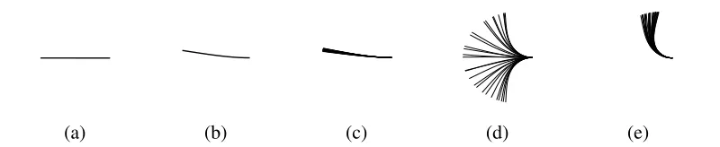
3.5 Illustration of various inverted flag regimes . . . 40

3.6 Vorticity snapshots for an inverted flag . . . 41

4.1 Prediction of the flutter boundary for conventional flag flapping . . . 48

4.2 Global mode of a conventional flag for Mρ=0.05, KB =0.005 . . . 49

4.3 Global mode of a conventional flag for Mρ=1, KB =0.042 . . . 49

4.4 Global mode of a conventional flag for Mρ=50, KB =0.06 . . . 50

5.1 Tip displacement and power-spectral density for small-amplitude limit-cycle flapping of a conventional flag . . . 57

5.2 Snapshots of small-amplitude limit-cycle flapping of a conventional flag . . . 57

(11)

xi 5.4 Leading POD and DMD modes for small-amplitude limit-cycle

flap-ping of a conventional flag . . . 58

5.5 POD and DMD reconstructions of small-amplitude limit-cycle flap-ping of a conventional flag . . . 59

5.6 Tip displacement and power-spectral density of large-amplitude limit-cycle flapping of an inverted flag . . . 59

5.7 Snapshots of large-amplitude limit-cycle flapping of an inverted flag . 60 5.8 POD singular values and DMD eigenvalues for large-amplitude limit-cycle flapping of an inverted flag . . . 61

5.9 Leading POD and DMD modes for large-amplitude limit-cycle flap-ping of an inverted flag . . . 62

5.10 POD and DMD reconstructions of large-amplitude limit-cycle flap-ping of an inverted flag . . . 62

5.11 Tip displacement and power spectral density for large-amplitude limit-cycle flapping and chaotic flapping of a conventional flag . . . . 63

5.12 DMD eigenvalues for for large-amplitude limit-cycle flapping of a conventional flag . . . 64

5.13 Leading DMD modes for large-amplitude limit-cycle flapping of a conventional flag . . . 65

5.14 DMD eigenvalues γ for chaotic flapping of a conventional flag with Re =500,Mρ =0.25,KB = 0.0001. . . 65

5.15 Leading DMD modes for chaotic flapping of a conventional flag . . . 66

7.1 Time lapses for different regimes in inverted-flag flapping . . . 72

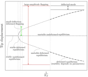
7.2 A schematic bifurcation diagram for inverted-flag flapping . . . 76

8.1 Bifurcation diagrams for inverted-flag flapping with Re= 200. . . 80

8.2 Deformed equilibria of the inverted-flag system forRe =200 . . . . 81

8.3 Frequency response of the inverted-flag system forRe =200 . . . 82

8.4 Leading global modes near the onset of small-deflection deformed flapping for Re =200,Mρ =0.5 . . . 84

8.5 Leading global modes near the onset of small-deflection deformed flapping for Re =200,Mρ =5 . . . 84

8.6 Snapshots of small-deflection deformed flapping . . . 85

8.7 Snapshots of large-amplitude flapping for light flags . . . 86

8.8 Plots of tip displacement and coefficient of lift for light flags . . . 87

8.9 Snapshots of large-amplitude flapping for heavy flags . . . 88

(12)

8.11 Leading global mode for the deflected-mode regime . . . 90 8.12 Plots of tip displacement and spectral density for chaotic flapping of

an inverted flag . . . 91 8.13 Phase portraits demonstrating the strange attractor in chaotic flapping 93 8.14 Bifurcation diagrams for inverted-flag flapping with Re= 20 . . . 95 8.15 Deformed equilibria of the inverted-flag system forRe =20 . . . 96 8.16 Frequency response of the inverted-flag system forRe =20 . . . 96 8.17 Leading global mode of the deformed equilibrium near the onset of

small-deflection deformed flapping for Re =20,Mρ =5 . . . 97 8.18 Leading global mode of the undeformed equilibrium near the onset

(13)

xiii

LIST OF TABLES

Number Page

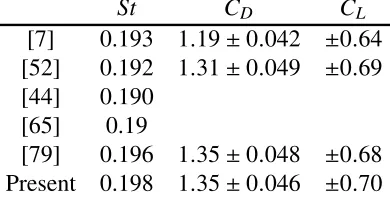
2.1 Shedding frequency for the cylinder in cross-flow problem . . . 23 3.1 Flapping amplitude and frequencies for a conventional flag atRe =1000 36 3.2 Flapping amplitude and frequencies for a conventional flag atRe =200 37 3.3 Flapping regimes of an inverted flag (comparison with the literature) 38 3.4 Flapping amplitude and frequencies for an inverted flag at Re= 1000 40 8.1 Leading-mode growth rate near the onset of small-deflection

de-formed flapping for Re =200 . . . 83 8.2 Leading-mode growth rate near the onset of large-amplitude flapping

for Re =200 . . . 85 8.3 Leading eigenvalues for the deflected-global mode regime . . . 90 8.4 Lyapunov exponents for different regimes of the inverted-flag system 92 8.5 Leading-mode growth rate near the onset of small-deflection

de-formed flapping for Re =20 . . . 95 8.6 Leading-mode growth rate near the onset of large-amplitude flapping

(14)

NOMENCLATURE

χ. Discrete or continuous displacement of the structure immersed in fluid. δ. Dirac-delta function.

δh. Smeared delta function used in immersed-boundary methods.

Γ. Domain defining the structure.

γj. jt h eigenvalue in a dynamic-mode decomposition. ˆ

uj. jt h singular vector in a proper-orthogonal decomposition. ˆ

yj. jt h global mode in a global linear stability analysis.

λj. jt h eigenvalue in a global linear stability analysis.

Ω. Domain defining the fluid. ω. Discrete or continuous vorticity.

σj. jt h singular value in a proper-orthogonal decomposition.

W. Weighting matrix used in defining a norm for proper-orthogonal decompo-sition.

ζ. Discrete or continuous velocity of the structure immersed in fluid.

f. Surface stresses that impose the no-slip boundary condition and drive struc-tural deformation.

KB. Dimensionless flexural rigidity: ratio of structural flexural rigidity to fluid ‘rigidity’.

Mρ. Mass ratio: ratio of structure-to-fluid inertia. p. Fluid pressure.

Re. Reynolds number.

s. Discrete or continuous streamfunction. St. Strouhal number.

(15)

Part I

Numerical methods for

fluid-structure interaction

(16)

C h a p t e r 1

INTRODUCTION

In flow-structure interaction (FSI) systems, fluid moves past an immersed structure and the dynamics of both the fluid and the structure are coupled to one another. High-fidelity numerical simulations can aid experiments and theory in providing physical insights into these systems that can lead to improved bio-inspired propulsion vehicles, medical devices such as heart-valve prosthetics, and renewable energy-harvesting technologies. To this end, a variety of numerical methods have been developed and used to study blood-flow through deformable heart valves [10, 26, 62], flow past flapping flags [17, 26, 32, 82], and insect flight involving passively deforming insect wings [82], to name a few examples.

Of the many methods developed for simulating FSI problems, we focus here on immersed-boundary (IB) methods, which are attractive because they treat the fluid and structure with separate grids and therefore do not involve the computationally expensive task of re-meshing. While IB methods have been extensively developed and used (see Mittal and Iaccarino [56] and Peskin [63] for reviews), there remain open challenges to making them more accurate and efficient. First, many IB meth-ods yield inaccurate surface stresses and forces on the immersed body, both in FSI problems and in rigid-body problems where the structure is either stationary or un-dergoing prescribed kinematics [38, 74, 92]. Second, in FSI problems the nonlinear coupling between the fluid and structure often results in a large nonlinear algebraic system of equations that must be solved iteratively to evolve the FSI system in time (see Hou, Wang, and Layton [34] for a review), and performing these iterations efficiently remains a challenge.

(17)

3 leading edge with respect to the oncoming flow) and the inverted configuration (in which the flag is clamped at its trailing edge).

The method described in chapter 3 is capable of performing high-fidelity simulations that, along with companion simulations and experiments, is a tool for understanding FSI systems. Yet, the dynamics of FSI systems often involve a range of spatial and temporal scales that makes it difficult to identify driving physical mechanisms from simulation or experimental data alone. We therefore devote chapters 4 and 5 to the extension of global stability analysis and snapshot-based data analysis techniques to FSI problems, respectively.

(18)

C h a p t e r 2

ACCURATELY COMPUTING SURFACE STRESSES AND

FORCES WITH IMMERSED BOUNDARY METHODS1

2.1 Introduction

The original IB method of Peskin introduced a singular source term in the momentum equations that imposed the stresses from the immersed body onto the flow grid [62]. In that work, a specific structure was assumed and the surface stresses were derived using the constitutive law for that structure. A different set of IB methods retains the use of a singular source term to impose the surface stresses, but derives these stresses using velocity boundary conditions rather than by directly linking them to deformation of the solid [15, 36–38, 45, 79, 87, 92, 94]. Because they are derived from the boundary conditions on the immersed body, we refer here to these IB methods as surface velocity-based IB methods. These methods produce surface stresses that are poor representations of the physical surface stresses. A subset of these also produce unphysical oscillations in time traces of surface force quantities such as the coefficients of lift and drag, since they enforce the boundary constraint approximately rather than explicitly [36, 87, 94]. Yang et al. [92] reduced the unphysical oscillations in these surface force quantities, but to our knowledge the inaccuracies in the surface stresses have not been addressed. This is likely due to the fact that the velocity field converges in spite of these erroneous surface stresses, so surface velocity-based IB methods may be used without modification for problems where accurate knowledge of the surface stresses is not required.

However, correct information about surface stresses and forces is important in many applications, such as characterizing the performance of wings and aerodynamic bodies in unsteady flows, understanding and controlling flow separation around bluff bodies, and simulating fully coupled flow-structure-interaction (FSI) problems with deforming bodies. In this chapter, we characterize and remedy the spurious surface stresses and forces obtained by surface-velocity based IB methods. We do this in the context of flows past rigid bodies undergoing prescribed kinematics in

1_{This chapter is based on the publication Goza et al. [31], for which my contributions were}

(19)

5 this chapter and the procedure is extended to FSI problems in chapter 3.

It should be noted that there is a class of IB methods called “sharp-interface” meth-ods, which includes ghost-cell [57], cut-cell [86], ghost-fluid [24], and immersed interface methods [49]. While spurious surface stress and force oscillations have been observed for a subset of these methods [53, 75], their cause and remedy is different from what is presented in the current work [53]. A key distinction between this subset of sharp-interface methods and the methods considered here is the use of local flow reconstructions that obviate the need for a singular source term in the momentum equations.

We restrict our attention to methods that contain a singular source term in the momentum equations, and that compute surface stresses and forces using that term. We show that, for any choice of smeared delta function, the equation for the surface stresses is an integral equation of the first kind whose ill-posedness leads to an inaccurate representation of the high frequency components of the surface stresses. The error in these high frequency components was also observed by Kallemovet al. [38] for a six point delta function. We demonstrate that there is an inverse relation between the smoothness of the smeared delta function and the amplitude of the high frequency components for the physically correct stress. Thus, when sufficiently smooth delta functions are selected, the high-frequency components that are erroneously amplified when solving the integral equation may be effectively filtered out of the solution without damaging the overall surface stress. By contrast, filtering out the incorrect high frequency components for insufficiently smooth smeared delta functions obscures important physical information.

(20)

2.2 Demonstrating and resolving inaccurate computation of source terms for a model problem

The difficulty in solving integral equations of the first kind that arise from surface velocity-based IB methods is illustrated and remedied for a model problem in this section. Section 2.3 will demonstrate that the same type of integral equation arises from the Navier-Stokes equations. Thus, the same techniques developed here may be used to compute surface stresses and forces that arise in fluid flows.

The model problem considered is the Poisson equation for an unknown functionψ on a 2D square domainΩ = {x = [x, y]T : |x|,|y| ≤ 1}with an unknown singular source term f that takes nonzero values on an immersed surface denoted byΓ:

∇2ψ(x) =−

Z

Γ

f(χ(s))δ(x−χ(s))ds ψ(x)= ψ∂Ω(x), x∈∂Ω

Z

Ω

ψ(x)δ(x−χ(s))dx= ψΓ(χ(s))

(2.1)

wheresis a variable that parametrizes the IB (e.g., arc length),χ(s)is the Lagrangian

coordinate of a given point on the IB,∂Ωis the boundary of the domainΩ,ψ∂Ω(x)

is a function of prescribed values forψ on∂Ω, and ψΓ₍_χ₍_s₎₎ _{is a function defined}

on the immersed body. Note that the delta function δ(x−χ(s)) is used to relate

quantities between the immersed surface and the solution domain. An error analysis of numerical solutions to (2.1) has been performed in the case where f is prescribed [83, 93]. To mirror surface velocity-based IB methods, we leave f as an unknown that is solved by explicitly incorporating the third equation as a boundary constraint. We takeΓto be a circle of radius 1/2 centered atx= 0,ψ∂Ω(x) = 1− 1₂log(2|x|),

andψΓ₍_χ₎ ₌_{1. The exact solution to (2.1) is then}

ψex(x) =       

1, |x| ≤ 1₂

1− 1₂log(2|x|) |x| > 1₂ (2.2)

fex(χ) =1 (2.3)

Another quantity of interest is Fex =

R

Γ fex(χ(s))ds = π. This term is analogous

to the integrated surface force, which is often of interest for IB flow solvers.

(21)

7 discretized domain on which the numerical solution is obtained (see, e.g., refer-ence [63]). Thus, the numerical solution for a given grid spacing h has as its corresponding continuous solution

ψ(x) =−

Z

Ω

Z

Γ

f(χ(s0))δh(x0−χ(s0))G(x;x0)ds0dx0 (2.4) whereG(x;x0) is the Green’s function for the Poisson problem evaluated atxdue to a source atx0, andδh is the (continuous) smeared delta function. The equation (2.4) is written in terms of the unknown source term f. To arrive at an equation for this source term, we multiply both sides of (2.4) byδh(χ(s)−x)and integrate over the domainΩ:

Z Ω Z Ω Z Γ

f(χ(s0))δh(x0−χ(s0))G(x;x0)δh(x−χ(s))ds0dx0dx=−ψΓ(χ(s)) (2.5) The solutionψ(x)is then obtained by substituting the solution f of (2.5) into (2.4). Sinceδhis continuous for a given grid spacingh, the kernel in the integral equation (2.5) is continuous and has finite support. Thus, the integral operator is compact and formally does not have a bounded inverse [41]. As a consequence, discretizations of this equation lead to inaccurate surface source terms. To highlight that the difficulty in computing the source term occurs for all smeared delta functions, we will use four different functions that are common in the literature. In all cases, the two-dimensional smeared delta function is defined by the tensor product of two one-dimensional smeared delta functions;i.e. δh(x−χ) = δh(x− χ)δh(y−η), where

x= [x,y]T andχ= [χ, η]T_{. The four one-dimensional smeared delta functions we} consider are given below.

• A 2-point hat function:

δhat h (r) =

       1 h− |r|

h2, |r| ≤ h

0, |r|> h (2.6)

• A 3-point function:

δ3 h(r) =

                   1 3h 1+

q

1−3r_h2

!

, |r| ≤ h₂

1 6h 5−

3|r| h −

q

1−31− |r|_h2

!

, h

2 ≤ |r| ≤ 32h

0, |r|> 3₂h

(22)

• A 4 point cosine function:

δcos h (r)=

      

1 4h

1+cos_πr

2h , |r| ≤ 2h

0, |r| > 2h (2.8)

• A Gaussian function:

δG h(r)=

        

q _π

36h2e −π2r2

36h2 , |r| ≤ 14h

0, |r| > 14h

(2.9)

A Gaussian function formally has infinite support. The parameters and cut-off used in (2.9) lead to a truncation error on the order of machine precision. Other parameter choices may be selected to satisfy different error tolerances [93].

To solve the problem numerically, we discretize the system (2.1) as (after replacing the Dirac delta functions with the smeared delta functionsδh)

Lψ = −H f +bL (2.10)

Eψ = ψΓ _(2.11)

where the variablesψ,ψΓ_{, and}

f are understood to be the spatially discrete versions of their continuous counterparts; L is the discrete Laplacian; bL is a boundary condition term that arises from discretizing the Laplacian operator; and H(·) and

E(·)are discretizations of the operations R_Γ(·)δh(x−χ)dsand

R

Ω(·)δh(x−χ)dx,

respectively. Note that the different choices of smeared delta function change E and H. Since E and H have dimensions on the order of the number of solution domain grid points by the number of immersed boundary points, the computational complexity of the algorithm scales linearly with the support of the smeared delta function.

Equations (2.10) and (2.11) may be combined to arrive at an equation for f, given by

(23)

9 The matrix is constructed by solving a Poisson problem for each column of H and then applying the action ofE.

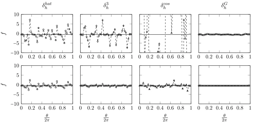
The simulation for this problem was performed using a finite difference discretization on a uniform grid, with the standard 5 point stencil used for L. The grid spacing of the immersed body was chosen to match that of the solution grid. The numerical solution was obtained on the finite domain [−1,1]×[−1,1]; the boundary conditions forψ were obtained by the exact solution (2.2). In what follows, nbandng are the number of points on the immersed body and the solution domain, respectively. Figure 2.1 shows that regardless of the choice of smeared delta function, the source term from (2.12) contains spurious oscillations. Moreover, Figure 2.2 demonstrates that these inaccuracies persist as the grid is refined, so that f does not converge to fex as the grid spacing is decreased. Despite this lack of convergence in f, the integrated source term F and solutionψ converge at first order to Fex and ψex, respectively (see Figure 2.2). Convergence of F is a feature of solving (2.12); methods that enforce the boundary constraint approximately contain inaccuracies inF as well as f [36, 87, 94], though these were improved by Yanget al.[92]. When used with sufficiently smooth smeared delta functions, the method we propose at the end of this section produces convergent approximations for both.

points), and can therefore be stored without difficulty. The matrix is constructed by solving a Poisson problem for each column of H and then applying the action ofE.

The simulation for this problem was performed using a finite di↵erence discretization on a uniform grid, with the standard 5 point stencil used forL. The grid spacing of the immersed body was chosen to match that of the solution grid. The numerical solution was obtained on the finite domain [−1,1] × [−1,1]; the boundary conditions for were obtained by the exact solution (2). In what follows, nb and ng are the number of points on the immersed body and the solution domain, respectively.

Figure 1 shows that regardless of the choice of smeared delta function, the source term from (12) contains spurious oscillations. Moreover, Figure 2 demonstrates that these inaccuracies persist as the grid is refined, so that f does not converge to fex as the grid spacing is decreased. Despite this lack of convergence inf, the integrated source termF and solution converge at first order toFex and ex, respectively (see Figure 2). Convergence ofF is a feature of solving (12); methods that enforce the boundary constraint approximately contain inaccuracies inF as well asf [2, 3, 4], though these were improved by Yanget al.[5]. When used with sufficiently smooth smeared delta functions, the method we propose at the end of this section produces convergent approximations for both.

0 0.2 0.4 0.6 0.8 1

−4 −2 0 2 4 ✓ 2⇡ f hat h

0 0.2 0.4 0.6 0.8 1

✓ 2⇡

3

h

0 0.2 0.4 0.6 0.8 1

✓ 2⇡

cos h

0 0.2 0.4 0.6 0.8 1

✓ 2⇡

G h

Figure 1: Computed source term (f) versus arc length along the cylinder for the Poisson model problem; : fex. All plots usedh=1�640.

As shown in Figure 3, f has the property that Hf does not converge toHfexbut EL−1Hf converges toEL−1_Hf

ex. By virtue of (12), the convergence of EL−1Hf is a statement that using the exact force,fex, to enforce the boundary condition would lead to a boundary value that is not equal to but that converges at first order. This intuitive result was also shown by Tornberg and Engquist [17], and will be exploited in what follows to compute accurate approximations to fex.

To better explain the results of Figure 3, we compute the singular value decomposition (SVD) of EL−1_{. Let} _EL−1 =_U_⌃_VT_{, where} _U ∈_Rnb×nb and V ∈Rng×nb are matrices of left

and right orthonormal singular vectors of EL−1_{, respectively; and ⌃}∈_Rnb×nb is a diagonal

matrix containing the positive singular values of EL−1_{. The singular values}

1, . . . , nb are

5

Figure 2.1: Computed source term (f) versus arc length along the cylinder for the Poisson model problem; : fex. All plots usedh =1/640.

As shown in Figure 2.3, f has the property that H f does not converge to H fexbut

E L−1H f converges toE L−1H fex. By virtue of (2.12), the convergence ofE L−1H f is a statement that using the exact force, fex, to enforce the boundary condition would lead to a boundary value that is not equal to ψΓ _{but that converges at first}

order. This intuitive result was also shown by Tornberg and Engquist [83], and will be exploited in what follows to compute accurate approximations to fex.

(24)

decompo-10−3 ₁₀−2 ₁₀−1

10−4

10−3

10−2

10−1

h

�� − exact��∞

�� exact��∞

10−3 ₁₀−2 ₁₀−1

10−3

100

103

h

��f−fexact��∞

��fexact��∞

10−3 ₁₀−2 ₁₀−1

10−4

10−2

100

h

�F−Fexact� �Fexact�

Figure 2: Errors inf, F, and versus grid spacing (h) for the Poisson model problem. :

hat

h , : h3, : hcos, : Gh, : first order convergence.

arranged such that 1≥ 2≥ ⋅⋅⋅ ≥ nb >0, and the singular vectors are notated such that uj

(vj) is the left (right) singular vector corresponding to j.

10−3 10−2 10−1

10−4

10−2

100

h

��EL−1_H₍_f₋_f_ex)��

∞

��EL−1_Hf_ex��_∞

10−3 10−2 10−1

10−1

101

103

h

��H(f−fex)��∞

��Hfex��∞

Figure 3: Errors inHf andEL−1_Hf _{versus grid spacing (}_h_{) for the Poisson model problem.}

: hat

h , : 3h, : hcos, : hG, : first order convergence.

Using this decomposition, Hfex may be written as a projection onto the basis of vectors

formed byV:

Hfex= nb

�

j=1 ↵ex

j vj (13)

andEL−1_Hf

exmay be expressed as

EL−1_Hf ex=

nb

�

j=1 ↵ex

j juj (14)

where ↵ex

j ∶= (vjTHfex). Analogous expressions exist forHf by replacing fex withf in (13)

and (14). We denote the corresponding coefficients as ↵j∶= (vTjHf).

Using (13) and (14), Figures 3 (a) and (b) show that the sum∑nb

j=1↵j does not converge to

∑nb

j=1↵exj under grid refinement, but does converge when scaled by the j. Since EL−1 is a

6

Figure 2.2: Errors in f, F, and ψ versus grid spacing (h) for the Poisson model problem. : δhat

h , : δ3h, : δ cos h , : δ

G

h, : first order convergence. sition (SVD) of E L−1. LetE L−1 =UΣVT, whereU ∈_Rnb×nb and_V _∈

Rng×nb are matrices of left and right orthonormal singular vectors of E L−1, respectively; and Σ ∈ _Rnb×nb is a diagonal matrix containing the positive singular values of _{E L}−1.

The singular valuesσ₁, . . . , σnb are arranged such thatσ1 ≥ σ2 ≥ · · · ≥ σnb > 0,

and the singular vectors are notated such thatuj(vj) is the left (right) singular vector corresponding toσj.

10−3 10−2 10−1

10−4 10−3

10−2

10−1

h

�� − exact��∞

10−3 10−2 10−1

10−3 100

103

h

��f−fexact��∞

10−3 10−2 10−1

10−4 10−2

100

h

�F−Fexact�

�Fexact�

Figure 2: Errors in f, F, and versus grid spacing (h) for the Poisson model problem. :

hat

h , : h3, : cosh , : hG, : first order convergence.

arranged such that 1 ≥ 2≥ ⋅⋅⋅ ≥ nb >0, and the singular vectors are notated such thatuj (vj) is the left (right) singular vector corresponding to j.

10−3 ₁₀−2 ₁₀−1

10−4

10−2

100

h

��EL−1_H₍_f₋_f_ex_)��_∞ ��EL−1_Hf_ex��_∞

10−3 ₁₀−2 ₁₀−1

10−1

101

103

h

��H(f−fex)��∞

��Hfex��∞

Figure 3: Errors inHf andEL−1_Hf _{versus grid spacing (}_h_{) for the Poisson model problem.}

: hat

h , : 3h, : hcos, : hG, : first order convergence.

Using this decomposition, Hfex may be written as a projection onto the basis of vectors

formed byV:

Hfex= nb

�

j=1 ↵ex

j vj (13)

and EL−1_Hf

ex may be expressed as

EL−1_Hf

ex= nb

�

j=1 ↵ex

j juj (14)

where↵ex

j ∶= (vjTHfex). Analogous expressions exist for Hf by replacing fex with f in (13)

and (14). We denote the corresponding coefficients as↵j ∶= (vT_jHf).

Using (13) and (14), Figures 3 (a) and (b) show that the sum ∑nb

j=1↵j does not converge to

∑nb

j=1↵exj under grid refinement, but does converge when scaled by the j. Since EL−1 is a

6

Figure 2.3: Errors inH f andE L−1H f versus grid spacing (h) for the Poisson model problem. : δhat

h , : δ3h, : δ cos h , : δ

G

h, : first order convergence.

Using this decomposition, H fex may be written as a projection onto the basis of vectors formed byV:

H fex = nb X

j=1

αex

j vj (2.13)

andE L−1H fexmay be expressed as

E L−1H fex = nb X

j=1

αex

j σjuj (2.14)

whereαex j := (v

T

jH fex). Analogous expressions exist forH f by replacing fexwith

(25)

11 Using (2.13) and (2.14), Figures 2.3 (a) and (b) show that the sum Pnb

j=1αj does not converge to Pnb

j=1α ex

j under grid refinement, but does converge when scaled by the σj. Since E L−1 is a discrete integral operator, theσj decay to very small values [33] (see Figure 2.4). Thus, the error in the sumPnb

j=1αjstems from the high index coefficientsαjcorresponding to the smallσj. The key to computing accurate source terms is to use a smeared delta function for which the coefficientsαex

j decay as rapidly as possible. The spurious high index coefficientsαj may then be filtered out to obtain physical source terms. By contrast, it is difficult to accurately compute source terms using smeared delta functions for which theαex

j decay slowly, because the incorrect high indexαj obscure important physical information.

discrete integral operator, the j decay to very small values [21] (see Figure 4). Thus, the error in the sum∑nb

j=1↵jstems from the high index coefficients↵jcorresponding to the small j. The key to computing accurate source terms is to use a smeared delta function for which the coefficients↵ex

j decay as rapidly as possible. The spurious high index coefficients↵j may then be filtered out to obtain physical source terms. By contrast, it is difficult to accurately compute source terms using smeared delta functions for which the↵ex

j decay slowly, because the incorrect high index↵j obscure important physical information.

0 50 100 150 200

10−14

10−9

10−4

101

index (j)

hat h

0 50 100 150 200

index (j)

3 h

0 50 100 150 200

index (j)

cos h

0 50 100 150 200

index (j)

G h

Figure 4: Singular values jofEL−1versus index (j) for the Poisson model problem. A grid spacing ofh=1�80 was used.

Since EL−1 _{is a discrete integral operator, the basis vectors} _v

j are closely related to the standard Fourier basis [21], and (13) behaves like an expansion of Hfex in this basis. The decay rate of the coefficients↵ex

j is therefore governed by the smoothness ofHfex, which is determined by the smoothness of the smeared delta function. This is true becauseHfexis a discretization of_∫_⌦fex(⇠) h(x−⇠)dx, and

d

dx�⌦fex(⇠) h(x−⇠)dx= �⌦fex(⇠)

d

dx h(x−⇠)dx (15)

To demonstrate the e↵ect of the smoothness of the smeared delta function on the decay rate of the coefficients↵ex

j , we consider a sequence of successively smoother delta functions using the recursive formula developed by Yanget al.[5]. Define the operatorS acting on a functiong(r)by

S[g(r)] = � r+1�2

r−1�2 g(˜r)dr˜ (16)

Then the functions we consider are _h3,∗(r) = S[ 3 h(r)],

3,∗∗ h = S[

3,∗

h (r)], and hG, which as a Gaussian may roughly be thought of as the limit of applyingS to 3

h infinitely many times.

Note that 3

h∈C1, 3,∗ h ∈C2,

3,∗∗

h ∈C3, and Gh ∈C∞. Figure 5 shows that the decay rate of the coefficients↵ex

j increases as smoothness of the smeared delta function increases (note the log scale of they-axis). Note that the compactness of a function in Fourier space is roughly

7

Figure 2.4: Singular values σj of E L−1 versus index (j) for the Poisson model problem. A grid spacing ofh =1/80 was used.

Since E L−1 is a discrete integral operator, the basis vectors vj are closely related to the standard Fourier basis [33], and (2.13) behaves like an expansion of H fex in this basis. The decay rate of the coefficients αex

j is therefore governed by the smoothness of H fex, which is determined by the smoothness of the smeared delta function. This is true because H fex is a discretization of

R

Ω fex(χ)δh(x−χ)dx,

and

d dx

Z

Ω

fex(χ)δh(x−χ)dx=

Z

Ω

fex(χ)

d

dxδh(x−χ)dx (2.15) To demonstrate the effect of the smoothness of the smeared delta function on the decay rate of the coefficientsαex

j , we consider a sequence of successively smoother delta functions using the recursive formula developed by Yanget al.[92]. Define the operatorSacting on a functiong(r)by

S[g(r)]=

Z r+1/2

r−1/2

g(r˜)dr˜ (2.16)

Then the functions we consider are δ3_h,∗(r) = S[δ3_h(r)], δ3_h,∗∗ = S[δ_h3,∗(r)], and δG_h,

(26)

infinitely many times. Note that δ3

h ∈ C1, δ 3

h ∈ C2, δ 3

h ∈ C3, and δ G

h ∈ C . Figure 2.5 shows that the decay rate of the coefficientsαex

j increases as smoothness of the smeared delta function increases (note the log scale of they-axis). Note that the compactness of a function in Fourier space is roughly inversely related to its compactness in physical space (see, e.g. [93]), so it is important to pick smeared delta functions whose support is not too narrow.

0 50 100 150

10−14

10−11

10−8

10−5

10−2

101

index (j)

3 h

0 50 100 150

index (j)

3,∗ h

0 50 100 150

index (j)

3,∗∗ h

0 50 100 150

index (j)

G h

Figure 5: Coefficients ↵ex

j for successively smooth smeared delta functions. Obtained using

h=1�80. Note the log scale on they-axis.

inversely related to its compactness in physical space (see, e.g. [18]), so it is important to pick smeared delta functions whose support is not too narrow.

We now discuss the efficient filtering of the spurious high index coefficients ↵j. One may in principle filter out the high index coefficients using the SVD of EL−1_{, but this is a costly} procedure. Instead, we penalize the spurious components off by pre-multiplying it with the matrix ˜EH, where ˜E=EW is a weighted interpolant that takes the smeared source term

Hf back onto the immersed body while preserving its integral value. The filtered source term is then ˜f =EHf˜ . To give the specific form for W, define1= [1,1,�,1]T ∈_Rng×1 and

let(H1)i be theithentry in the vectorH1. ThenW is a diagonal matrix with entries given by

Wii=��

1�(H1)i, (H1)i≠0

0, else (17)

Note that W only applies a nonzero weight if the grid point is within the support of the smeared delta function.

The filter ˜EH redistributes the source term f by convolving it with a kernel of smeared delta functions. The weighting matrix leads to a kernel of the same form as is used in nonparametric kernel smoothing techniques [22], and was inspired from work in this field. As shown below, ˜EH filters the high index coefficients at a rate proportional to the smoothness of the smeared delta function being used. This is due to the fact that ˜EH is itself an integral operator, and therefore the decay rate of its singular values is governed by the smoothness of its kernel [21].

Figure 6 demonstrates the e↵ect of filtering by showing the coefficients ↵ex

j , ↵j and ˜↵j ∶= (vT

jHf˜). Consistent with the observations made above, the high index coefficients ↵j are substantially di↵erent from those of ↵ex

j . For all smeared delta functions, the filtered coef-ficients are better approximations to the exact coefcoef-ficients. Noting that hat

h ∈C0, h3∈C1,

8 Figure 2.5: Coefficientsαex

j for successively smooth smeared delta functions. Ob-tained usingh =1/80. Note the log scale on they-axis.

We now discuss the efficient filtering of the spurious high index coefficientsαj. One may in principle filter out the high index coefficients using the SVD of E L−1, but this is a costly procedure. Instead, we penalize the spurious components of f by pre-multiplying it with the matrix ˜E H, where ˜E = EW˜ is a weighted interpolant that takes the smeared source term H f back onto the immersed body while preserving its integral value. The filtered source term is then ˜f = E H f˜ . To give the specific form for ˜W, define1 = [1,1,· · ·,1]T ∈ _Rng×1and let ₍_H₁₎

i be theit h entry in the vectorH1. Then ˜W is a diagonal matrix with entries given by

˜ Wii =

      

1/(H1)i, (H1)i , 0

0, else (2.17)

Note that ˜W only applies a nonzero weight if the grid point is within the support of the smeared delta function.

(27)

13 due to the fact that ˜E His itself an integral operator, and therefore the decay rate of its singular values is governed by the smoothness of its kernel [33].

Figure 2.6 demonstrates the effect of filtering by showing the coefficients αex j , αj and ˜αj := (vT_jHf˜). Consistent with the observations made above, the high index coefficientsαj are substantially different from those of αex_j . For all smeared delta functions, the filtered coefficients are better approximations to the exact coefficients. Noting thatδhat

h ∈C0, δ3h ∈C1, δ cos

h ∈C0, andδ G h ∈C

∞_{, it is clear from Figure 2.6} that the absolute error in the high frequency ˜αj decreases as the smoothness of the smeared delta function increases. This is because the magnitude of the high index coefficients αex

j is smaller for smoother smeared delta functions, so the spurious high indexαj may be filtered more aggressively.

Figure 2.7 shows the filtered source terms as a function of arc length along the cylinder. By comparison with Figure 2.1, it is clear that the filtered surface stresses are better representations of fex than their unfiltered counterparts. Moreover, note from Figure 2.7 that the approximation to fex improves as the smoothness of the smeared delta function increases. This argument is shown quantitatively by the error plot from Figure 2.8. Indeed, the infinitely differentiableδG

h yields an ˜f that converges to fex. The inability to compute convergent source terms usingδhat_h , δ3_h, andδcos

h stems from the slow decay rate of the coefficientsα ex

j . By contrast, accurate approximations to fex can be obtained for δG_h by simply removing the high index coefficients ofαj.

Note also that it is only the smoothness of the smeared delta functions that matters; δhat

h , δ3h, and δ G

h all satisfy the same number of discrete moment conditions, and the derivative of δ3

h satisfies two more discrete moment conditions than δ G

h. Last, see from Figure 2.8 that filtering does not affect F by virtue of the way ˜E H was constructed, and that the error in the solution ψ is unchanged because computing

˜

f is a post-processing step. For these reasons, we may writeF andψ without the tilde.

It would be desirable to determine a priori the appropriate differentiability of a smeared delta function for a given tolerance in the accuracy of the surface stress. Yet, this is perhaps not possible, as each smeared delta function is associated with a distinct decay rate in singular values and a unique set of singular vectors. For example, δcos

h , δ hat

(28)

sin-14 magnitude of the high index coefficients↵ex

j is smaller for smoother smeared delta functions, so the spurious high index↵j may be filtered more aggressively.

Figure 7 shows the filtered source terms as a function of arc length along the cylinder. By comparison with Figure 1, it is clear that the filtered surface stresses are better represen-tations of fex than their unfiltered counterparts. Moreover, note from Figure 7 that the approximation to fex improves as the smoothness of the smeared delta function increases. This argument is shown quantitatively by the error plot from Figure 8. Indeed, the infinitely di↵erentiable G

h yields an ˜f that converges to fex. The inability to compute convergent source terms using hat

h , h3, and hcos stems from the slow decay rate of the coefficients ↵exj . By contrast, accurate approximations tofex can be obtained for hG by simply removing the high index coefficients of↵j.

Note also that it is only the smoothness of the smeared delta functions that matters; hat h , 3

h, and hG all satisfy the same number of discrete moment conditions, and the derivative of 3

h satisfies two more discrete moment conditions than Gh. Last, see from Figure 8 that filtering does not a↵ectF by virtue of the way ˜EHwas constructed, and that the error in the solution is unchanged because computing ˜f is a post-processing step. For these reasons, we may writeF and without the tilde.

0 50 100 150

10−14

10−11

10−8

10−5

10−2

101

index (j) hat h

0 50 100 150

index (j) 3 h

0 50 100 150

index (j) cos h

0 50 100 150

index (j) G h

Figure 6: Coefficients ↵ex

j (×), ↵j (open markers) and ˜↵j (filled markers) for the Poisson model problem. Note the log scale on they-axis. The grid spacingh=1�80 was used.

It is worth mentioning other possibilities for accurately computing source terms. First, there might be adequately di↵erentiable functions of narrower support than G

h that are sufficiently compact in Fourier space to provide convergent source terms. Second, one may use standard regularization techniques that have been developed for first-kind integral equations, such as

9 Figure 2.6: Coefficientsαex

j (×),αj (open markers) and ˜αj (filled markers) for the Poisson model problem. Note the log scale on they-axis. The grid spacingh=1/80 was used.

0 0.2 0.4 0.6 0.8 1

−4 −2 0 2 4 ✓ 2⇡ ˜_f hat h

0 0.2 0.4 0.6 0.8 1

✓ 2⇡

3

h

0 0.2 0.4 0.6 0.8 1

✓ 2⇡

cos h

0 0.2 0.4 0.6 0.8 1

✓ 2⇡

G h

Figure 7: ˜f vs arc length along the cylinder for the Poisson problem. The exact solutionfex is given by the solid line ( ) for reference.

10−3 ₁₀−2 ₁₀−1

10−4

10−3

10−2

10−1

h

�� − exact��∞

10−3 ₁₀−2 ₁₀−1

10−3

10−2

10−1

100

h

��_f˜₋_f_exact_��_∞ ��fexact��∞

10−3 ₁₀−2 ₁₀−1

10−4

10−2

100

h

�F−Fexact�

�Fexact�

Figure 8: Errors in ˜f,F, and versus grid spacing (h) for the Poisson problem. : hat h , : 3

h, : hcos, : hG, : first order convergence.

Tikhonov reguarization, to compute convergent source terms irrespective of delta function. The difficulty in using these techniques is that they involve a free parameter, and our expe-rience has been that a costly SVD is required to determine this parameter so that the source term converges.

3 Extension to accurately computing surface stresses

and forces

In this section, we consider surface-velocity based IB methods that use a singular source term in the momentum equations. We show that these methods require the solution of a discrete integral equation of the first kind to compute the surface stresses on an immersed body. Therefore, the conclusion that smoother smeared delta functions lead to faster decay of coefficients for the exact surface stresses still holds. Moreover, sufficiently smooth smeared delta functions may be used in combination with the filter ˜EH to obtain surface stresses

10

Figure 2.7: ˜f vs arc length along the cylinder for the Poisson problem. The exact solution fexis given by the solid line ( ) for reference.

0 0.2 0.4 0.6 0.8 1

−4 −2 0 2 4 ✓ 2⇡ ˜_f hat h

0 0.2 0.4 0.6 0.8 1

✓ 2⇡

3

h

0 0.2 0.4 0.6 0.8 1

✓ 2⇡

cos h

0 0.2 0.4 0.6 0.8 1

✓ 2⇡

G h

Figure 7: ˜f vs arc length along the cylinder for the Poisson problem. The exact solution fex

is given by the solid line ( ) for reference.

10−3 ₁₀−2 ₁₀−1

10−4

10−3

10−2

10−1

h

�� − exact��∞

10−3 ₁₀−2 ₁₀−1

10−3

10−2

10−1

100

h

��_f˜₋_f_exact_��_∞ ��fexact��∞

10−3 ₁₀−2 ₁₀−1

10−4

10−2

100

h

�F−Fexact� �Fexact�

Figure 8: Errors in ˜f, F, and versus grid spacing (h) for the Poisson problem. : hat h , : 3

h, : hcos, : hG, : first order convergence.

Tikhonov reguarization, to compute convergent source terms irrespective of delta function. The difficulty in using these techniques is that they involve a free parameter, and our expe-rience has been that a costly SVD is required to determine this parameter so that the source term converges.

3 Extension to accurately computing surface stresses

and forces

In this section, we consider surface-velocity based IB methods that use a singular source term in the momentum equations. We show that these methods require the solution of a discrete integral equation of the first kind to compute the surface stresses on an immersed body. Therefore, the conclusion that smoother smeared delta functions lead to faster decay of coefficients for the exact surface stresses still holds. Moreover, sufficiently smooth smeared delta functions may be used in combination with the filter ˜EH to obtain surface stresses

10

Figure 2.8: Errors in ˜f, F, andψ versus grid spacing (h) for the Poisson problem. : δhat

h , : δ3h, : δ cos h , : δ

G

h, : first order convergence. gular values and exact stress coefficientsαex

(29)

15 Finally, it is worth mentioning other possibilities for accurately computing source terms. First, there might be adequately differentiable functions of narrower sup-port than δG

h that are sufficiently compact in Fourier space to provide convergent source terms. Second, one may use standard regularization techniques that have been developed for first-kind integral equations, such as Tikhonov reguarization, to compute convergent source terms irrespective of delta function. The difficulty in using these techniques is that they involve a free parameter, and our experience has been that a costly SVD is required to determine this parameter so that the source term converges.

2.3 Extension to accurately computing surface stresses and forces

In this section, we consider surface-velocity based IB methods that use a singular source term in the momentum equations. We show that these methods require the solution of a discrete integral equation of the first kind to compute the surface stresses on an immersed body. Therefore, the conclusion that smoother smeared delta functions lead to faster decay of coefficients for the exact surface stresses still holds. Moreover, sufficiently smooth smeared delta functions may be used in combination with the filter ˜E H to obtain surface stresses and forces that converge to the actual stresses and forces on the immersed body.

The nondimensionalized Navier-Stokes equations are considered here on a domain Ωcontaining a body whose boundary is denoted byΓ. The governing equations for surface velocity-based IB methods are written as

∂u

∂t +u· ∇u= −∇p+ 1 Re∇

2_u₊Z

Γ

f(χ(s0,t))δ(x−χ(s0,t))ds0 (2.18)

∇ ·u= 0 (2.19)

Z

Ω

u(x)δ(x−χ(s,t))dx=uΓ(χ(s,t),t) (2.20)

wheref(χ(s0,t)) represents the surface stresses that arise to enforce the boundary

condition (2.20). As with the previous section, all IB methods replace the Dirac delta functions in (2.18) and (2.20) with smeared delta functionsδh.

(30)

integrating over the domain. Doing this gives

Z

Ω

Z

Γ

f(χ(s0,t))δh(x−χ(s,t))δh(x−χ(s0,t))ds0dx=

Z Ω " ∂ ∂t − 1 Re∇

2!_u₍_x₎₊_u_{· ∇}_u₊_∇_p#_δ

h(x−χ(s,t))dx

(2.21)

The key point is that all IB methods replace the delta function with a smeared delta function in the governing equations. Had the Dirac delta function been kept, the integral equation (2.21) would trivially reduce to an expression for the surface stresses f(χ(s,t)). As in (2.5), the integral operator of (2.21) has an unbounded

inverse because it contains a continuous kernel for any finite h.

Many discretizations of (2.18)–(2.20) involve solving a discretized integral equation of the first kind for the surface stresses. Spatially discretizing (2.18)–(2.20) leads to a system of differential algebraic equations given by

˙

u+N(u) =−Gp+ Lu+ H f (2.22)

Du= 0 (2.23)

Eu=uΓ (2.24)

where the overdot denotes differentiation with respect to time;u,p,and f denote the spatially discrete velocity, pressure, and surface stresses; N(u) is a discretization

of the nonlinear term; G, L, and D are discretizations of the gradient, Laplacian, and divergence operators, respectively; andH(·) andE(·)are discretizations of the

operationsR

Γ(·)δh(x−χ)dsand

R

Ω(·)δh(x−χ)dx, respectively.

Consider a time discretization that treats the nonlinear term explicitly and the viscous term implicitly. Then (2.22)–(2.24) become a linear system of equations of the form

        

A G H

D 0 0

E 0 0

                 

un+1

pn+k₁

fn+k₂          =          r₁ r₂ uΓ_n₊₁

         (2.25)

where 0 < k₁,k₂ ≤ 1, A = _∆1_tI − αL (α ∈ _R) comes from the implicit treatment of the viscous term, and r₁ and r₂ are known right hand side terms arising from the explicit time discretization and boundary conditions of the spatial derivative operators.

(31)

17 system such as (2.25) at each stage. If the viscous term were treated explicitly then Awould be replaced with _∆1_tI, though none of the ensuing conclusions would be affected by this change.

Solving (2.25), as is done in the current work, leads to a velocity field that satisfies the boundary conditions on the immersed body at timetn+1[15, 38, 45, 79]. Other surface-velocity based IB methods compute fn+k₂usingun, rather thanun+1[36, 87, 92, 94], which produces a velocity field that does not exactly satisfy the boundary conditions at each time step. We argue in this section that in either case the equation for the surface stresses is an integral equation, and therefore that the results of section 2.2 are valid for either approach.

For the methods that solve (2.25), the equation for the surface stresses may be derived by a block-LU factorization of (2.25) (see reference [79]). Doing this gives

E BH fn+k₂ =r3 (2.26)

wherer₃ is known and B = (A−1G(D A−1G)−1D− I)A−1. The form of B arises because of the time discretization of the system (2.22)–(2.24) and the factorization of (2.25). Equation (2.26) is an approximation of the continuous equation (2.21), and therefore is a discrete integral equation of the first kind. Thus, the logic of section 2.2 applies: smoother delta functions may be used to expand the exact surface stresses on the body using very few terms, and may therefore be combined with the filter ˜E Hto compute accurate surface stresses and forces. It should be mentioned that an analog of the system (2.25) can be formulated in a streamfunction-vorticity formulation [15]. It can be shown that this formulation still leads to a discrete integral equation of the first kind whose kernel is modified from (2.21) by the presence of discrete curl operators. The conclusions of section 2.2 are thus still applicable.

We now show that the methods that useunto compute fn+k₂ also contain an integral equation of the first kind for the surface stresses. In the notation of the current work, the expression for the surface stresses used in references [36, 87, 92, 94] is given by

E H fn+k₂ =

uΓ_n₊₁−Eun

∆t +E(N(un+k3)+Gpn+k4+Lun+k5) (2.27) where 0 ≤ k₃,k₄,k₅ < 1, and all terms on the right hand side are known. This is a discrete integral equation of the first kind whose kernel corresponds to that of (2.21).

(32)

invertible kernel given by the Dirac delta functions. This approximation produces non-convergent surface stresses and forces, though Yanget al.[92] reduced the error in the surface forces. We argue that the root cause of the spurious surface stresses computed by these methods is the nature of the underlying discrete integral equation (2.27), and that the methods of section 2.2 may be used to obtain convergent surface stresses and forces.

Both (2.26) and (2.27) have a time-dependence that was not present in the Poisson problem of section 2.2. For time-dependent problems, the filtering procedure is performed at the end of a given time step. Note also that since the spurious stresses do not affect the accuracy of the velocity field, the filtered stresses do not need to be incorporated into the time-stepping algorithm, even if it requires information of the surface stress at previous time steps (multistep methods) or stages (Runge-Kutta methods). Thus, the time-dependence of the Navier-Stokes equations does not affect the view of the filtering technique as a post-processing procedure.

In the remainder of this paper, we use the IBPM [15] to illustrate that computing surface stresses and forces using the filter ˜E Hleads to increasingly accurate surface stresses as the smoothness of the smeared delta function is increased. We further show that a sufficiently smooth smeared delta function may be used to obtain convergent stresses and forces. These results are demonstrated for multiple test problems.

2.4 An impulsively rotated cylinder

Consider an infinitely long (2-D), infinitely thin cylinder of radiusRin a quiescent fluid that is impulsively brought from rest to constant angular velocityω. Fluid exists inside and outside of the cylinder. All quantities in this section are dimensionless: length scales are nondimensionalized by R, velocities are nondimensionalized by ωR, and time is nondimensionalized byω.

The exact velocity field is in the azimuthal direction, and is given in polar coordinates byuex =uex(r,t)eθ. It may be written as

uex(r,t) =           

r+2P∞

n=1

J₁₍√λ_nr₎ √

λnJ0(

√ λn)e

−λ_{n t}

Re , r ≤ 1

L−1 "

K₁r√sRe

sK₁(√sRe)

#

, r > 1

(2.28)

(33)

19 andL−1[·] represents the inverse Laplace transform with respect to the variables. The exact surface stress is also in the azimuthal direction (fex = fexeθ), and is given by summing the contributions on the inside and outside of the cylinder surface:

fex(t) = 2

Re " ∂

∂r

_u

ex

r

#

r=1−

+ 2 Re

" ∂ ∂r

_u

ex

r

#

r=1+

(2.29)

= 4 Re

∞

X

n=1

e

−λn t

Re + 2

Re " ∂

∂r

_u

ex

r

#

r=1+

(2.30)

The second term on the right hand side of (2.30) is difficult to express analytically by virtue of the inverse Laplace transform in (2.28), but it can be evaluated using numerical routines. Note that the exact stresses are not spatially constant in the Cartesian coordinate system in which the IBPM is formulated, which makes this model problem a more stringent test than if the numerical solution was obtained using a cylindrical polar coordinate system.

The exact surface force in the azimuthal direction (Fex) is obtained by integrating (2.30) along the surface of the cylinder:

Fex(t) =2πfex(t) (2.31)

The inverse Laplace transform was computed using the built-in MATLAB imple-mentation of the Talbot inversion procedure. The inversion is poorly conditioned near the surface of the cylinder, and computations within a radial distance of 0.05 of the cylinder surface were performed in variable precision arithmetic. All quantities in the exact solution (2.28), (2.30), and (2.31) were converged to within 10−10_{. We} compare this exact solution to the IBPM using the smeared delta functions intro-duced in section 2.2. We ran tests for Reynolds numbers ranging from Re = 10 to Re = 200. In the interest of brevity, we primarily show results for Re = 10, with supplementary results given forRe =200.

(34)

the angular velocity of the cylinder was kept at 0.1. In what follows,his defined as the grid spacing on the [−2.5,2.5]×[−2.5,2.5] subdomain.

Figure 2.9 demonstrates that forRe= 10, the filtered stresses are better approxima-tions to fexthan the unfiltered stresses. Morever, the quality of the approximation of the filtered stress is better for smoother smeared delta functions (see also the error in the filtered stresses from Figure 2.10). Indeed, the use ofδG

h leads to filtered surface stresses that converge to the analytical solution fex.

In analogy with section 2.2, the surface forces converge irrespective of smeared delta function (see Figures 2.10 2.11). This is a consequence of solving the discrete integral equation (2.26) to explicitly enforce the boundary condition. The surface velocity-based IB methods that use (2.27) to approximately enforce this condition are known to obtain non-convergent surface forces [92]. Note also that the velocity field converges at first order for all smeared delta functions. In keeping with the notation of section 2.2, tildes are not placed on the variables Fanduto emphasize that these quantities are not affected by the filtering procedure. Figure 2.12 shows the errors in ˜f, F, anduat Re = 200 to highlight the applicability of these results over a range of Reynolds numbers.

anduto emphasize that these quantities are not a↵ected by the filtering procedure. Figure 12 shows the errors in ˜f,F, and uatRe=200 to highlight the applicability of these results over a range of Reynolds numbers.

0 0.2 0.4 0.6 0.8 1

−10 −5 0 5 10 f hat h

0 0.2 0.4 0.6 0.8 1

−10 −5 0 5 10 ✓ 2⇡ ˜_f

0 0.2 0.4 0.6 0.8 1

3 h

0 0.2 0.4 0.6 0.8 1

✓ 2⇡

0 0.2 0.4 0.6 0.8 1

cos h

0 0.2 0.4 0.6 0.8 1

✓ 2⇡

0 0.2 0.4 0.6 0.8 1

G h

0 0.2 0.4 0.6 0.8 1

[image:34.612.98.512.399.600.2]

✓ 2⇡

Figure 9: Top row: tangential surface stress without filtering (f) versus arc length along the cylinder for the rotating cylinder problem atRe=10. Bottom row: filtered surface stresses ( ˜f) versus arc length along the cylinder atRe=10; : fex. All plots usedh=5�200.

10−3 ₁₀−2 ₁₀−1

10−3

100

103

h

��f˜−fexact��∞

10−3 ₁₀−2 ₁₀−1

10−3

10−2

10−1

100

h

�F−Fexact�

�Fexact�

10−3 ₁₀−2 ₁₀−1

10−3

10−2

10−1

100

h

��u−uexact��∞

��uexact��∞

Figure 10: Errors in ˜f, F, and uversus grid spacing (h) for the rotating cylinder problem atRe=10. : hat

h , : h3, : hcos, : hG, : first order convergence.

5 A cylinder in cross-flow

We now consider the canonical problem of flow over an infinitely long (2D) cylinder of diam-eterDthat is impulsively brought to translation at speedU. As with section 4, all quantities

15