A Probabilistic Framework for Real Time Mapping on an Unmanned Ground Vehicle

A Probabilistic Framework for Real-Time Mapping on

an Unmanned Ground Vehicle

Senior Thesis in Control and Dynamical Systems by:

Jeremy H. Gillula

Thesis Advisor:

Professor Joel Burdick

Abstract

Contents

1 Introduction 5

1.1 A Previous Framework and Its Limitations . . . 6

1.2 A Probabilistic Framework . . . 7

2 Technical Approach 9 2.1 Sensor Uncertainty Models . . . 11

2.1.1 LADAR Uncertainty Model . . . 11

2.1.2 Stereovision Uncertainty Model . . . 12

2.1.3 State Estimation Uncertainty Model . . . 14

2.2 The Kalman Filter Framework . . . 16

2.2.1 Cell Update Equations . . . 16

2.2.2 Measurement Discretization . . . 18

2.3 The Disappearing Obstacle Problem . . . 20

3 Implementation and Testing 24 3.1 Experimental Platform . . . 24

3.2 Sensors Used and Verification of Error Models . . . 25

3.3 Experimental Procedure . . . 27

4 Results and Discussion 29 4.1 Map Accuracy and Covariance Characteristics . . . 29

4.2 Data Smoothing Results . . . 31

4.3 Disappearing Obstacle Problem Results . . . 32

4.4 Unanticipated Results . . . 33

5 Conclusions and Future Work 35

List of Figures

1.1 Alice, Caltech’s entry in the 2005 DARPA Grand Challenge. . . 6 1.2 A diagram of the information flow in the software system used on Team

Cal-tech’s 2005 Grand Challenge entry. . . 7

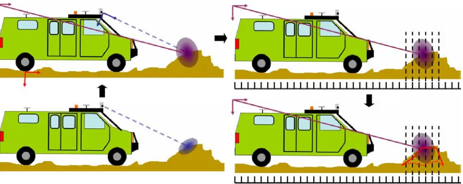
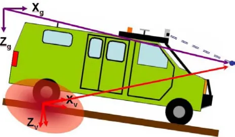
2.1 A diagram of our algorithm – processing proceeds clockwise from the bottom-left. First, a measurement is taken using a sensor and some uncertainty is associated with it using an error model for that sensor. Second, the mea-surement is tranformed into the global coordinate frame, as indicated by the purple axes. (The red axes indicate the intermediary vehicle coordinate frame, as described in the text.) Third, the uncertainty is discretized, as indicated by the dashed lines. Finally, the existing estimate of the elevation in the map, the dashed red line, is fused with the measurement to give a new estimate, the solid red line. . . 10 2.2 The different coordinate frames used throughout this paper, simplified to two

dimensions for easier demonstration. For each of the coordinate frames, the Y axis points out of the page toward the reader. . . 11 2.3 A diagram of how LADAR works: a pulse of light is emitted from the LADAR.

The light then bounces off an object in the environment, and reflects back to a sensor in the LADAR. The time it takes for the pulse to be emitted and then reflected is used to report the range. This procedure is done dozens of times a second as a mirror within the LADAR spins, allowing measurements to be taken in an arc in the robot’s direction of travel. . . 12 2.4 On the left are two images from a stereovision pair, taken of the same scene

2.5 To transform a measurement (the blue dot) from the vehicle frame (the red line pointing to the measurement) to the global frame (the purple line point-ing to the measurement), we must make use of the vehicle’s state estimate to determine where the vehicle is located in the global frame. However, due to errors in the signals from the GPS and IMU, that state estimate is ac-companied by some uncertainty (the faded oval cloud centered on the vehicle frame’s origin, or the offset in the angle between the estimated and actual vehicle frame). . . 15 2.6 The “disappearing obstacle” problem. A long-range sensor detects the

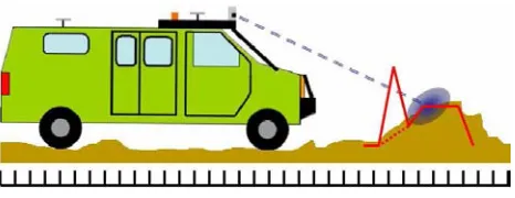
obsta-cle accurately at t = 0. A short-range obstacle then incorrectly states that the obstacle is only as high as the solid line at t = 1, when it is really as tall as the dotted line. At t = 2 the obstacle’s height estimate indicates that it will not be traversable, but it is too late for the vehicle to react and choose another path. . . 20 2.7 Assume the current estimate of the elevation is given by the solid red line, and

the new estimate that would result from fusing in new sensor data is given by the dashed red line. If we then receive a LADAR measurement as shown in blue, there is a high probability that the existing sharp peak in elevation is incorrect, and we should proceed with fusing in the new data. . . 23

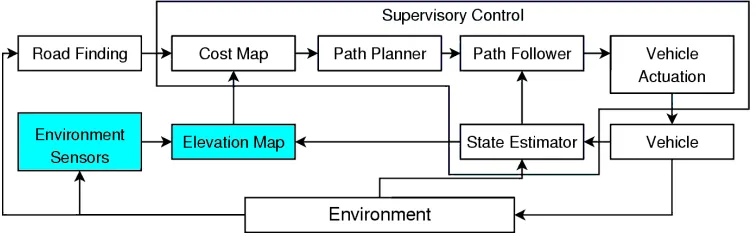
3.1 Alice’s software architecture. The portions relevant to this thesis were the environment sensors (at the bottom left) and the elevation map. . . 24 3.2 Alice’s sensor coverage. The wider cone corresponds to the short-range

stere-ovision; the longer, thinner cone corresponds to the long-range stereovision. The black lines correspond to the intersection of the ground plane with the various scan planes of the LADAR units. The small rectangle is Alice, ap-proximately to scale. . . 25 3.3 Alice, with terrain sensors labeled. (GPS and IMU are not labeled.) . . . 26 3.4 Distribution of scan measurements from a single LADAR unit, in this case

the roof-mounted SICK LMS 221-30206, and the corresponding Gaussian error model. . . 27 3.5 On the left are mean disparity measurements from a set of stereovision images

3.6 Two representative images of the types of desert terrain in which the system was tested. On the left is a sample desert road, lined with small rocks and brush. On the right is a sample dry lakebed, the elevation of which we assumed was completely flat so as to approximate ground-truth. . . 28

4.1 A sample elevation map generated by our algorithm (top) and by individual sensors using the old algorithm (bottom) in conditions for which ground truth is approximately known. The ground-plane (a dry lakebed) is assumed to be flat, and the obstacle (the green blob in the maps) was a 1m by 1m flat board. The elevation of a cell is given by its color — white indicates no data, blue indicates higher elevation, and brown indicates lower elevation, with an overall range of approximately 1m. For scale, the gridlines are 4m apart. . . 29 4.2 A sample covariance map generated by our algorithm. The covariance value

of each cell is indicated by its color. Blue indicates lower covariance, while brown indicates higher covariance. The vehicle’s approximate position and direction of travel are given by the red arrow. The terrain is a relatively flat desert road, with brush on either side. A description of the significance of each labeled region is given in the text. . . 30 4.3 On the left is a sample map generated using the old algorithm, which is dotted

with cells containing no data. On the right is a sample map generated using our algorithm, which has significantly fewer no-data cells. In these maps, the color of a cell corresponds to the estimate of its elevation, with blue cells being higher, red cells being lower, and white cells indicating no data. . . 31 4.4 On the left is a sequence of elevation maps showing the fused map that results

from using the old algorithm, which did not adequately solve the disappearing obstacle problem. On the right is a sequence of maps, taken at the same time steps, illustrating that our method eliminates this problem. . . 32 4.5 An example of data from stereovision overpowering data from a LADAR unit.

The region labeled “B” has been seen by only the LADAR unit, and has a smooth elevation (due to the high accuracy of LADAR). In contrast, the region labeled “A” has been seen by both stereovision and LADAR data, but the elevation in this region is very rough due to the more numerous measurements from stereovision overpowering those of the LADAR, as described in more detail in the text. . . 33 4.6 An example of the data smoothing/obstacle growing that results from using

Chapter 1

Introduction

Autonomous mobile robots (also known as unmanned ground vehicles, or UGVs) have a vari-ety of applications, including use in the military to reduce the risk to soldiers during combat; in industrial settings, especially in autonomous inspections of hazardous waste facilities; and in planetary exploration, of which NASA’s Mars Pathfinder and Mars Exploration Rovers are the most famous examples. However, one of the major limitations of UGVs is the ac-curacy with which they can sense and map their surroundings as they explore, since they must frequently work in unstructured, previously unmapped environments. Complicating the problem further, UGVs must generate maps of their environments using measurements from potentially noisy sensors. Designers frequently attempt to reduce the impact of this problem by using multiple sensor systems with different strengths and weaknesses (Luo and Kay, 1989). Stereovision systems, for example, can provide dense but potetially noisy range data, whereas laser range finders can provide relatively more accurate, but also sparser range data. Using multiple sensors to map an environment brings up two potential problems, how-ever.

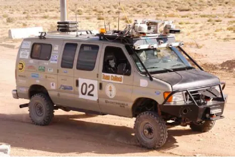
Figure 1.1: Alice, Caltech’s entry in the 2005 DARPA Grand Challenge.

The second question one must answer when using multiple sensors on a UGV is whether or not one can combine the information from the different sensors into a representation of the world that not only makes sense, but is also optimally accurate. In other words, how should one fuse together the data from different sensors? In this thesis we provide an answer to that question, drawing on techniques from control theory to create a probabilistic framework in which to perform sensor fusion.

1.1

A Previous Framework and Its Limitations

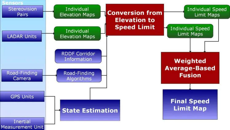
The sensor fusion problem is not a new one, of course, and has been explored in the past. One potential solution was explored by a group of undergraduate and graduate students from Caltech on their entry into the DARPA Grand Challenge: a 10-hour, 175-mile off-road race for unmanned autonomous vehicles that was held for the second time in October 2005 (see figure 1.1). In preparation for the Grand Challenge, a particularly flexible framework was developed for performing sensor fusion, using both DEMs and goodness maps. In particular, every sensor created its own DEM and corresponding goodness map using methods described in Cremean et al. (2006). The resulting goodness maps were then fused using a heuristic algorithm that was biased toward sensors whose coverage areas were closer to the vehicle. A diagram of this framework is depicted in figure 1.2. Unfortunately, this solution had several limitations, which we briefly review here.

Figure 1.2: A diagram of the information flow in the software system used on Team Caltech’s 2005 Grand Challenge entry.

which the range measurements are taken. We describe this problem in more detail in section 2.3.

A second such limitation has to do with what values the goodness map should have in areas which are void of sensor data (no-data areas). There are arguments against both setting the goodness of no-data cells to be high and setting them to be low (again, see Cremean et al. 2006). One potential solution would be to use a probabilistic framework instead, so that meaningful statements could be made about the probability of a given cell having a certain goodness value. Again, this would require a new framework in which to fuse the sensor data.

The final limitation is similar to the no-data limitation described above, in that the system has no confidence data associated with the goodness values (or the elevation values) in a given cell. This limitation was one of the major causes of the failure of Caltech’s vehicle to complete the 2005 Grand Challenge. Essentially, two midrange sensors failed during the course of the race, leaving only a significantly less accurate long-range sensor to guide the vehicle. The vehicle did not slow down while driving through areas of its map about which it should have had less confidence, however, leading it to eventually crash.

1.2

A Probabilistic Framework

limitations described. Although similar sensor fusion algorithms have been proposed before (as in Cremean (2006)), we believe that this is the first system to probabilistically fuse data from disparate sensor types. Thus, the contributions of this thesis are threefold:

1. We present error models for two common types of sensors, stereovision and LADAR (building on results in Ye and Borenstein (2002) and Matthies (1992)), which can then be used in a probabilistic sensor fusion framework.

2. We present a probabilistic framework (inspired by Cremean (2006)) using techniques adapted from control theory (i.e. the Kalman filter), which, given certain conditions on the form of the sensor noise, provide the optimal estimate of the elevation of the surrounding terrain.

Chapter 2

Technical Approach

According to control theory, the optimal estimator for a linear system undergoing Gaussian white noise disturbances is a Kalman filter. Therefore, we would expect that a Kalman filter would perform reasonably well as the means of data fusion for the problem described above. To test this expectation, we implemented a discrete Kalman filter on a cell-by-cell basis for the digital elevation map, with the inputs consisting of the measurements and variances from the different sensors for a given cell, and the output consisting of the estimated elevation and covariance of that cell. The algorithm we propose proceeds as follows, and is depicted graphically in figure 2.1:

1. A range measurement of the terrain surrounding the vehicle is taken, and an error model is used to describe the uncertainty surrounding the measurement.

2. The measurement is transformed into a global coordinate frame, and the uncertainty in the vehicle’s state estimate adds to the uncertainty of the measurement’s position.

3. The measurement (and more specifically, its uncertainty) is discretized so that only a small number of cells in the elevation map need to be updated.

4. In every cell that needs to be updated, the new data is fused by an individual Kalman filter in the particular cell using the discretized information taken from the sensor’s uncertainty model.

One important aspect of this algorithm is that it is performed aysnchronously – data fusion is performed only when new measurements are taken, and no additional processing is required otherwise. Additionally, the computational steps required to perform the data fusion have been developed with an eye toward efficiency, so that the algorithm can perform in real time on a UGV.

Figure 2.1: A diagram of our algorithm – processing proceeds clockwise from the bottom-left. First, a measurement is taken using a sensor and some uncertainty is associated with it using an error model for that sensor. Second, the measurement is tranformed into the global coordinate frame, as indicated by the purple axes. (The red axes indicate the intermediary vehicle coordinate frame, as described in the text.) Third, the uncertainty is discretized, as indicated by the dashed lines. Finally, the existing estimate of the elevation in the map, the dashed red line, is fused with the measurement to give a new estimate, the solid red line.

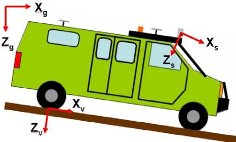
Before we continue, we make note here of the different coordinate systems and notational conventions used throughout the rest of this thesis. In particular, three coordinate frames are used throughout this thesis (figure 2.2):

1. The sensor coordinate frame, which has its origin at a given range sensor. This frame varies from sensor to sensor.

2. The vehicle coordinate frame, which has its origin at ground-level beneath the rear axle of the vehicle, and is oriented such that the x-axis points forward toward the point on ground level beneath the front axle, the y-axis points to the right of the vehicle toward where the right-rear tire touches ground-level, and the z-axis points downward into the ground. This frame moves along with the vehicle.

3. The global coordinate frame, an Earth-fixed reference frame. In this thesis, we make use of the standard UTM (Universal Transverse Mercator) coordinate system, in which the x-axis points north, the y-axis points east, and the z-axis once again points downward into the ground.

To specify in which frame a given variable is being referenced, we frequently use subscripts of the form “descriptor, frame.” So, for example, the x-coordinate of a measurement in the vehicle frame would be referred to by “xm,v”, where the m stands for “measurement” and

Figure 2.2: The different coordinate frames used throughout this paper, simplified to two dimensions for easier demonstration. For each of the coordinate frames, the Y axis points out of the page toward the reader.

For notation, in section 2.1, actual values are denoted with hats (e.g. ρˆ) and Gaussian errors are denoted with tildes (e.g. ρ˜). In sections 2.2 and 2.3, hats are used to denote an estimate of an actual value (e.g. zˆi,j).

2.1

Sensor Uncertainty Models

As was mentioned above, to probabilistically fuse the range measurements from multiple sensors, it is necessary to have both the measurements from the range sensors and the uncertainty estimates associated with each range measurement. We will generate these uncertainty estimates by using statistical error models of the sensors that predict how the sensor’s measurements are affected by noise in the system. We have chosen to present error models for two common types of range sensors used on UGV’s, LADAR (LAser Detection And Ranging) and stereovision. Because the measurements are transformed into the global coordinate system, we also need to take into account the error model of the state sensors, whose output is used to perform the coordinate transformation from the vehicle frame to the global frame.

2.1.1

LADAR Uncertainty Model

LADAR (sometimes referred to as LIDAR) is a name given to a broad category of range sensors which use lasers to precisely determine distances to objects in the sensor’s field of view. Here, we cover LADAR that works on a time-of-flight principle: at a precise time t0,

the sensor emits an infrared laser pulse which is reflected off of a spinning mirror into the environment; that pulse is then reflected by an object back to the sensor, which measures the time t1 at which the pulse returned. The range is then simply ρ = c(t1 −t0)/2 (where

Figure 2.3: A diagram of how LADAR works: a pulse of light is emitted from the LADAR. The light then bounces off an object in the environment, and reflects back to a sensor in the LADAR. The time it takes for the pulse to be emitted and then reflected is used to report the range. This procedure is done dozens of times a second as a mirror within the LADAR spins, allowing measurements to be taken in an arc in the robot’s direction of travel.

If we assume that the noise on both the range and the angle is Gaussian, our error model becomes:

ρ = ˆρ+ ˜ρ (2.1)

θ = ˆθ+ ˜θ (2.2)

whereρ and θ are the reported range and angle measurements, respectively, ˆρ and ˆθ are the true range and angle, and ˜ρ and ˜θ are Gaussian zero-mean random variables that introduce noise into the measurement. This is similar to the model described by Ye and Borenstein (2002), who found an error model for the range of SICK laser scanners (a specific brand and model of LADAR) of the form

ρ = kρˆ+b+ ˜ρ (2.3)

wherekand bare parameters that account for the fact that the reported measurement is not precisely the same as the actual range, but is instead linearly related. In their experiment, they determined that k = 1.0002 and b = 3.6mm. Because these values are negligible compared to the ranges we are measuring1_{, we felt that for our purposes it was safe to}

neglect these terms and use our original error model. For an analysis of how well our model fits the actual LADARs used in the experiment, see section 3.2.

2.1.2

Stereovision Uncertainty Model

In the case of stereovision the error model is somewhat more complex. Stereovision estimates range by making use of two cameras, each mounted on approximately the same backplane a distance b apart from each other, such that the scan lines of each camera are as close to

1_{At the longest possible range reportable by the LADAR units we used in our experiment (81m, according}

Figure 2.4: On the left are two images from a stereovision pair, taken of the same scene simultaneously. The boxes in each image highlight corresponding regions of pixels, and the dashed lines illustrate the different positions the same object has in the two images. By analyzing these differences a disparity image can be created, as shown on the right. In this image, lighter green pixels are closer to the camera, and darker green are further away. Black areas indicate pixels where the algorithm could not confidently make a match, and thus no range was estimated.

parallel as possible. The cameras are then synchronized so that they take images simultane-ously; these images are then fed to a stereovision algorithm, which first warps the images so that their scan lines are exactly parallel using an a priori mapping determined offline using calibration data. The system then analyzes the two images to find similar, or corresponding, regions of pixels. (The methods used to solve this correspondence problem are beyond the scope of this thesis — for a review of such algorithms, see Scharstein and Szeliski (2002).) Once a match is found, the algorithm takes the x coordinate of the central pixel of the matching region in each image, xl and xr, and computes the disparity d =xl−xr. (Figure

2.4.) Through some simple geometry, it can be seen that the range will then be given by

ρ = b×f

d , d={1, . . . , N} (2.4)

where again, b is the baseline (the distance between the two cameras), f is the focal length of the cameras (in pixels), and N is the maximum number of disparities searched. Addi-tional analysis (see Matthies (1992)) shows that the uncertainty inherent in stereovision is fundamentally different from that of LADAR — error in stereovision is proportional to the square of the range and the difference in disparity, and inversely proportional to the focal length and baseline, e.g. if the range is given by

ρ = ˆρ+ ˜ρ (2.5)

then the error is:

˜

ρ ∝ ρˆ

2_∆d

b×f (2.6)

Thus we can model the Gaussian noise ˜ρ as having a variance

ˆ

ρ2_σ

d

where σd is the variance in disparity.

For simplcity we can treat range measurements from stereovision as identical to those from LADAR, despite these differences. We simply treat each scan line from stereovision as we would an individual scan from a LADAR unit, except the pitch of the sensor is now a function of which scan line the measurement comes from. Additionally, we must adjust the error model for each measurement to depend on the reported distance - instead of being a Gaussian of fixed variance regardless of the range reported (as in the LADAR case), we now adjust the variance based on the equation for the error given above. Thus we have:

ρ = ˆρ+ ˜ρ (2.8)

θ = ˆθ+ ˜θ (2.9)

φ = ˆφ+ ˜φ (2.10)

where ρ, θ, and φ are the reported range and angle measurements, respectively, ˆρ, ˆθ, and ˆ

φ are the true range and angles, and ˜ρ, ˜θ, and ˜φ are Gaussian zero-mean random variables that introduce noise into the measurement.

2.1.3

State Estimation Uncertainty Model

To make use of the range information provided by the sensors, we must transform the range measurements into a global coordinate frame so that they can be fused into a global map. This transformation is performed in two steps: first, the range measurement is transformed into the vehicle coordinate frame using calibration data taken offline about the position and orientation of the sensor on the vehicle; second, the range measurement is transformed into the global frame by using position and orientation data provided online by the vehicle’s state estimation system, as in figure 2.5.

If we apply the small angle approximation and neglect second-order terms in the mea-surement noise, the meamea-surement’s location in the vehicle frame (

xM,v yM,v zM,v

T ) is:   xM,v yM,v zM,v   =   xS,v yS,v zS,v  +   ˆ

ρcos ˆθcos ˆφ

ˆ

ρsin ˆθcos ˆφ

−ρˆsin ˆφ



+ (2.11)





cos ˆθcos ˆφ −ρˆsin ˆθcos ˆφ −ρˆcos ˆθsin ˆφ

sin ˆθcos ˆφ ρˆcos ˆθcos ˆφ −ρˆsin ˆθsin ˆφ

−sin ˆφ 0 −ρˆcos ˆφ

    ˜ ρ ˜ θ ˜ φ  

As before, in this expression ˆφis the pitch angle of the measurement with respect to horizon-tal; for LADAR units, this number is a constant for all measurements, while for stereovision systems, it is a function of the scan line of the range measurement.

xS,v yS,v zS,v T

is the location of the sensor in the vehicle coordinate frame.

Figure 2.5: To transform a measurement (the blue dot) from the vehicle frame (the red line pointing to the measurement) to the global frame (the purple line pointing to the measure-ment), we must make use of the vehicle’s state estimate to determine where the vehicle is located in the global frame. However, due to errors in the signals from the GPS and IMU, that state estimate is accompanied by some uncertainty (the faded oval cloud centered on the vehicle frame’s origin, or the offset in the angle between the estimated and actual vehicle frame).

that results from noisy measurements coming from the GPS and IMU). We model these errors as   xV,g yV,g zV,g   =   ˆ xV,g ˆ yV,g ˆ zV,g  +   ˜ xV,g ˜ yV,g ˜ zV,g   (2.12) and   pV,g hV,g rV,g   =   ˆ pV,g ˆ hV,g ˆ rV,g  +   ˜ pV,g ˜ hV,g ˜ rV,g   (2.13) where

xV,g yV,g zV,g T

is the vehicle’s reported position (as determined by the state-estimation software) in the global frame (in which we remind the reader that the x-axis points North, the y-axis points East, and the positive z-axis points downward), and

pV,g hV,g rV,g

T

is the vehicle’s reported pitch, yaw (or heading), and roll with respect to the global co-ordinate frame. As before,

ˆ

xV,g yˆV,g zˆV,g T

and

ˆ

pV,g ˆhV,g rˆV,g T

correspond to the actual values of the corresponding positions and angles, and

˜

xV,g y˜V,g z˜V,g

T

and

˜

pV,g ˜hV,g r˜V,g T

correspond to Gaussian zero-mean random variables that introduce noise into the state estimate.

In general, to transform a measurement from the vehicle coordinate frame to the global coordinate frame, we have:

  xM,g yM,g zM,g 

where

xM,g yM,g zM,g

T

is the measurement’s location in the global coordinate frame, and the rotation matrix is defined by:

R(p, h, r) = (2.15)





coshcosp −cosrsinh+ coshsinrsinp sinrsinh+ cosrcoshsinp

sinhcosp cosrcosh+ sinrsinhsinp −coshsinr+ cosrsinhsinp

−sinp cospsinr cosrcosp





Using these equations, it becomes possible (although algebraically messy) to finally trans-form the measurements and their covariance matrices into the global coordinate frame, taking into account all the uncertainties. Although we omit the actual equations here for brevity, the procedure is outlined as follows:

1. Transform the noisy measurement into the global coordinate frame, to get a vector ~r

inℜ3_.

2. Subtract away what would be the true measurement ~ˆr (e.g. ~r but with all the noise terms set to zero), to get ~r˜=~r−~rˆ.

3. The full 3x3 covariance matrix is then C =~r ~˜r˜T_.

4. To reduce calculation time, we then apply the small-angle approximation in all off the noise terms (since we assume them to be small) and neglect higher-order noise cross terms, giving us ˜C.

The result is a 3x3 matrix which describes the uncertainty ellipse associated with the mea-surement.

2.2

The Kalman Filter Framework

The next step in the algorithm is to fuse the transformed data with existing measurements using a Kalman filter, the details of which are described below.

2.2.1

Cell Update Equations

The basic premise of our Kalman filter framework is that the state we are estimating in each cell is the elevation of that cell,zi,j, where the subscripti, j indicates the location of the cell

in our discrete map. We begin by assuming that the state can be modeled as a standard discrete linear system of the form:

zi,j(k+ 1) = Azi,j(k) +Bui,j(k) +w(k) (2.16)

(2.17)

with a measurement of the form

where zi,j(k) is the state of the system at time k, the matrices A, B, and C represent the

linear model of the plant and the measurements, ui,j(k) is the input to the plant at time

k, yi,j(k) is the measurement taken at time k, and w(k) and v(k) are independent, zero

mean, white, Gaussian random variables that represent the process and measurement noise (respectively), with covariance matricesQ and R.

For this system, the general propagation equations for a discrete Kalman filter are (Welch and Bishop, 2004):

ˆ

zi,j(k+ 1|k) = Azˆi,j(k|k) +Bui,j(k) (2.19)

Pi,j(k+ 1|k) = APi,j(k|k)AT+Q (2.20)

where as is standard, ˆzi,j(k+ 1|k) is the estimate of the state at timek+ 1 given the firstk

measurements, ˆzi,j(k|k) is the estimate of the state at timek given all of the measurements

up to and including those at time k, Pi,j(k+ 1|k) is the estimate error covariance at time

k+ 1 given the first k measurements, and Pi,j(k|k) is the estimate error covariance at time

k given all of the measurements up to and including those at timek.

At this point, it would be possible to make assumptions about the relationship between the elevations of neighboring cells. For example, one could use the dynamic model of the elevation (i.e. the AorB matrices) to apply some sort of smoothness constraint, by relating the elevations of neighboring cells. Within the types of terrain we have encountered experi-mentally, however, we do not believe that any sort of smoothness condition applies; various natural as well as man-made obstacles (such as cliff faces, fence posts, or signs) introduce sudden large discontinuities in elevation which make it difficult to relate the elevation of a given cell to that of its neighbors. (Of course, once a measurement is taken, it is possible to extract information about multiple cells simultaneously - this point is addressed in section 2.2.2.)

Since we have ruled out any relationship between neighboring cells, and since we assume that the environment is static (and since it is not changing, not subject to noise itself) it follows that A= 1, Q= 0, and B = 0. Thus the propagation equations are simply:

ˆ

zi,j(k+ 1|k) = Azˆi,j(k|k) (2.21)

Pi,j(k+ 1|k) = Pi,j(k|k) (2.22)

and so we do not need to perform any time updates. (This is fortunate, because performing some sort of time update to every cell in the map could be extremely computationally expensive, rendering the current algorithm useless in real-time applications.)

We next turn our attention to the measurement update equations. For the system we have described, the general update equations for a discrete Kalman filter are given by (Welch and Bishop, 2004):

ˆ

zi,j(k+ 1|k+ 1) = ˆzi,j(k+ 1|k) +K(k) (zm−Czˆi,j) (2.23)

where zm corresponds to a new elevation measurement for the cell (i, j), and the Kalman

filter gain K is given by:

K = Pi,j(k+ 1|k)CT CPi,j(k+ 1|k)CT+R −1

(2.25)

As with the time update equations, the measurement update equations can be simplified. To begin with, since the coordinate transformations we perform give us immediate access to the elevation of the measurement, we have C = 1. Thus we can write:

ˆ

zi,j(k+ 1|k+ 1) = ˆzi,j(k+ 1|k) +

Pi,j(k+ 1|k) (zm−zˆi,j)

Pi,j(k+ 1|k) +R

(2.26)

= zˆi,j(k+ 1|k) (Pi,j(k+ 1|k) +R) +Pi,j(k+ 1|k) (zm−zˆi,j)

Pi,j(k+ 1|k) +R

= Rzˆi,j(k+ 1|k) +Pi,j(k+ 1|k)zm

Pi,j(k+ 1|k) +R

and

Pi,j(k+ 1|k+ 1) = Pi,j(k+ 1|k)−

Pi,j(k+ 1|k)Pi,j(k+ 1|k)

Pi,j(k+ 1|k) +R

(2.27)

= Pi,j(k+ 1|k)

2_+P

i,j(k+ 1|k)R−Pi,j(k+ 1|k)2

Pi,j(k+ 1|k) +R

= Pi,j(k+ 1|k)R

Pi,j(k+ 1|k) +R

where we remind the reader thatRis the error covariance of the new elevation measurement. In the next section, we explain how we determine R based on the 3D uncertainty ellipsoid of the measurement, ˜C.

2.2.2

Measurement Discretization

Now that we have determined both the measurement mean and the appropriate covariance matrix, as well as how to update a cell given this information, we must choose which cells to update (and how to transform the 3D covariance matrix ˜C into a 1D variance R for use in the Kalman filter). As was indicated in the previous section, for each measurement we will update the estimate of the elevation of multiple cells by taking advantage of the fact that the uncertainty ellipsoid of a single measurement extends over several cells. There are essentially three methods one could use to perform this update.

1. Simply update all the cells in the map with the new measurement.

3. Update cells based on the probability that the measurement came from that cell,

i.e. if the probability that a measurement came from a cell (as determined by the uncertainty ellipsoid generated by the error model) is greater than a given threshold, then we update that cell with the corresponding measurement.

For our implementation we dismissed the first method due to the latency it would in-troduce by requiring an update to every map cell for every single measurement. Instead, we chose to use an update algorithm that combines the second and third methods. In our update algorithm, we calculate which cells have centers that fall within the 95% confidence ellipsoid, and we then update only those cells whose distance from the mean of the measure-ment falls below a given threshold. For our experimeasure-ment, this threshold was set to be 2m, which effectively limited the number of cells updated such that the algorithm could perform in real time on our computing system.

Because we are not estimating a single parameter (like the location of an object in some coordinate system), but are instead discretizing a single measurement so as to estimate several parameters (the elevations of the cells we choose to update), we must also find a way to discretize the covariance we use when we update those cells. In particular, we would like our discretization method to reflect the belief that cells further away from the mean of the measurement are less likely to contain whatever object generated that measurement, and thus should not be as heavily influenced by the measurement. This notion is captured by using the probability functionpi,j(z), which describes the probability that the measurement

actually came from the cell (i, j), from an object of heightz, given the uncertainty ellipsoid of that measurement:

pi,j(z) =

Z Cx(i,j)+∆x 2

Cx(i,j)−∆₂x

Z Cy(i,j)+∆y 2

Cy(i,j)−∆₂y

p(x, y, z)dy dx (2.28)

whereCx(i, j) andCy(i, j) are the xand y coordinates of the center of cell (i, j), ∆x and ∆y

are the width of the cell in the x and y directions (both constants, since we are not using a multi-scale map), and p(x, y, z) is the model of the uncertainty ellipse surrounding the measurement, given by:

p(x) = 1

(2π)3/2pdet ˜C

exp

1

2(x−µ)

T _˜

C−1_(x−µ)

(2.29)

where x= [x y z]T, and µ= [xM,g yM,g zM,g]T, the measurement itself.

Because equation 2.28 cannot be solved analytically, and would be difficult to solve numerically in real time (given that we must makes thousands of updates to cells per second), we instead approximate it by:

pi,j(z) ≈ p(Cx(i, j), Cy(i, j), z)∆x∆y (2.30)

measurement covariance, i.e.:

R = 1

pi,j(zM,g)

(2.31)

2.3

The Disappearing Obstacle Problem

One final topic we will cover is a solution to what we have termed the ”disappearing obstacle” problem. Figure 2.6 is a diagram of this phenomenon; a description follows:

Figure 2.6: The “disappearing obstacle” problem. A long-range sensor detects the obstacle accurately at t = 0. A short-range obstacle then incorrectly states that the obstacle is only as high as the solid line at t = 1, when it is really as tall as the dotted line. At t = 2 the obstacle’s height estimate indicates that it will not be traversable, but it is too late for the vehicle to react and choose another path.

1. t = 0: A long-range sensor detects an obstacle accurately (although with high co-variance), and it is fused into the map as a series of cells with a given height and covariance.

3. t = 2: The obstacle’s correct height is detected by the short-range LADAR, but it is too late for the vehicle to react in time to choose another path.

This phenomenon can occur in any system where there are vertical obstacles such as posts or trees, and close-range sensors with low covariances on their estimates which scan the terrain in a “push-broom” fashion as do LADARs. And while the phenomenon is temporary and the cells are eventually updated to reflect the obstacle’s true height, this correction sometimes does not come quickly enough. In the time it can take for the short-range LADAR to sweep all the way up an obstacle (as the vehicle drives forward), the vehicle’s planning algorithms can attempt to plan a path through the area once occupied by the now vanished obstacle. In fact, this behavior was encountered many times over the course of testing for the 2005 DARPA Grand Challenge; the disappearing obstacle problem frequently caused Alice to attempt to take shortcuts over obstacles it thought for a moment were no longer there, only to find out too late that the obstacle was, in fact, still there.

We make use of the probabilistic nature of our new framework to help solve this problem. In particular, we use a sequential probability ratio test (hereafter referred to as an SPRT) to determine whether or not the new measurements coming from the short-range LADAR should be fused into, and in some sense replace, the existing data in a given cell. For every new measurement that comes into a non-empty cell, we test the simple hypothesis that either:

H0: The new data corresponds to the same obstacle previously detected in that cell, and

fusing the new data with the old data will not cause the existing obstacle to disappear, or,

H1: The new data does not correspond to the same obstacle previously detected in that

cell, but it will result in a more accurate estimate of the elevation of that cell (i.e. the old data was inaccurate and should be replaced).

In either case, if the hypothesis is proven true then the proper course of action is to fuse in the new data.

Of course, we can determine which of H0 orH1 is true simply by examining the values of

the new measurements. If they are “close” to the existing value then we can be fairly sure

H0 is true. If they are “far” from the existing value, then the old data is probably inaccurate

and H1 is likely to be true. We will determine whether the measurements are “close” by

testing whether or not they correspond to a normal distribution with mean given by the existing estimate, and variance given by the variance in elevation of the measurements that have been fused into that cell, weighted by their covariance. This variance is given by

σ2

i,j =

Pn k=0

Rk(ˆzi,j −zM,gk)2

PN k=0Rk

(2.32)

wherenmeasurements (zM,g1, . . . , zM,gn) have fallen into the cell (i, j), whose current estimate

Now that we have the mean (ˆzi,j) and variance (σi,j), we can proceed to describe the

specific SPRT we perform. Following Wald (1947), we note that the probability density of a sequence of n measurements of the elevation of the cell (zM,g1, . . . , zM,gn) under our

hypothesis is:

p0n =

1 (2π)n2 σn

i,j

exp − 1 2σ2

i,j n X

i=1

(zM,gi−zˆi,j)2 !

(2.33)

According to Wald (1947), we want to compare this probability density to a probability density p1n which is a weighted average of the probability density corresponding to various

values of zi,j for which we would reject H0. As derived in Wald (1947), an optimal choice

for p1n is:

p1n =

1 2 (2π)n2 σn

i,j

exp − 1 2σ2

i,j n X

i=1

(zM,gi −zˆi,j+δσi,j)2 !

+ (2.34)

1 2 (2π)n2 σn

i,j

exp − 1 2σ2

i,j n X

i=1

(zM,gi −zˆi,j−δσi,j)2 !

which is simply the average of the two density functions corresponding to zi,j = ˆzi,j +δσi,j

and zi,j = ˆzi,j−δσi,j, where zi,j is the actual value of the elevation of the cell (i, j), andδ is

given by: ˆ

zi,j −zi,j

σi,j

≥ δ (2.35)

where we wish to reject the hypothesis H0 if this inequality is true. Of course, rejecting H0

is equivalent to accepting H1.

Then, for some thresholds A and B, the test would normally be carried out as follows:

1. When a new measurement of a cell comes in, check to see if any data already exists in that cell. If less than two data points have been used to estimate the state of the current cell, fuse in the new measurement immediately. Otherwise:

2. Calculate p1n/p0n, as given by equations 2.34 and 2.33.

(a) If p1n/p0n ≤B, accept H0, and fuse in all of the data in the current cell’s buffer

using the Kalman filter procedure described in equations 2.26 and 2.27, and keep track of the variance in elevation using equation 2.32.

(b) If p1n/p0n ≥ A, accept H1, and fuse in all of the data in the current cell’s buffer

using the Kalman filter procedure described in equations 2.26 and 2.27, and keep track of the variance in elevation using equation 2.32.

(c) If B ≤ p1n/p0n ≤ A, add the measurement to the buffer and continue taking

Figure 2.7: Assume the current estimate of the elevation is given by the solid red line, and the new estimate that would result from fusing in new sensor data is given by the dashed red line. If we then receive a LADAR measurement as shown in blue, there is a high probability that the existing sharp peak in elevation is incorrect, and we should proceed with fusing in the new data.

One can see that since the acceptance of either hypothesis leads to the same action, the SPRT essentially serves as a mechanicsm to delay fusion of new range data. One possible drawback to this approach is that it could result in the delayed detection of obstacles in cases where the old data did not detect the obstacle, but the new, delayed data does. Despite this, we believe that this drawback will be less dangerous than the disappearing obstacle problem which the SPRT seeks to solve.

Chapter 3

Implementation and Testing

To test the algorithm we have described, we implemented it within the framework of Team Caltech’s entry in the 2005 DARPA Grand Challenge, Alice. In this section, we describe in more detail the various hardware and software used for this implementation; most of this information is also available in Cremean et al. (2006), which is more broadly focused.

3.1

Experimental Platform

Alice, the UGV used for testing, is a Ford E350 van modified by Sportsmobile West of Fresno, CA, for off-road operations. While the hardware modifications that allow Alice to perform autonomously off-road are nontrivial and required a significant amount of effort, for the purposes of this thesis they are not nearly as important as Alice’s software architecture. Thus, for more information on the hardware aspects of the testing platform, we direct the reader to Cremean et al. (2006).

The software system used on Alice was designed to be modular and easily adaptable (see figure 3.1). Each sensor has a dedicated software module known as a “feeder,” which reads in data from that sensor over a physical connection (such as a USB or IEEE 1394 port), and then broadcasts that data to Alice’s internal LAN, where it can be received by any

Figure 3.2: Alice’s sensor coverage. The wider cone corresponds to the short-range stereo-vision; the longer, thinner cone corresponds to the long-range stereovision. The black lines correspond to the intersection of the ground plane with the various scan planes of the LADAR units. The small rectangle is Alice, approximately to scale.

other software module running on a computer connected to the network. One such module is the mapping module, which then combines the data from the different sensors into a single cost map of Alice’s environment. The cost-map itself, as well as the elevation maps, are implemented using a scrolling framework in which the vehicle is always located at the center of the map, and the edges of cells are oriented along the northing-easting coordinate system. That cost-map is then broadcast to the vehicle’s path planning module, which uses the map to compute an appropriate path. Although communications between the various components of the system are based on message passing over a gigabit Ethernet network, we did not encounter any problems with dropped packets or lack of bandwidth. Throughout the experiment, we used maps that were 200m on a side, with cells that were 40cm on a side.

3.2

Sensors Used and Verification of Error Models

Prior to the 2005 DARPA Grand Challenge, members of Team Caltech, with help from the Aluminess company, outfitted Alice with several sets of semi-redundant sensors. For a complete description of the sensors used, see table 3.1; figure 3.2 shows the coverage of the sensors on flat, level terrain; figure 3.3 shows where the sensors are actually located on Alice. Of course, it was necessary to verify that the sensor error models we presented earlier were accurate, i.e., that they had the statistical properties we assumed. To ensure this, we collected large samples of data points from both types of sensors, and then analyzed their statistical properties. The results, shown in figures 3.4 and 3.5, demonstrate that our assumptions hold.

Sensor Type Mounting Location Specifications LADAR (SICK LMS

221-30206)

Roof 180◦ _{FOV, 1}◦ _{resolution, 75Hz, 80m}

max range, pointed 20m away LADAR (SICK LMS

291-S14)

Roof 90◦ _{FOV, 0.5}◦ _{resolution, 75Hz, 80m}

max range, pointed 35m away

LADAR (Riegl LMS Q120i) Roof 80◦ _{FOV, 0.4}◦ _{resolution, 50Hz, 120m}

max range, pointed 50 m away LADAR (SICK LMS

291-S05)

Bumper 180◦ _{FOV, 1}◦ _{resolution, 80 m max}

range, pointed 3m away LADAR (SICK LMS

221-30206)

Bumper 180◦ _{FOV, 1}◦ _{resolution, 80m max}

range, pointed horizontally Stereovision Pair (Point

Grey Dragonfly)

Roof 1 m baseline, 640x480 resolution, 2.8 mm focal length, 128 disparities

Stereovision Pair (Point Grey Dragonfly)

Roof 1.5 m baseline, 640x480 resolution, 8 mm focal length, 128 disparities

Road-Finding Camera (Point Grey Dragonfly)

Roof 640x480 resolution, 2.8mm focal length

IMU (Northrop Grumman LN-200)

Roof 1–10◦ _{gyro bias, 0.3–3 mg acceleration}

bias, 400 Hz update rate GPS (Navcom SF-2050) Roof 0.5 m CEP, 2 Hz update rate GPS (NovAtel DL-4plus) Roof 0.4 m CEP, 10 Hz update rate

Table 3.1: The various terrain sensors used on Alice on the day of the Grand Challenge. Not all of these sensors were used at all points during the current experiment.

Figure 3.4: Distribution of scan measurements from a single LADAR unit, in this case the roof-mounted SICK LMS 221-30206, and the corresponding Gaussian error model.

In figure 3.5, we have plotted the mean and standard deviations of the disparity (averaged over more than one hundred images). The overall variance of the disparity for the pixels in the image was σd= 0.7256.

3.3

Experimental Procedure

To test the final system, we drove the UGV manually through two different types of terrain, as depicted in figure 3.6. The first type of terrain was a flat dry lakebed, populated by obstacles comprised of simple geometric shapes where ground-truth was approximately known, so that we could perform calibrated tests on the accuracy of our system’s ability to properly estimate elevation. The second type of terrain was a more realistic desert environment which was chosen so as to verify that our algorithm would successfully achieve three goals:

1. Comparable accuracy in elevation to the old algorithm, along with reasonable covari-ance values.

2. Reduced areas of no data in comparison to the old algorithm.

3. Elimination of the disappearing obstacle problem.

For this terrain, which was composed of a bumpy dirt road along with obstacles such as sage brush and small rocks, ground truth was not known, so only qualitative comparisons were made.

Mean Disparity Values

100 200 300 400 500 600 −100 −50 0 50 100 150 200 250 300 350 0 10 20 30 40 50 60 70 80

90 Variance Values

100 200 300 400 500 600 −100 −50 0 50 100 150 200 250 300 350 0 0.5 1 1.5 2 2.5 3 3.5 4

Figure 3.5: On the left are mean disparity measurements from a set of stereovision images taken by the short-range (1m baseline) pair while the vehicle was stationary. The disparity of each pixel is indicated by its color, according to the colorbar on the right. On the right is the variance in disparity at each pixel. Again, the value of the variance at each pixel is indicated by its color, according to the colorbar on the right. In both cases, dark blue pixels at the bottom of the scale indicate no disparity was estimated by the stereovision algorithm due to lack of texture in the image. At the bottom is a sample image from the sequence used during this test.

Chapter 4

Results and Discussion

Our major results are fourfold, and are described below. First, in section 4.1, we show that our algorithm generates maps with the elevation and covariance values we would expect given the different sensors that have filled in the map. Second, in section 4.2, we show that our algorithm dramatically reduces the “no data” problem. Third, in section 4.3 we show that our algorithm successfully solves the “disappearing obstacle” problem. Finally, we close with section 4.4 by mentioning a few unanticipated results of our algorithm.

4.1

Map Accuracy and Covariance Characteristics

Figure 4.1 shows a sample elevation map generated as a result of our algorithm. The estimated height of the obstacle, which is 1m tall, is approximately 50cm. This disparity is to be expected — our algoirhtm fuses together all of the range data from the obstacle (from its top to its bottom) and so the resulting height estimate is close to the obstacle’s mean elevation. We also note that the obstacle appears much larger in the map than it actually is — this phenomenon is explained in more detail in section 4.4. The height estimates in the individual elevation maps (shown on the bottom) are comparable, indicating no degradation in performance from the use of our framework.

Figure 4.2: A sample covariance map generated by our algorithm. The covariance value of each cell is indicated by its color. Blue indicates lower covariance, while brown indicates higher covariance. The vehicle’s approximate position and direction of travel are given by the red arrow. The terrain is a relatively flat desert road, with brush on either side. A description of the significance of each labeled region is given in the text.

Figure 4.2 shows a sample covariance map generated as a result of our algorithm. For this example we used the short-range (1m baseline) stereovision pair, as well as the roof-mounted SICK LMS 221-30206 and SICK LMS 291-S14. Of course, our algorithm is not limited to using only three different sensors — in this example we used only three for simplicity of presentation. In particular, one can pick out which regions were filled in by which sensors based on the values of the covariance in those regions, as described below:

Region B: This light-blue region was generated by coverage of both the short- and long-range LADAR units, but not the stereovision pair. Thus the covariance is slightly higher than that in region A.

Region C: This darker region was generated as a result of multiple scans by the short-range LADAR of the same patch of ground due to the vehicle being stationary. Because more measurements have been taken, the covariance is lower than that of region B.

Region D: This lighter region has been seen only by the long-range LADAR, thus it has the highest covariance of any area in front of the vehicle.

Region E: As with region C, this region is slightly darker than region D (and thus has a lower covariance) because the long-range LADAR was able to take multiple scans of this area due to the vehicle being stationary.

Region F: The spotty regions to either side of the road the vehicle is traveling on are a result of measurements of nearby brush. Because measurements are less dense to the sides of the vehicle than directly in front of the vehicle, the covariance is the highest in these areas.

4.2

Data Smoothing Results

Figure 4.3: On the left is a sample map generated using the old algorithm, which is dotted with cells containing no data. On the right is a sample map generated using our algorithm, which has significantly fewer no-data cells. In these maps, the color of a cell corresponds to the estimate of its elevation, with blue cells being higher, red cells being lower, and white cells indicating no data.

better in that its “interpolation” is performed probabilistically as a function of the incoming measurements, and makes no assumptions about the smoothness of the map.

4.3

Disappearing Obstacle Problem Results

t= 0

t= 5

t= 7

Figure 4.4: On the left is a sequence of elevation maps showing the fused map that results from using the old algorithm, which did not adequately solve the disappearing obstacle problem. On the right is a sequence of maps, taken at the same time steps, illustrating that our method eliminates this problem.

while it is preserved in the map on the right. Finally, at t = 7, the vehicle has passed the obstacle and it has reappeared in both maps. Although the algorithm performed correctly on this specific set of data, there were cases for which the obstacle still disappeared (albeit to a smaller extent than before we began using the SPRT). Additionally, a great deal of trial-and-error was involved in choosing values of A, B, and δ which would result in the algorithm performing correctly.

4.4

Unanticipated Results

Finally, we close this section by noting some interesting unanticipated characteristics of our solution to the elevation-fusion problem not mentioned above.

Figure 4.5: An example of data from stereovision overpowering data from a LADAR unit. The region labeled “B” has been seen by only the LADAR unit, and has a smooth elevation (due to the high accuracy of LADAR). In contrast, the region labeled “A” has been seen by both stereovision and LADAR data, but the elevation in this region is very rough due to the more numerous measurements from stereovision overpowering those of the LADAR, as described in more detail in the text.

that number is rarely higher than two or three. Additionally, for a given frame the measure-ments from stereovision that fall into a single cell tend to be highly correlated. (In other words, the Gaussian noise occurs between the disparity values a pixel has in separate im-ages, not between the disparity values individual pixels have within a single image.) Thus, when the fusion is performed, the more numerous and highly correlated measurements from stereovision tend to outweigh the measurements generated via LADAR. While this does not necessarily represent a flaw in the system, it may be desirable to investigate an alternative error model for the stereovision system that takes into account the highly correlated nature of the measurements generated by stereovision for a given image.

Figure 4.6: An example of the data smoothing/obstacle growing that results from using our algorithm. The growing phenomenon (which is described in the text) makes the obstacles indicated by the red arrows appear larger in the map than they are in reality.

Chapter 5

Conclusions and Future Work

In this thesis we have presented a probabilistic framework for performing real-time mapping aboard an unmanned ground vehicle. Our framework has successfully solved some of the problems that plagued the previous heuristic solution used by Team Caltech on its 2005 DARPA Grand Challenge entry. In particular, we have presented error models for two dif-ferent types of range sensors, and made use of Kalman filters to fuse together elevation measurements from those different sensors using their corresponding error models. Addi-tionally, we have added safeguards that take advantage of the probabilistic nature of our framework to prevent obstacles from temporarily disappearing from the map. The resulting algorithm solves the “disappearing obstacle problem,” reduces the number of “no-data” cells in the map, and provides a covariance map which indicates the algorithm’s confidence in each cell’s estimated elevation.

A problem we have not covered in this thesis, but which is of critical importance within the overall software architecture used by Caltech’s vehicle, is the problem of how to convert elevation maps into goodness maps. For the 2005 Grand Challenge, a heuristic method was used to convert elevation maps into goodness maps. However, due to the heuristic nature of the elevation fusion, no confidence data was available for use during this conversion, and so Alice drove at the same speed through terrain seen with its less accurate long-range sensors as it did through terrain seen with its more accurate short-range sensors. In fact, this lack of distinction between which sensors had seen (or not seen) the terrain surrounding Alice was one of the major causes of the Caltech vehicle’s failure to complete the 2005 Grand Challenge. By incorporating the covariance values generated by our algorithm (e.g., by setting cells with a high covariance to have a lower goodness, and vice versa) this sort of failure can be avoided in the future, and we strongly recommend that this adaptation be investigated in future research.

obstacle exists.

Another major such extension would be to use a multi-resolution map for storing the el-evation data — that is, a map that does not have a fixed resolution, as ours did, but instead automatically subdivides into smaller cells as new measurements are taken and smaller fea-tures are detected. Alternatively, one could abandon the discretized nature of a grid-based map altogether, and attempt to group measurements together into individual obstacles or features that were not restricted to specific grid cells, but whose positions and other charac-teristics were instead freely estimated using the incoming range measurements. In essence, this framework would model the world in a vectorized manner, as opposed to the rasterized model we have used.

Before we conclude, there is one final issue which we feel needs to be addressed given the overall framework within which the research presented in this thesis fits. In particular, this thesis has been the culmination of several years of work on the 2004 and 2005 DARPA Grand Challenges. Recently, however, DARPA has announced a third Grand Challenge, to be held in November 2007, which will focus primarily on autonomous driving in urban, dynamic environments. It is clear that this urban Grand Challenge (DGC3) will present difficulties that are somewhat different from those of the previous two Grand Challenges (DGC1-2). The most notable difference, of course, is that in DGC1-2, the assumption that the environment would be static was a valid one, whereas in DGC3, the environment will be dynamic, i.e., it will contain moving obstacles such as other vehicles. Because this static assumption was critical for the mapping framework developed for DGC1-2 and presented here, it is clear that additional work will be required for the Team Caltech vehicle to be able to compete in DGC3. In particular, we believe that navigation in an urban environment will require the vehicle to have a great deal more understanding and awareness of its environment. It will no longer be adequate for the vehicle to treat all terrain features the same based solely on their rough geometry, e.g., treating vehicles and large boulders the same, since they have roughly the same overall size and shape in an elevation map. Instead, the vehicle will have to actively recognize objects like vehicles, and attempt to model their dynamics to predict how they will behave. The rasterized mapping framework used for DGC1-2 may not be sufficient for this aspect of DGC3; a framework closer to the vectorized one described in the previous paragraph may be needed.

Chapter 6

Acknowledgements

First and foremost, I would like to thank my thesis advisor, Professor Joel Burdick, for be-ing an extremely patient and flexible mentor over the course of this project. I also want to thank Professor Richard Murray for his inspiration and leadership — without his support, this thesis (not to mention a lot of other research projects) never would have happened. Additionally, I want to thank Professor Pietro Perona for his assistance and advice over the course of the DARPA Grand Challenge. Finally, I want to thank all three of these men for all of their advice on matters both inside and outside the technical realm — their insight and support has been invaluable throughout my undergraduate career.

I also wish to thank all of my friends on Team Caltech who helped make Alice (and Bob!) possible, especially: Lars Cremean, Kristo Kriechbaum, Sam Pfister, Alex Stewart, Dima Kogan, and Joe Donovan. Most of all, I want to especially recognize Tony and Sandie Fender, without whose support the team would have collapsed from starvation and heat exhaustion long ago.

And last, but not least, thank you Alice, for never letting us down.

Bibliography

Bellutta, P., Manduchi, R., Matthies, L., Owens, K., and Rankin, A. (2000). Terrain percep-tion for DEMO III. InProceedings of the 2000 Intelligent Vehicles Conference, Dearborn, MI.

Cremean, L. B. (2006). System Architectures and Environment Modeling for High-Speed Autonomous Navigation. PhD thesis, Caltech.

Cremean, L. B., Foote, T. B., Gillula, J. H., Hines, G. H., Kogan, D., Kriechbaum, K. L., Lamb, J. C., Leibs, J., Lindzey, L., Stewart, A. D., Burdick, J. W., and Murray, R. M. (2006). Alice: An information-rich autonomous vehicle for high-speed desert navigation.

Journal of Field Robotics.

Goldberg, S., Matthies, L., and Maimone, M. (2002). Stereo vision and rover navigation software for planetary exploration. InProceedings of the 2002 IEEE Aerospace Conference, Big Sky, MT.

Luo, R. and Kay, M. (1989). Multisensor integration and fusion in intelligent systems. IEEE Transactions on Systems, Man, and Cybernetics, 19(5):901–931.

Matthies, L. (1992). Toward stochastic modeling of obstacle detectability in passive stereo range imagery. In Proceedings of the IEEE Computer Society Conference on Computer Vision and Pattern Recognition, Champaign, IL.

Scharstein, D. and Szeliski, R. (2002). A taxonomy and evaluation of dense two-frame stereo correspondence algorithms. International Journal of Computer Vision, 47(1-3):7–42. Wald, A. (1947). Sequential Analysis. Wiley Publications in Statistics. John Wiley and Sons,

Inc., New York.

Welch, G. and Bishop, G. (2004). An introduction to the kalman filter. Technical Report 95-041, University of North Carolina at Chapel Hill.