Towards a UTP style framework to deal with probabilities

(1)

Towards a

UTP

-style framework

to deal with probabilities

Riccardo Bresciani, Andrew Butterfield

★

Abstract We present an encoding of the semantics of the probabilistic guarded command language (pGCL) in the Unifying Theories of Programming (UTP) framework. Our contribution is aUTPencoding that capturespGCL pro-grams as predicate-transformers, on predicates over probability distributions on before- and after-states: these predicates capture the same information as the models traditionally used to give semantics topGCL; in addition our formu-lation allows us to define a generic choice construct, that covers conditional, probabilistic and non-deterministic choice. We introduce the concept of prob-abilistic refinement in this framework. This technical report gives a rigourous presentation of our framework, along with a variety of proofs and examples (including the well-known Monty Hall problem), that help to explain it.

1 Introduction

Formal program verification allows us to prove that a program complies with its specification and that it does not generate faulty behaviour of any kind, and in general that certain properties hold when a given program is run.

This aim is achieved by writing a model of the program and subsequently verifying the model. Nonetheless this provides no information regarding the probability that a property will hold: some-times it is more useful to know what are the odds that a property holds, rather than “simply” assert that it does not always hold.

The purpose of this work is to develop aUTP1_{-style framework where we can express probabilistic}

programs, featuring both probabilistic choice and non-determinism: we aim at being able to do inUTPall of the things that are feasible inpGCL2_{. UTP is based on (state-)predicate transformers,}

whereas probabilistic models typically involve distributions over states, and so the best way to integrate probability into theUTPframework is not obvious.

We aim at constructing a theory of probabilistic programs that is expressed using predicate-transformers3_.

1.1 UTP

: general principles

The Unifying Theories of Programming (UTP) research activity seeks to bring models of a wide range of programming and specification languages under a single semantic framework in order to be able to reason formally about their integration [HJ98; DS06; But10; Qin10]. A success in this area has been the development of theCircus language [OCW09], which is a fusion of Z and CSP, with aUTPsemantics, providing specifications using a “state-rich” process algebra along with a refinement calculus; recent extensions toCircus have included timed [SH03] and synchronous [GB09] variants. Recent interest in aspects of the POSIX filestore case study in the Verification Grand Challenge [FWB08] has led us to consider integrating probability intoUTP, with a view to eventually having a probabilistic variant ofCircus.

Theories inUTP are expressed as second-order predicates4 _{over a pre-defined collection of free}

observation variables, referred to as thealphabetof the theory. The predicates are generally used to describe a relation between a before-state and an after-state, the latter typically characterised by dashed versions of the observation variables. For example, a program using two variablesxand ymight be characterised by having the set{x, x′, y, y′}as an alphabet, and the meaning of the

assignmentx∶=y+4would be described by the predicate x′=y+4∧y′=y.

In effectUTP uses predicate calculus in a disciplined way to build up a relational calculus for reasoning about programs.

In addition to observations of the values of program variables, often we need to introduce obser-vations of other aspects of program execution via so-called auxiliary variables. So, for example, in order to reason about total correctness, we need to introduce boolean observations that record the starting (ok) and termination (ok′) of a program, resulting in the above assignment having the following semantics:

ok ⇒ok′∧x′=y+4 ∧y′=y

(if started, it will terminate, and the final value ofxwill equal the initial value ofyplus four, with yunchanged).

A problem with allowing arbitrary predicate calculus statements to give semantics is that it is pos-sible to write unhelpful predicates such as¬ok⇒ok′, which describes a “program” that must

ter-minate when not started. In order to avoid assertions that are either nonsense or infeasible,UTP 1_{Unifying Theories of Programming}_{. [HJ98; Heh06]}

2_{probabilistic Guarded Command Language}_{. [MM04]}

3_{So probabilistic programs are predicates too (with apologies to C.A.R. Hoare [Hoa85a]) !}

4_{Most definitions are in fact first-order, but we need second-order in order to handle the notion of “healthiness”, and}

(3)

abort � true failure/chaos

skip � ok⇒ok′∧ν′=ν do nothing

x∶=e � ok∧eis defined⇒ok′∧x′=e∧ν′=ν assignment P1;P2 � ∃okm, νm●P1[okm, νm�ok′, ν′]∧P2[okm, νm�ok, ν] seq. comp.

P1◁c▷P2 � c∧P1∨ ¬c∧P2 conditional

P1�P2 � P1∨P2 non-det. choice

c∗P � µX●(P_;X)◁c▷skip while

Figure 1:UTPDesign semantics of simplifiedGCL

adopts the notion of “healthiness conditions” which are monotonic idempotent predicate trans-formers whose fixpoints characterise sensible (healthy) predicates. Collections of healthy pred-icates typically form a sub-lattice of the original predicate lattice under the reverse implication ordering [HJ98, Chp. 3]. Key inUTP is a general notion of program refinement as the universal closure of reverse implication5_:

S�P � [P⇒S]

ProgramP refines S if for all observations (free variables), S holds whenever P does. The UTP

framework also uses Galois connections to link different languages/theories with different alpha-bets [HJ98, Chp. 4], and often these manifest themselves as further modes of refinement.

Of interest to use here is the theory of “Designs” which characterises total correctness for imperative programs. A UTP Design semantics of a variant of Dikstra’s guarded command language (GCL, [Dij76]) is shown in Figure 1.

We note in passing thatUTP follows the key principle that “programs are predicates” [Hoa85a] and so does not distinguish between the syntax of some language and its semantics as alphabetised predicates.

1.2 pGCL

The approach to probabilistic systems that is presented in [MM97] and later in [MM05] (and more extensively in the book [MM04]) is the one of using expectation transformers ofpGCLto reason about probabilistic programs: this subsection is dedicated to briefly introduce this, aspGCLis the most important reference for our work.

In Dijkstra’sGCL the weakest precondition is a predicate wp.prog.Post that is true in thoseinitial

statesthat guarantee that the postconditionPost will be reached after runningprog. [Dij76] pGCL is given a semantics that generalises this concept to what they term aweakest pre-expectation semantics[MM97; MM04; MM05; NM10].

An expectation is afunction describing how much each program state is “worth” [MM04] and assigns a weight (a non-negative real number) to program states: it is therefore a random variable. An expectation corresponding to a predicate can be defined as a random variable that maps a state to 1 if it satisfies the predicate and to 0 otherwise. Arithmetic operators and relations are extended pointwise to expectations, as is multiplication by a scalar.

IfPostE is a (post-)expectation after running programprog, then wp.prog.PostE is the

correspon-dent weakest6 _{(pre-)expectation before the program runs: for each state it returns the minimum}

expected final weight.

5_{Square brackets denote universal closure —}_[_P_]_{asserts that}_P_{is true for all values of its free variables.}

6_{One expectation is weaker than another if for all states it returns at most the same weight — it is the}_≤_{relation lifted}

(4)

wp.abort.PostE � 0

wp.skip.PostE � PostE

wp.(x∶=e).PostE � PostE{e�_x}

wp.(prog₁;prog₂).PostE � wp.prog₁.(wp.prog₂.PostE)

wp.(prog₁�prog₂).PostE � min{wp.prog₁.PostE,wp.prog₂.PostE}

wp.(prog_{1 p}⊕prog₂).PostE � p⋅wp.prog₁.PostE+(1−p)⋅wp.prog₂.PostE

wp.(µ xxx●C).PostE is to be defined with usual concepts from the least-fixpoint theory

Figure 2:wp-semantics ofpGCL, adapted from [MM04, p. 26]. The notationPostE{e�_x}denotes the

expression describingPostEwith all free occurrences ofxreplaced bye.

Here is the syntax ofpGCL:

prog∶==abort

�skip

�x∶=e

�prog₁;prog₂

�prog_{1 p}⊕prog₁

�prog₁�prog₂

� (µ xxx●C)

The probabilistic choice operator is the only one that is not present in Dijkstra’s originalGCL: it denotes a statement that executesprog₁with probabilityp, andprog₂with probability(1−p).

Two models can be found in McIver and Morgan’s book [MM04]: the first one is aprobabilistic predicate-transformer model, that uses the weakest pre-expectation semantics shown in Figure 2. From the assignment semantics, we can see that in some sense when computing the weakest pre-expectation we are going backwards, as we are “translating” the meaning of aPostEin terms of the states we have before it.

The key features to note in this semantics are that probabilistic choice is the obvious weighting of its alternatives’ expectations, whereas demonic choice returns the pointwise minimum.

Non-determinism is crucial in order to define a sensible refinement relation:

spec�prog � ∀PostE●wp.spec.PostE≤wp.prog.PostE

A programprogrefines a specificationspecif the minimum expected weight for each state afterprog

has run is at least as much as we would get afterspechas run. More formally, inwp-semantics:

• when we talk about expectations, we talk about elements from theexpectation space7 _over

the state spaceS:

ES � (S→R+,≥)

• theexpectation transformer modelfor programs is: TS � (ES→ES,�)

• we can think ofwpas a function that transforms a program into an expectation transformer:

wp∶Programs→TS

(5)

So we have that: • wp.prog ∈TS

• PostE∈ES

• wp.prog.PostE∈ES

An alternative is theprobabilistic relational model [HSM97; MM04], which sees a program as a relation from states to up-, convex- and Cauchy-closed sets of probability distributions over the state space. It is possible to see programs as relations from probability distributions to sets of probability distributions via the Kleisli composition of programs[MM04, Chp. 5]: we are going to use a similar approach to port this work to the UTP framework.

A (demonic) probabilistic program takes an initial state to a (set of) fixed final probability distri-butions overS:

• the set ofsub-distributionsoverSis:

¯

S � {∆∶S→[0, 1] � Σ∆≤1}

• the space of deterministic probabilistic programs overSis defined:

DS � (S→S,¯ �)

• set of up-, convex- and Cauchy-closed sets of discrete distributions over the state space,i.e. those which comply with some healthiness criteria:

CS⊆�S¯

• complete partial order of demonic probabilistic programs: HS � (S→CS,�)

Summarizing inpGCLwe have:

• a probabilistic predicate-transformer model, that takes a program and turns it into an ex-pectation transformer. This can be applied to an exex-pectation to derive the corresponding pre-expectation:

pre-expectation ES

expectation transformer TS

expectation ES

program wp

• aprobabilistic relational model, that relates a state to a up-, convex- and Cauchy-closed set of probability sub-distributions:

state

S

program HS

ucccset of probability sub-distributions CS

To conclude this brief presentation ofpGCL, here is a representative sample of laws about proba-bilistic programs, that it is possible to prove in this framework:

A�B�A_p⊕B

(A�B)_p⊕C=(A_p⊕C)�(B_p⊕C)

(A�C)_p⊕(B�C)�(A_p⊕B)�C

(A�B)_;C=(A_;C)�(B_;C) A;(B�C)�(A;B)�(A;C)

(6)

1.3 Probabilistic

UTP

There has already been a certain amount of work looking at encoding probability in a UTP setting. He and Sanders have presented an approach unifying probabilistic choice with standard constructs [HS06], and this work provides an example of how the laws of pGCL could be captured in UTP as predicates about program equivalence and refinement. However only an axiomatic semantics was presented, and the laws were justified via a Galois connection to an expectation-based semantic model.

Sanders and Chen then explored an approach that decomposed demonic choice into a combination of pure probabilistic choice and a unary operator that accounted for demonic behaviour [CS09]. There they commented on the lack of a satisfactory UTP theory, where probabilistic and demonic choice coexist.

A probabilistic BPEL-like language has recently been described by He [He10] that gives a UTP-style semantics for a web-based business semantics language. This language is GCL with extra constructs to handle probabilistic choice and compensations and coordination operators, including exception handling. The UTP model that is developed does not relate before- and after-variables of the same type, but instead uses predicates to encode a relationship between an initial state and a final probability distribution over states.

What is still missing is a presentation of pGCL in UTP that is defined in terms of a before/after relation over the same observation space. We believe the ideal such presentation would use obser-vations that corresponded to program variables and to other aspects of behaviour such as termina-tion, in a manner analogous to our brief earlier presentation of GCL in UTP: here we present a UTP encoding of pGCL semantics based on probability distributions over the set of possible states, re-lating a before-distribution (δ) to an after-one (δ′), effectively making use of one observation. The

key contributions here are the fact that we provide a means by which reasoning can still be carried out at program variable level, and we have uncovered a generic notion of choice that subsumes probabilistic, demonic and conditional choices.

1.4 Other background material

Besides the works we have mentioned so far, which are our main reference, the foundation of this work is also represented by all that has been done on probability and logic, in particular that part concerning the interaction between these two topics.

There is a work dating back to 1990 by Fagin, Halpern, and Megiddo [FHM90] where the authors present a logic to reason about probabilities (but still not to reason about formulas that can have a value which is probabilistically true or false). This paper sets ideas that can be found in different other papers, and among such ideas we can find theDempster-Shafer belief theoryandBayesian net-works, which are recurring topics in the literature of logic and probability — in particular Bayesian networks are seen as an area with great potential for the development of probabilistic logic, at least according to WIlliamson [WIl02].

Halpern and Pucella [HP07] have presented an axiomatization of probabilistic logic, characterizing probabilistic and non-probabilistic expectation, and discussing about expressiveness and satisfia-bility of such a system.

Argumentation is a technique closely related to logic, that aims at deducting facts starting from given premises: a logic system for probabilistic argumentation, inspired by the Dempster-Shafer belief theory can be found in [Kra+_{95] — a probability is assigned to each proposition and the}

purpose of the argumentation system is to aggregate these probabilities.

A survey on probabilistic argumentation can be found in [Hae+_{01] and [Koh03]: there have been}

different developments of probabilistic argumentation systems and the one presented in these papers is based both on logic and probability theory, where probability is used to weight arguments for and against a particular conclusion. Haenni et al. [Hae+_{01] state: “the strength of our method}

(7)

An application of probabilistic argumentation can be seen in [KJH08], where it is used to make trust evaluations.

The majority of approaches to merge logic and probability try to accomplish this task either by defining a probability function on the sentences of logic, or by incorporating probabilities in logic itself: a common framework to link probabilistic argumentation theory and other probabilistic logics is proposed in [Hae+_08].

An interesting approach is presented in [Jøs01], which borrows ideas from the Dempster-Shafer belief theory. It uses a belief functions to evaluate the probability of a state and makes use of sets of substates to define elementary probabilities; it is somehow a three-value logic, as for each uncertain predicate (opinion) there is abelief function, adisbelief functionand anuncertainty function, which sum up to 1.

Another example of a subject using probability and logic isprobabilistic logic learning, that adds also machine learning to the picture: in [DK03] the authors present a probabilistic logic, by adding probability to first order logic through Bayesian networks. The authors mention also the possibility of modelling relations among objects: for this purpose Bayesian networks are not enough, and log-ical/relational Markov models have to be exploited (eventually with some extension, as proposed by Jain, Kirchlechner, and Beetz [JKB07]).

On the side of process algebras, probabilistic CSP [Mor+_{96] is obtained by adding probability to}

Hoare’s CSP [Hoa85b]. Probability is defined in such a way that it distributes through all operators. A refinement operator is also defined in this same paper: we have a definition of a probabilistic refinement calculus.

We deal with atimed specification, that has a limited validity: this is in line with real-world sys-tems, as they cannot possibly work forever (we simply have to wait long enough for their failure probability to raise), and for this reason we can specify a time limit for which a specification has to be satisfied.

There is a problem regarding the compositionality of probabilistic CSP, which is not straight-forward: Morgan [Mor04] explains this using the metaphor of the colour of a child’s eye, knowing the colour of the parents’ — too much information has to be brought forward if we want accu-rate information, but simply a phenotypical description is unreliable and not sufficient, as what is enough is to know colour and whether the allele is predominant or recessive. This same kind of information is the one that has to be sought to have an accurate probabilistic compositionality: in fact if we observe an event, we would want to be able to identify the facts that have led to that event.

For example if we observe a failure (i.e.a composite event) during the run of a program, we want to track down the reasons of this failure and to identify what factors (i.e.base events) have been responsible for the happening.

Another ingredient of probabilistic systems is the choice operator, that can be instantiated in three different ways:

• demonic choice, that picks the “worst-case” scenario for that choice;

• angelic choice, that picks the “best-case” scenario for that choice;

• probabilistic choice, that picks one of the two options with a given probability.

Interactions among demonic, angelic and probabilistic choices may be subtle. In fact a determinis-tic (although probabilisdeterminis-tic) program is characterised by monotonicity, conjunctivity and disjunctiv-ity, when introducing demonic choice we drop disjunctivity; if demonic choice and angelic choice coexist in the same program, we lose also conjunctivity and we remain only with monotonicity. [MM98]

(8)

Nonetheless it is crucial to retain demonic choice, as it is the basis of refinement calculus and abstraction of programs. [MM04]

When composing processes we must be careful about the issue ofduplication, which in presence of probabilistic and non-deterministic choice may lead to incorrect results. [Mor+_95]

An example is given by the issue of the idempotency of the demonic choice operator, which de-pends on its definition: if the demonic choice operator can distribute through probabilistic choice operators we can have the following behaviour[Mis00]:

(A1 2⊕

B)�(A 1 2⊕

B)=A1 4⊕�(

A�B) 1 3⊕

B�

The reason for this is that two instances of the same program containing a demonic choice are actually two different programs because of it, as every demonic choice is a unique element. Another way of seeing this is that it is crucial to know when a choice is made, thus we have to be very careful when we distribute choice operators.

We also need a probabilistic version of healthiness conditions — this is another contribution of this same paper [Mis00]: a probabilistic semantic link between action systems (these are sets of guarded commands, here expressed inpGCL) and CSP is provided, and this induces probabilistic versions of the healthiness conditions.

The problem of automatically checking properties involving real numbers (such as probabilities) is a difficult one. A simplifying approach to the problem has been by McIver and Weber [MW05] via a generalization of Kleene algebra: a probabilistic Kleene algebra treats probability implicitly, as it is contained in the fragment of probabilistic programs on which it operates.

The idea is to leave an underlying probabilistic level to be examined once the problem has been simplified through higher level proofs — this takes away non-necessary probabilistic reasoning which is computationally very expensive.

Thus the ideal approach sees a qualitative proof as a first step in the verification process, and subsequently the quantitative model-checking technique is applied [MCM06]: this reduces the problem of the state space explosion — which is a typical problem, especially in a larger setting, such as the one of distributed probabilistic systems.

A model checker that has been tested for verification of probabilistic systems is PRISM [McI06]: this paper bases its approach to the analysis of probabilistic systems usingpGCLand on the for-malism of probabilistic action systems, used to describe an example of wireless communication; the comparison of a process with a more refined one (in terms of details added to the description) shows that there is a consistent increase in the number of transitions and states.

Another application of a probabilistic method to a real algorithm can be found in [MV04] and is the verification of the Miller-Rabin algorithm throughpGCLand through a probabilistic extension of Hoare logic by den Hartog (also relying on a variation ofGCL, usually referred to aspH—pGCL is easier to use, according to the authors).

The theory of probabilistic sequential programs is developed further by Ying [Yin03]: the under-lying logic is changed,i.e.a probabilistic logic is used instead of ordinary two-valued logic. The paper discusses a different concept of refinement, that is obviously probabilistic, and gives seman-tics for the language used. One remark about this paper: angelic and demonic choices are taken into account, but it does not handle probabilistic choice.

On the topic of quantum computation, which is obviously closely related to probability issues, an ad hoclanguage has been proposed, namelyqGCL, which is a variation ofpGCL. [SZ99]

It features demonic non-determinism and probabilistic choice and has an associated refinement calculus that enables proof of algorithm correctness by formal reasoning. The difference with respect topGCLis the presence of three quantum procedures, namelyinitialisation,evolutionand finalization.

A different approach to reasoning about distributed probabilistic systems can be found in [NS09]: the authors usePTSC, which is a language to describe systems from a perspective that merges

(9)

This work contributes to the theory by extending this language with constructs for interleaving and handling of local scopes.

In recent times a paper by Jun Sun et al.[SSL10] has described a probabilistic analysis of the likelihood of a program in a medical device satisfying a safety specification, given that random, but hopefully unlikely events, can prevent the correct behaviour, even if the program is the best one possible. Their probabilistic model checking directly corresponds to the probabilistic refinement we are going to present in §4.1.

Finally it is worth mentioning also [MM02], where the authors give a probabilistic extension of the

µ-calculus, with an added probabilistic choice operator, and an interesting game interpretation of

this calculus is presented.

It is doubtless that a quantitative formal analysis offers great advantages compared to a qualitative one: the challenge is to find a computationally feasible way of dealing with this.

2 States and distributions, informally

The purpose of this work is to develop a framework that integrates well into UTP and, at the same time, offers an effective way to handle probabilistic choice and non-determinism together in probabilistic programs.

More specifically theUTP approach implies that we treat program as predicates, that relate the situation before the program is run to the situation after the program is run.

InUTPwe usually talk about variables and the values they map to, so a naïve (and quite straight-forward) generalization to handle probability would simply consist in mapping variables to pairs containing a values and corresponding probabilities; in this case we would be handling objects with the following shape8_:

V →�W →[0..1]�

Although such an easy generalization may look appealing, this yields wrong results: the reason is that we lose the “entanglement” among the variables, and we should rather use objects with this other shape:

(V →W)→[0..1]

To see this let us consider an example: from an initial situation whereyis initialized to0 with

probability1�₂and to ₁ with probability 1�₂, after running the simple program _x∶= _y we obtain

these descriptions of the resulting situation, with obvious meaning of the notation:

x��0�1�2

1�1�₂�, y�� 0�1�₂

1�1�₂� (first case — too naïve, indeed)

�_yx�_�0₀��1�_2,�x�1

y�1��1�2 (second case — we keep the entanglement)

Now, what about the probability thatx=y? Obviously this probability is1, but clearly the first kind

of object does not provide enough information to give the appropriate answer, while the second does — so this is the way we will be modelling things.

Let us now start with a few informal definitions for the foundational elements of this framework: statesanddistributions.

Astateσis a memory mapping, that associates a vector of variablesvwith a corresponding vector

w, whose components are the values contained by the variables inv.

σ � v�w

8_{We underline whenever we talk about vectors or sets of vectors:} _A_{stands for a} _n_{-th dimensional vectorial space}

(10)

The components ofv, which are the variables mentioned by a state, constitute itsalphabet: for the moment we will consider only states having a fixed alphabetA — let us note the set of all such states asSA.

Generally speaking we can define a distribution as a functionχmapping states to real numbers9,

and if we restrict ourselves to the interval[0..1] we have aprobability distribution δ, which

as-sociates states with probabilities (for the moment let us consider only those distributions which mention every possible state in the finite setSA):

δ � {σ�p � σ∈SA}

In a probability distribution δ the sum of the probabilities of all states (noted as �δ�) cannot

exceed1.

It is possible to operate on distributions by pointwise lifting in an obvious way operators such as addition, product and multiplication by a scalar number.

An interesting case is the one when we multiply a probability distribution by what we term a weighting distribution, which is a distribution π mapping states to real numbers in the interval

[0..1], withoutthe constraint �π�≤ 1. The resulting probability distribution, noted δ�π�, has the

property of being pointwise smaller thanδ, and will have an important role when defining choice

constructs:

δ�π� � {σ�π(σ)⋅δ(σ) � σ∈dom(δ)}

Another example is when we want to select the subset of a distributionδ, which comprises only

states where a conditionc(which is a boolean expression) is satisfied: for reasons that will become

clear later on, we have chosen to overload the above notation and note this asδ�c�. δ�c� � {σ�δ(σ) � σ∈dom(δ)satisfiesc}

As the probability of a conditioncto be true on a distributionδ can be computed by adding up

the probabilities relative to all states that satisfy such a condition, we can express this probability using the notation introduced so far as_�δ�c��.

Modifying the probability associated with a state is not the only operation we are interested in: there are cases when we want to replace a pair₍σ�p)with a pair(σ′�p).

Such an operation may seem a little unusual, but it is actually what happens when something alters a state, transforming abefore-stateσinto anafter-stateσ′: the probability of the after-state

beingσ′is the same as thebefore-statebeingσ.

Given an assignmentv ∶= e, where e is a vector of expressions, if we perform this operation on

every state of a distributionδwe obtain the distributionδ{�e�_v�}: the postfix operator{�e�_v�}modifies δto reflect the modifications introduced by the assignment — the intuition behind this, roughly

speaking, is that all statesσwhere the expressioneevaluates to the same valuew =evalσ(e)are

replaced by a single stateσ′=(v�w)that maps to a probability that is the sum of the probabilities

of the states it replaces.

δ{�e�_v�} � �_σ′�_Σ_δ(_σ) � _σ∈dom(_δ) ∧ eval

σ(e)=σ′(v)�

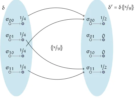
Let us see this on the example we had before:

δ=��

��

x�0

y�0��1�4,� x�0

y�1��1�4,� x�1

y�1��1�4,� x�1 y�0��1�4

��

δ{�y�_x�}=��

��

x�0

y�0��1�2,� x�1 y�1��1�2

��

This is shown in Figure 3.

9_{In other words, it is a real-valued random variable —}_pGCL_{expectations are therefore distributions with the additional}

(11)

σ00

σ01

σ10

σ11 1�₄

1�₄

{�x�_y�}

δ′=δ{�x�_y�} δ

σ00

σ01

σ10

σ11 1�₂

0

[image:11.595.178.415.86.258.2]

1�₂

Figure 3: The assignment in the example.

If we had had the assignmentx∶=4instead ofx∶=y, the result would have been:

δ{�4�_x�}=��

��

x�4

y�0��1�2,� x�4 y�1��1�2

��

3 Programs

Once we have these foundational elements, we can build predicates10 _{that talk about probability}

distributions.

before-distribution predicate

Dp

after-distribution

Dp×Dp→{true,false}

program

Dp

d:P

Aprogram A(δ, δ′) is a particular predicate that links a before-distributionδ, that describes the

situation before running the program (in terms of the probabilities associated with the possible before-states), to anafter-distributionδ′, that describes the situation after running the program (in

terms of the probabilities associated with the possible after-states).

d:P:Img

The program image A(δ)11 is the set of all possible after-distributions δ′ that satisfy the

pro-gramA(δ, δ′).

d:P:Wt

Theprobabilitypof the conditioncbeing satisfied by the program imageA(δ)lies in the set�A(δ)�c��,

where12_:

�A(δ)�c��={�δ′�c�� δ′∈A(δ)}

We refer to this set as theweightof the programAwith respect to the conditionc.

3.1 Program constructs

We define the following program constructs:

d:P:Skip

•skip � δ′=δ

10_{Ordinary logic predicates, featuring all standard logic operators and quantifiers.}

11_{When we have that}_∀_δ

1, δ2●A(δ1)=A(δ2), we may write simplyAinstead ofA(δ).

12_{Note that the operators}_�_{_}_�_and_�_{_}_�_{have been lifted to sets of probability distributions: in both cases the result is a set,}

(12)

d:P:Abrt

•abort � true

d:P:A

•v∶=e � δ′=δ{�e�_v�}

d:P:A:Sng

•vi∶=e � δ′=δ{�e�vi�}

d:P:Seq

•A_;B � ∃δm●A(δ, δm)∧B(δm, δ′)

d:P:Ch:Cnd

•A◁c▷B � ∃δA, δB●A(δ�c�, δA)∧B(δ�¬c�, δB)∧δ′=δA+δB

d:P:Ch:Prb

•A_p⊕B � ∃δA, δB●A�p⋅δ, δA�∧B�(1−p)⋅δ, δB�∧δ′=δA+δB

d:P:Ch:Dmn

•A�B � ∃π, δA, δB●A(δ�π�, δA)∧B(δ�π¯�, δB)∧δ′=δA+δB

d:P:Loop

•c∗A � µX●(A;X)◁c▷skip

The failing programabort is represented by the predicatetrue, which captures the fact that it is maximally unpredictable.

Programskipmakes no changes and immediately terminates. Assignment remaps the distribution as has already been discussed in the previous §2.

Sequential composition is characterised by the existence of a “mid-point” distribution that is the outcome of the first program, and is then fed into the second.

We characterise conditional choice by using the condition (and its negation) to filter the left- and right-hand programs appropriately, and we simply sum the (now effectively disjoint) distributions. Probabilistic choice simply uses the probability and its complement to scale the distributions for merge — this definition preserves all usual properties.

Non-deterministic choice in UTP is obtained by existentially quantifying over all possible weighting distributions, used to weight both sides13_{. In effect the predicate is only satisfied by any}

combina-tion of left and right distribucombina-tions that is pointwise larger than the minimum of both.

The definition of loop that we are proposing is somehow still incomplete, as we still have not provided an ordering relation among programs: we will fix this in the following §4, where we define therefinementrelation between two programs — so in a loop we take the least fixpoint with respect to the ordering introduced by refinement.

d:P:Structure

We can see that all programs that mentionδandδ′can be written as a predicate of the following

shape14_:

∃QuantOf(A)●δ′=BodyOf(A)○δ∧OtherCndOf(A)

where:

• BodyOf(A)is a sequence of modifications (i.e.interleaved restrictions and remapping

opera-tions) that are applied toδin order to obtain the correspondingδ′;

• QuantOf(A)is a list of weighting distributions — all of the quantified probability distributions

can be eliminated via the one-point rule, so thatδ′can be expressed asBodyOf(A)○δ;

• OtherCndOf(A) is a list of any other conditions that are asserted by the program — no

program constructs features other conditions so far, but we will have an extra condition in the generic choice operator, which we will define later on.

In the next subsection we relatepGCLexpectations to this framework; thereafter we discuss some considerations on the topic of choice constructs.

13_{If the weight of one side depends on}_π_{, the weight of the other side will depend on}₍_ι₋_π₎_{, here and later on noted}

as ¯π.

(13)

3.2 Deriving pre-expectations

As an expectation is a random variable (with non-negative real values), that can be represented by a distribution in our framework. Then ifχ′represents a post-expectation andAis a program,

we can define the corresponding pre-expectationχby computing the expected final weight of each

state beforeAis run:

χ(σ)=min�{�χ′⋅δ′� � δ′∈A(ησ)}�

where __⋅_ is the pointwise multiplication of two distribution and we have used the notationησto

represent the distribution null everywhere with the exception of a single stateσmapping to 1: ησ � �†{σ�1}

3.3 More on choice constructs

Choice constructs deserve a bit more attention: we are now going to discuss some of the properties of probabilistic and non-deterministic choice; later on we will define a generic choice construct that covers conditional, probabilistic and non-deterministic choice (and more).

On probabilistic choice

p:P:Ch:Prb:Comm

First of all it is worth noticing that, from the above definition of probabilistic choice, we have the following equivalence:

A_p⊕B≡B₍₁₋_p₎⊕A

p:P:Ch:Prb:Assoc

See proof B.23 Moreover we have the following property:

A_p⊕(B_q⊕C)≡(A_r⊕B)_s⊕C ∧ p=rs ∧ (1−s)=(1−p)(1−q)

A few words on the probabilityp, that parametrises this operator: this may be a number in the

range_[0, 1]in the simplest setting, but in a more general case it is one of the possible values of a

stochastic variablePthat follows a probability distribution, whose probability density functionfP

has the property of being compact in the range_[0, 1]:

�_−∞+∞fP(p)dp=_� 1

0 fP(p)dp=1

The distribution of this stochastic variable does not depend on the program variables, but in an even more general case may depend on other parametersq1, q2, . . . , qn:

�_−∞+∞fPQ(p, q1, q2, . . . , qn)dp=� 1

0 fPQ(p, q1, q2, . . . , qn)dp=fQ(q1, q2, . . . , qn)

On non-deterministic choice

Usually we talk about demonic non-determinism when we are expecting the worst-case behaviour, to model something that behaves as bad as it can for any desired outcome.

Our definition of non-deterministic choiceper sehas no such behaviour, but it will show up with the definition of refinement that we give in §4 or, more in general, whenever we explicitly choose to focus on the worst-case scenario: for this reason we prefer to use the more refer it as to the non-deterministic choice, rather than to the demonic choice.

The non-deterministic choice operator is idempotent according to the above definition: although some definitions in the literature have this property, there are some other where this property does not hold.

(14)

We can reproduce the other behaviour if we run the program twice with probabilistic choice on local variables, and then we merge the outputs by means of a non-deterministic choice: this is a behaviour that has nothing to do with idempotency — we keep the actions of one program separate from the other’s, so we are actually dealing with twodifferentprograms that share the same specification.

On a generic choice construct

d:P:Ch

Another remark that is worth making, is that we can see how all choice constructs look quite similar, or at least they follow a common pattern. The reason is that all choice constructs can be seen as a specific instance of a generic choice construct:

choice�A, B,X� � ∃π, δA, δB●π∈X ∧A(δ�π�, δA)∧B(δ�π¯�, δB)∧δ′=δA+δB

whereX ⊆Dw andDwis the set of all weighting distributions.

In fact we have that:

p:P:Ch:Cnd:Alt

•forX ={ι�c�}we have conditional choice:

A◁c▷B=choice�A, B,{ι�c�}�

p:P:Ch:Prb:Alt

•forX ={p⋅ι}we have probabilistic choice:

A_p⊕B=choice�A, B,{p⋅ι}�

p:P:Ch:Dmn:Alt

•forX =Dwwe have non-deterministic choice:

A�B=choice�A, B,Dw�

p:P:Ch:Or:Alt

Moreover we can see the disjunction of two programs as another kind of choice, whereX ={�, ι}: A∨B=choice�A, B,{�, ι}�

Finally we can also use this generic construct to create new kinds of choices, other than the more traditional ones:

d:P:Ch:CndPrb

• for X = {p⋅ι�c�} we have the conditional probabilistic choice, which behaves like Awith

probabilitypand likeBwith probability(1−p)in the case whencholds, but it behaves likeBifc

does not hold:

A◁_pc▷B=choice�A, B,{p⋅ι�c�}�

p:P:Ch:SwPrb

•forX ={p⋅ι�c�+q⋅ι�¬c�}we have theswitching probabilistic choice, which is equivalent to a

probabilistic choice with parameterpifcholds, with parameterqifcdoes not hold: Ap◁c▷q⊕B=choice�A, B,{p⋅ι�c�+q⋅ι�¬c�}�

d:P:Ch:CndDmn

•forX =Dw�c�we have theconditional non-deterministic choice, which behaves likeA�Bifc

holds, but it behaves likeBifcdoes not hold:

A_c�B=choice�A, B,Dw�c��

p:P:Ch:DmnPrb

•forX ={π � ∀σ●p≤π(σ)≤1−q}, wherep+q≤1, we have thenon-deterministic probabilistic

(15)

p:P:Ch:FDmn

•forX ={p⋅ι � p∈[0..1]}we have thefair non-deterministic choice:

Afair�B=choice�A, B,X ={p⋅ι � p∈[0..1]}�=∃p●A_p⊕B

It is worth noticing that this kind of choice is different from non-deterministic choice (we can view it as a less general form of it), in fact from this definition we have that:

∀δ●(Afair�B)(δ)⊂ (A�B)(δ)

These possibilities have to be explored further, as there can be many more — and potentially more useful than these ones.

A few laws on choice operators

Here is a non-comprehensive list of interesting laws on choice operators, that hold in our frame-work and that can also be found inpGCL:

p:P:Ch:Idem

See proof B.24 Idempotency of choice operators :∀X●choice�A, A,X�≡A

p:P:Ch:Dscrd

See proof B.25 Discarding right-hand option :choice�A, B,{ι}�≡A

p:P:Ch:Dst

See proof B.26 Distributivity of choice operators :

choice�A,(choice�B, C,X2�),X1�≡choice��choice�A, B,X1��,�choice�A, C,X1��,X2�

p:P:Ch:Seq

See proof B.27 Sequential composition :choice�A, B,X�;C≡choice�A_;C, B_;C,X�

p:P:Ch:Flip

See proof B.28 Choice flipping :∀X ●choice�A, B,X�≡choice�B, A,X¯� ∧ X¯ =�π∈Xπ¯

p:P:Ch:Mntn

See proof B.29 Monotonicity of generic choice :_∀δ●X1⊆X2⇒choice�A, B,X1�(δ)⊆choice�A, B,X2�(δ)

4 Refinement

d:P:Rfn

We are going to define the refinement relation between two programs through a relation between the corresponding program images: we say that a programAis refined by a programBwhen for

all conditions and (before-)distributions, the minimal probability that an (after-)distribution from

A(δ)satisfies a condition is less than that forB(δ):

A�B � ∀z, δ●min��A(δ)�z��≤min��B(δ)�z��

Informally, whatever conditionzwe are expecting, programBrefines programAif it is at least “as

good” when it comes to the probability of satisfying it.

The use of min here matches the use inpGCLof it to define demonic choice, so we can see how this notion of refinement creates an order relation that is exactly the one created by the refinement relation used for pGCL. [MM04]

d:P:Rfn:Alt

The whole point of defining refinement this way was to show the similarity with pGCL; moving further and taking advantage of the structure of our framework, we can give an alternative defini-tion:

A�B � ∀δ●B(δ)⊆�A(δ)�△

d:P:RfnSet

where therefinement set_�A(δ)�△is the (up-, convex- and Cauchy-closed) set defined as:

�A(δ)�△ � �δ_△ � δ′≤δ_△≤ι ∧ δ′= � δ′_i∈A(δ�πi�)

(16)

This set includes all after-distributions that are at least as great as those obtainable because of the non-determinism in the behaviour ofA: a program whose image lies in this set for allδ is a

refinement ofA, and hence the term “refinement set”.

From the above definition(s) we can easily demonstrate familiar refinement relations:

A�B � A

A�B � B

A�B � A_p⊕B A�B � A◁c▷B

This comes as no surprise, in fact:

A_p⊕B = ∃π, δA, δB●A(δ�π�, δA)∧B(δ�π¯�, δB)∧δ′=δA+δB ∧ π=p⋅ι A◁c▷B = ∃π, δA, δB●A(δ�π�, δA)∧B(δ�π¯�, δB)∧δ′=δA+δB ∧ π=ι�c�

Concerning disjunction, we have that refinement fails to distinguish it from non-deterministic choice, as their refinement sets are the same:

A�B � A∨B ∧ A∨B � A�B

or, for short,A�B⇔A∨B.

This result is due to the definition we have used for refinement, as we have used the traditional view of non-determinism asdemonicnon-determinism,i.e.that returning the worst possible result for any desired outcome: this is in line with the traditional use of disjunction as a definition for demonic choice.

Alternative definitions of refinement may take advantage of the possibility to distinguish between the operators_�and_∨— this is left for future work.

p:P:Rfn:Ch

See proof B.30 In general, from the definition of refinement and the monotonicity of generic choice, we can show

that:

X2⊆X1 ⇒ choice�A, B,X1��choice�A, B,X2�

p:P:Rfn:Dsj

See proof B.31 It is worth stressing that the reverse implication is false — a counterexample is given by the case

of the disjunction operator, where we have that:

p:P:Rfn:Dsj2

See proof B.32

A∨B � A_p⊕B A∨B � A◁c▷B

4.1 Probabilistic refinement

d:P:PRfn

We want to generalise things even further, and introduce a notion ofprobabilistic refinement:

A�pB � ∀z, δ●p⋅min��A(δ)�z��≤min��B(δ)�z��

We call this ap-accuraterefinement, meaning that the refinement relation�is true in a fractionp

of the possible cases.

d:P:PRfn:Alt

We can give this alternative definition as well, similarly as we did above:

A�pB � ∀δ●B(δ)⊆�p⋅A(δ)�△

wherep⋅A(δ)is the set made of all elements ofA(δ)multiplied byp.

Letp∗ be the highest positive real number such that A p ∗

� B: this is the accuracy with which B

refinesAand is a measure of how “better”Bis when compared toAin any possible case — and

(17)

It is immediate to see that the refinement relation we have defined before is a special case of this more generic operator forp=1,i.e.it is a1-accurate refinement15:

A�B = A�1B

This definition makes it much more meaningful to have a deterministic program on the left-hand side of the refinement relation16_{: the utility of such a thing is for example that a deterministic}

specification can be refined probabilistically by a (potentially) non-deterministic implementation, and the implementation accuracy is a piece of information of great value.

This notion of refinement may seem like generalisation for its own sake, but it has useful real-world applications — an example on medical devices can be found in [SSL10].

5 States and distributions, formally

Now that we have presented the whole idea, let us go down to the details which have been ex-plained informally or in a less general way (when not skipped) in §2.

Examples relative to this part can be found in §A.1.

5.1 States

d:S

A stateσis a total functionσ∶V→W that maps each variableviin the memory to a valuewi.

We useSto note thestate space, which is the set of all possible states. According to this definition we have:

dom₍σ)=V ={v1,v2, . . . ,vn, . . .}

d:S:Alph

We refer to the domain of the state function also as thealphabetof that state: alph₍σ) � dom(σ)

d:T

Wiis thetypeof the variablevi,i.e.vi∶Wi. We note this also as:

type₍vi) � Wi⊂W

whereW is the set containing all types. For now we assume we have only booleans and integers as types.

d:E

Anexpressionon variables is a combination of constants and variables, combined by operators. The set of all expressions isE.

d:E:Ev

An expressionecan be evaluated in a state σby replacing each variablevi it mentions with the

valueσ(vi)that is contained by that variable in that state: doing the calculations with these values

returns theevaluation of the expressioneon the stateσ, which is the value evalσ(e).

Here is a recursive definition, wherekis a constant,F an-ary function andxian expression:

evalσ(k) � k

evalσ(vi) � σ(vi)

evalσ�F(x1, x2, . . . , xn)� � F�evalσ(x1),evalσ(x2), . . . ,evalσ(xn)�

15_{Or a}₁₀₀_{%-accurate refinement, in case we prefer expressing}_p_{as a percentage.}

16_{It is immediate to prove that a deterministic program}_A_{can be refined only by another program}_B_{, which has to be}

(18)

d:E:Ev:SH

As a shorthand notation for the evaluation function, we overload the function state:

σ(e) � evalσ(e)

When an expressionecontains only values and operators, we have that its evaluation is the same

on any state, thus when the notation is clear from the context we will simply writee instead of

evalσ(e)(orσ(e), using the shorthand notation).

p:E:Ev:VS

Using this, we can write that:

σ(e) = evalσ�e{σ(vi)�v_i}� = σ�e{σ(vi)�v_i}� = e{σ(vi)�v_i}

d:S:Sat

Aconditionis a boolean expression: we say that a state satisfies a conditioncwhen it evaluates to

truein that state.

d:A

Anabstract stateα⊆Sis a set of states:

α � {σ1, σ2, . . . , σn, . . .}

d:A:Alph

The alphabet of an abstract state is defined as the set of all the different alphabets that appear in the abstract state:

alph₍α) � {A �A=alph(σ)∧σ∈α}

d:A:LAA

We useSA to note the largest abstract state such that alph(α)={A}:

SA � {σ� alph(σ)=A}

We write it this way as it is the largest subset of S, whose elements are all those states with alphabetA.

d:A:Sat

We say that an abstract state satisfies a conditioncwhen all its elements do.

d:A:Rst

We define therestrictionof an abstract state through a conditioncas a total function _�_�∶(�S×

E)→�S, defined as follows:

α�c� � {σ�σ∈α ∧ σ(c)=true}

p:A:Rst:Alt

See proof B.1 We have that:

α�c�=S�c�∩α

p:A:Rst:T

Clearly if the condition istruewe have:

α�true�=α

p:A:Rst:F

And obviously if the condition isfalse we have:

α�false�=�

5.2 Distributions

d:D

Adistributionχis a partial functionχ∶S�R, that maps some states to real numbers. χ � {σ1�x1, σ2�x2, . . . , σn�xn, . . .}

We refer toxias theweightof that stateσiand we useDto note the set of all possible distributions.

d:D:Wt

The weight of a distributionχis the sum over its domain of all the state weights:

�χ� � � σ∈dom(χ)

(19)

d:D:Wt:Lift

This can be lifted to a setX ⊆D of distributions in an obvious way:

�X� � {�χ� �χ∈X}

d:D:Alph

The alphabet of a distribution is defined as the set of all the different alphabets that appear in the distribution domain:

alph₍χ) � alph�dom(χ)�

d:D:ED

A particular distribution is theempty distribution �α ∶ S � R, which is a distribution such that

img₍�α)={0},i.e.it maps each state in the abstract stateαto0: �α � {σ�0�σ∈α}

d:D:UD

Another particular distribution is theunity distributionια∶S�R, which is a distribution such that

img₍�α)={1},i.e.it maps each state in the abstract stateαto1: ια � {σ�1�σ∈α}

d:D:E:SH / d:D:U:SH

We define the following shorcuts:

�_A � �_S_A ι_A � ι_S_A

�χ � �dom(χ) ιχ � ιdom(χ)

� � � ι � ιS

d:D:Rst

We define therestriction of a distribution through a conditioncas follows: χ�c� � �σ�χ(σ) �σ∈dom(χ)�c��

p:D:Rst:Cnj

From this definition we have:

χ�c1∧c2�=χ�c1��c2�=χ�c2��c1�

Moreover:

p:D:Rst:EqC

See proof B.2 Restriction through equivalent condition :(c1⇔c2) ⇒ χ�c1�=χ�c2�

p:D:Rst:ImC1

See proof B.3 Restriction through implied condition (I) :(c2⇒c1) ⇔ χ�c1��c2�=χ�c1�

p:D:Rst:ImC2

See proof B.4 Restriction through implied condition (II) :(c1⇒¬c2) ⇒ χ�c1��c2�=�

In case we have conditionscσandcα selecting respectively a single stateσand an abstract state α, we simplify the notation as follows:

d:D:RstS

•δ�σ� � δ�cσ�

d:D:RstA

•δ�α� � δ�cα�

d:D:Pnt

We define thepoint distribution(with domainα) as the restriction of a unity distribution to a single

state:

ησ,α � ια�σ�

Concerning the weights of the restricted distributions above we have that:

p:D:Rst:Wt

(20)

p:D:RstS:Wt

•_�δ�σ��=δ(σ)

p:D:RstA:Wt

•�δ�α��=∑_σ_∈_αδ(σ)

p:D:Pnt:Wt

•�ησ,α�=1

d:D:RstD

We also define therestriction of a distribution through another distributionas follows:

χ1�χ2� � �σ�χ1(σ)⋅χ2(σ) �σ∈dom(χ1)∩dom(χ2)�

p:D:RstD:Cmm

From this definition we have:

χ1�χ2�=χ2�χ1�

p:D:Rst:Alt

See proof B.5 The reason why we call these operations in a similar way is that if we can see that the restriction of

a distribution through a condition as a generalization to distributions of the restriction of abstract states through a condition, the restriction of a distribution through a distribution can be seen as a further generalization:

χ�c�=χ�ιχ�c��

All of this can be lifted to a setX ⊆D of distributions in an obvious way:

d:D:Rst:Lift

•X�c�={χ�c� �χ∈X}

d:D:RstD:Lift

•X�χ�={ξ�χ� �ξ∈X}

Operations on distributions

d:D:Sum

Thesumof distributions is defined as:

χ1+χ2 � �σ��χ1(σ)+χ2(σ)��

From this definition we have that:

p:D:Sum:Wt

•_�χ1+χ2�=�χ1�+�χ2�

p:D:Sum:Rst

•(χ1+χ2)�π�=χ1�π�+χ2�π�

p:D:Sum:CS

See proof B.6 Thanks to the latter property we can split a distribution into two other distributions, where all the

elements of one satisy a given conditionc, while the elements of the other do not: χ=χ�c�+χ�¬c�

d:D:Mul

Themultiplication by a scalar numberis defined as:

n⋅χ � �σ��n⋅χ(σ)� �

d:D:Prod

The restriction of a distribution through another distribution may be regarded as a kind of product, and sometimes it is easier to think of it in these terms, so we define theproductof two distribution as:

χ1⋅χ2 � χ1�χ2�

p:D:Prod:Cmm

From this definition we have that:

(21)

Types of distributions

d:D:WD

Aweighting distributionπis a distribution such that img(π)⊆[0..1].

We useDwto note the subset ofD of all weighting distributions.

d:D:WD:Cmp

Given a weigthing distributionπ, we define its complementary weighting distribution ¯πas:

¯

π � ιπ−π

p:D:WD:Rst

See proof B.7 Restriction :π1�π2�∈Dw

d:D:PD

Aprobability distributionδis a weighting distribution such that�δ�≤1: δ � {σ1�p1, σ2�p2, . . . , σn�pn, . . .}

We useDpto note the subset ofDwof all probability distributions.

In this case we will refer to the weightpi as to theprobability17of the stateσi; likewise we will

talk of the probability of an abstract state18_{, rather than of its weight.}

p:D:PD:Rst

See proof B.8 Restriction :δ�π�∈Dp

In the remainder of this document we will be talking mostly of probability distributions, so we will usually be referring to them simply as “distributions”.

Whenever we want to use this term in the more general meaning we have used so far, we will rather use “general distributions”.

6 Assignments

An assignment performed in a stateσis an operationvi∶=ei, that updates the value contained in

viwithσ(ei).

InUTPwe usually use a dash to mark a variable, in order to refer to the new valuevi′it contains:

the same convention is adopted here. Moreover we will use dashes in a similar way to denote after-states(σ′) andafter-distributions(δ′).

d:S:SA

We use the following notation fornsimultaneous assignments of the expressionse1, e2, . . . , ento

the variablesv1,v2, . . .vn∈V:

v∶=e � v1,v2, . . . ,vn∶=e1, e2, . . . , en

where v= � �� v1 v2 ⋮ vn � ��

∈V and e=

� �� e1 e2 ⋮ en � �� ∈E d:E:Ev:VSH

Moreover, we also use the following shorthand notation:

σ(v) �

� ��

σ(v1) σ(v2)

⋮

σ(vn)

� ��

d:S:VMap

By using this notation we can define a vectorial extension for the map operator:

v�w � {vi�wi�1≤i≤n}

17_δ₍_σ₎_{is a function of}_σ_{and is what is usually referred to as the}_{probability mass function}_{: it represents the way the}

probability is distributed depending onσ.

(22)

p:S:Alt

We can use this to give a compact definition of a state:

σ=v�w

where w= � �� w1 w2 ⋮ wn � �� ∈W d:E:Sub

We use the following notation for simultaneous substitutions19_{f1�_g1}{f2�_g2}�{fn�_gn}:

{f�_g} � {f1�_g1}{f2�_g2}�{fn�_gn}

where f= � �� f1 f2 ⋮ fn � ��

and g=

� �� g1 g2 ⋮ gn � �� d:E:Sub2

When the substitution{f�_g}is applied to a vector of expressions_e, the meaning is the following:

e{f�_g} �

� ��

e1{f�g} e2{f�_g}

⋮

en{f�_g}

� ��

d:E:Comp

The composition of two expression vectors f and e is defined as a particular substitution that

involves the variable vectorv:

f○e � f{e�_v}=

� ��

f1{e�v} f2{e�v}

⋮

fn{e�v}

� ��

We can read the notationf○easfaftere.

p:E:Ev:Comp

Concerning the evaluation of this vector we have

σ(f○e)=σ(f{e�_v})=_σ(_f{σ(e)�_v})=_f{σ(e)�_v}

This is equivalent to evaluatingfin a stateζsuch thatζ(v)=σ(e).

Now it should be clear why we intentionally use a symbol like○and the word “after”, which both remind of functional composition: if for every expression and variable vectorseandvwe define

an associated functione_v∶W �W as:

e_v(w)=evalv�w(e) then for any stateσ=v�w, we have thatσ(f○e)=f_v�e_v(w)�:

��

σ(f○e)=f_v(w∗)

w∗=e_v(w)

d:E:Comp:Iter

When composing the same expression fork≥1times, we use the following notation: ek � e○e○ ⋅ ⋅ ⋅ ○e

��

ktimes

We define that fork=0this notation has the following meaning: e0 � v

19_{For this to make sense, it must be the case that}_∀_i_≠_j_●_g

(23)

6.1 The inverse-image set

d:S:Inv

Let us now define theinverse-image setfor a generic assignmentv∶=e, after which the new mapping

of the variable vector is a stateσ′:

Inv(v∶=e, σ′) � �σ�σ′(v)=σ(e) ∧ σ∈Salph(σ′)�

d:A:Inv

We can generalize this to an abstract stateα′:

Inv(v∶=e, α′) � � σ′∈α′

Inv(v∶=e, σ′)

The abstract stateαis the set of all the possible states before the assignment that are compatible

with the result of the new mapping being in the abstract stateα′.

p:A:Inv:Dsj

Due to the fact that the evaluation of an expression is an injective function we have that:

Inv(v∶=e, σ1)∩Inv(v∶=e, σ2)=�⇔σ1≠σ2

p:A:Inv:EqR

Thanks to this property, if the evaluation of an expressioneis defined on all of the states belonging

to an abstract stateα, we have that it is possible to partitionαthroughe.

In fact if we have a relationRedefined as:

σ1Reσ2 ⇔ σ1(e)=σ2(e)

this is an equivalence relation among states belonging to an abstract stateα, that is partitioned

into equivalence classes corresponding to inverse-image setsα′:

α= �

σ′∈α′

Inv(v∶=e, σ′)

where each class is represented by a stateσsuch thatσ(e)=σ′(v).

p:S:Inv:Nest

See proof B.9 Nestedinverse-image set:Inv�v∶=e,Inv(v∶=f,{σ}) �=Inv�v∶=f{e�_v}_,{_σ}�

Examples relative to this subsection can be found in §A.1.

6.2 The remap operator

d:D:Rmp

Theremapoperator is defined as follows:

δ{�e�_v�} � �_σ′��_δ�Inv(v∶=_e,{_σ′})�� alph(_σ′)∈alph(_δ)�

p:D:Rmp:Alt

Which is:

(δ{�e�_v�})(_σ′) � �∑_δ(_σ) � _σ′=_σ†{v�eval_σ(_e)�

p:D:Rmp:Alph

From the definition we can see that after applying the remap operator the alphabet of the resulting distribution is the same as the alphabet of the original distribution:

alph₍δ{�e�_v�})=alph(_δ)

d:D:Rmp:Sng

We overload this notation to account for assignment to a single variable:

δ{�ei�_v_i�} � _δ{�(ei)�_(v_i₎�}

d:D:Rmp:Iter

We define a compact notation for multiple application of the same operation:

δ{�e�_v�}k � _δ{�e�_v�}{�e�_v�}_{. . .}{�e�_v�}

��

(24)

d:D:Dash

A sequence of assignments causes the distribution to evolve and we want to keep track of changes. In fact we have that after an assignmentv ∶=ewhen the distribution isδ, we have an evolution

towards a newδ′.

We can write this as:

δ′=δ{�e�_v�}

Examples relative to this subsection can be found in §A.1.

Properties

p:D:Rmp:Lin

See proof B.10 From the definitions of sum and multiplication, we have that the remap operator is a linear one:

�x⋅δ{�e�_v�}+_y⋅_δ{�f�_v�}�{�g�_v�}=_x⋅_δ{�e�_v�}{�g�_v�}+_y⋅_δ{�f�_v�}{�g�_v�}

Here are some other properties:

p:D:Rmp:Comp1

See proof B.11 Composition (I) :δ{�e�_v�}{�f�_v�}=_δ{�f{e�v}�_v�}

p:D:Rmp:Comp2

See proof B.12 Composition (II) :δ{�e�_v�}{�f�_v�}=_δ{�f○e�_v�}

p:D:Rmp:Comp3

See proof B.13 Composition (III) :δ{�e�_v_i�}{�f�_v_j�}=_δ{�(e,f{e�vi})�(vi,vj)�}

p:D:Rmp:Comp4

See proof B.14 Composition (IV) :δ{�e�_v_i�}{�f�_v_i�}=_δ{�f{e�_v

i}�vi�}

p:D:Rmp:Iter

See proof B.15 Iteration :δ{�e�_v�}k=_δ{�ek

�v�}

p:D:Rmp:Cmm1

See proof B.16 Commutativity (I) :δ{�e�_v_i�}{�f�_v_j�}=_δ{�f{e�_v

i}�vj�}{�e�vi�}iffvj∉fv(e)

p:D:Rmp:Cmm2

See proof B.17 Commutativity (II) :δ{�e�_v_i�}{�f�_v_j�}=_δ{�f�_v_j�}{�e�_v_i�}iffv_i∉fv(_f)∧v_j∉fv(_e)

p:D:Rst:ES

See proof B.18 Expression substitution :δ�f=g�{�e�_v�}=_δ�_f=_g�{�e{f�g}�_v�}

p:D:Rmp:Rst1

See proof B.19 Contradiction :_∀σ∈dom(δ)●σ(c{e�_v})=false ∧ _δ≠_� ⇔ _δ{�e�_v�}�_c�=_�

p:D:Rmp:Rst2

See proof B.20 Assertion :∀σ∈dom(δ)●σ(c{e�_v})=true⇔ _δ{�e�_v�}�_c�=_δ{�e�_v�}

p:D:Rst:Rmp

See proof B.21 Remapping a condition :δ{�e�_v�}�_c�=_δ�_c{e�_v}�{�e�_v�}

p:D:Rmp:Wt

See proof B.22 Weight of a distribution after remapping :�δ{�e�_v�}�=�_δ�iff_σ(_e)is defined in dom(_δ)

7 Conclusion and future work

We have provided an encoding of the semantics of pGCL in UTP, as a homogeneous relation on the alphabet_{δ, δ′}, where the before and after variables are distributions over program states. The

key is that our semantics models probabilistic programs as predicate transformers, so allowing us to claim that “probabilistic programs are predicates too”!

Such programs may feature both demonic and probabilistic choice: this is non-trivial and at the time of this writing there is still no satisfactoryUTPtheory that embeds such a feature —unifying probabilism with other programming constructs in the style of Unifying Theories of Programming is aso-far-unachieved goal, according to the aforementioned talk by Chen and Sanders [CS09] at FM09.

Towards a UTP style framework to deal with probabilities

Towards a

UTP

-style framework

to deal with probabilities

Riccardo Bresciani, Andrew Butterfield

Contents

1 Introduction

1.1

UTP

: general principles

1.2

pGCL

1.3 Probabilistic

UTP

1.4 Other background material

2 States and distributions, informally

3 Programs

3.1 Program constructs

3.2 Deriving pre-expectations

3.3 More on choice constructs

4 Refinement

4.1 Probabilistic refinement

5 States and distributions, formally

5.1 States

5.2 Distributions

6 Assignments

6.1 The inverse-image set

6.2 The remap operator

7 Conclusion and future work