Models for Intersection and Collision with Earth’s Orbit
Eric Sullivan
* *Student, Pittsford Mendon High School Class of 2016
Abstract- Data from the article “Equations for Planetary Ellipses” was used in order to create parametric and polar versions of the planetary equations. Using the standard form for both a parametric ellipse and a polar ellipse these equations were written. With the polar equations, collisions and intersections can be determined. In order to see if intersections or collisions were possible, four standard models of orbital interference were created. These models prove that there are potential for objects to collide with Earth. The derivative of each other the orbital interference models was determined in order to know the rate of change at any point. The most useful point would be an intersection or collision point.
Index Terms- collision, eccentricity, ellipse equations, intersection, parametric equations, planetary orbits, polar equations I. INTRODUCTION
ith the data in the article “Equations for Planetary Ellipses”, the equations given were converted into parametric and polar form. This was decided to be done in order to determine if some other object (such as a large meteor or asteroid) will possibly collide or intersect with Earth’s orbit. The parametric form will not be a useful tool in this case due to the fact that the intersecting or colliding orbits have been treated as parabolas. In parametric form, a quadratic equation has two separate parametric equations. In any case, the parametric equations for the eight planets have been recorded. Four standard models of parabolic equations that can potentially interfere with a planet’s orbit were determined and used to model intersections and collisions. These models are left in raw equation form due to the unknown nature and values given with an intersecting or colliding body. Majority of this experimentation was used in regards to Earth’s orbit.
II. IDENTIFY, RESEARCH AND COLLECT IDEA
The equation for Earth’s orbit came from the article “Equations for Planetary Ellipses”. The standard form for parametric ellipses and polar ellipses were found on an online source. The importance of determining intersection or collision points with Earth’s orbit is so that we know if any object will ever collide with Earth. The models are only in parabolic form because due to the layout of an elliptical orbit, only a part of the orbit will interact with Earth’s orbit. Half of an ellipse will be inactive in collision or intersection with Earth’s orbit. However, it may interact with another planet’s orbit.
III. WRITE DOWN YOUR STUDIES AND FINDINGS
Since all the models are being compared to Earth’s orbit, the value for c equals 2.55. In table 2, the parametric forms for the eight planets orbits are listed. The polar form for the eight planets is in table 3. Table 1 holds the rectangular planetary ellipse equations. Table 4 includes all of the equations designed for Earth. Tables 5 and 6 are the equations for the interference models. Table 5 has the models in rectangular form while Table 6 has them in polar form.
The model standard form was given, it was then re-formatted into the model interference form in order to be converted into polar form more easily. These standard interference forms where then converted into standard polar form in order to test for collision or
intersection. The model form in polar were then set equal to the Earth equation in polar form.
Collision Test: To test for collision, set the two equations equal to each other. If there is an answer then that point is a possible collision. The equations below are number as 1, 2, 3, and 4 respectively.
1.
12𝑎(sec tan 𝜃) + 𝑐(sec 𝜃) ± 1 2√𝑎 cos 𝜃√
1 𝑎(sin 𝜃
2) + 4𝑐(sin cos 𝜃) + 4𝑘(cos 𝜃2) = (150)(149.9783) √(150)2−(2.55)2(cos 𝜃)2
2. −(1
2𝑎(sec tan 𝜃) + 𝑐(sec 𝜃) ± 1 2√𝑎 cos 𝜃√
1 𝑎(sin 𝜃
2) + 4𝑐(sin cos 𝜃) + 4𝑘(cos 𝜃2)) = (150)(149.9783) √(150)2−(2.55)2(cos 𝜃)2
3.
−cos 𝜃±√cos 𝜃2−4𝑎ℎ sin 𝜃2
−2𝑎 sin 𝜃2
=
(150)(149.9783)
4.
cos 𝜃±√cos 𝜃2−4𝑎ℎ sin 𝜃2−2𝑎 sin 𝜃2
=
(150)(149.9783)
√(150)2−(2.55)2(cos 𝜃)2
For this experiment, four sets of c, k and a were chosen for the first two interference equations written in polar form. The work showing an example of either collision or intersection is shown below. The c value does not change in any example.
Equation #1:
Set 1: {𝑎 = 0.0075𝑘 = 6 𝑐 = 2.55 Equation #2:
Set 1: {
𝑎 = 0.075 𝑘 = 6 𝑐 = 2.55
These values were placed into the corresponding model interference form and then set equal to the equation for Earth’s orbit. The system of equations was then solved for theta.
For this experiment, four sets of c, h and a were chosen for the last two interference equations written in polar form. The work showing an example of either collision or intersection is shown below.
Equation #3: Set 1:{𝑎 = 0.075
ℎ = 2 Equation #4: Set 1:{𝑎 = 0.075
ℎ = 2
The same process for solving the examples for equations 1 and 2 was used.
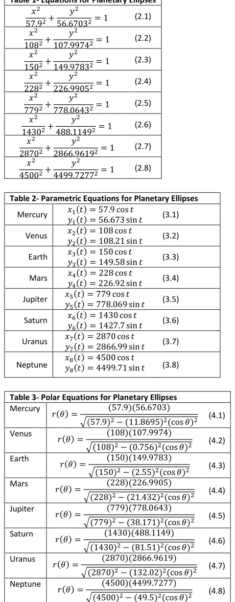
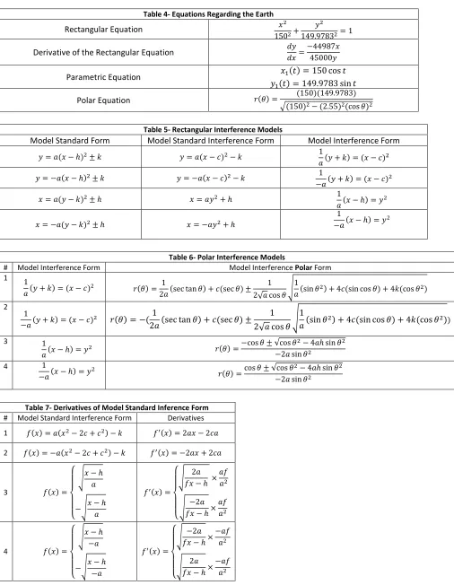
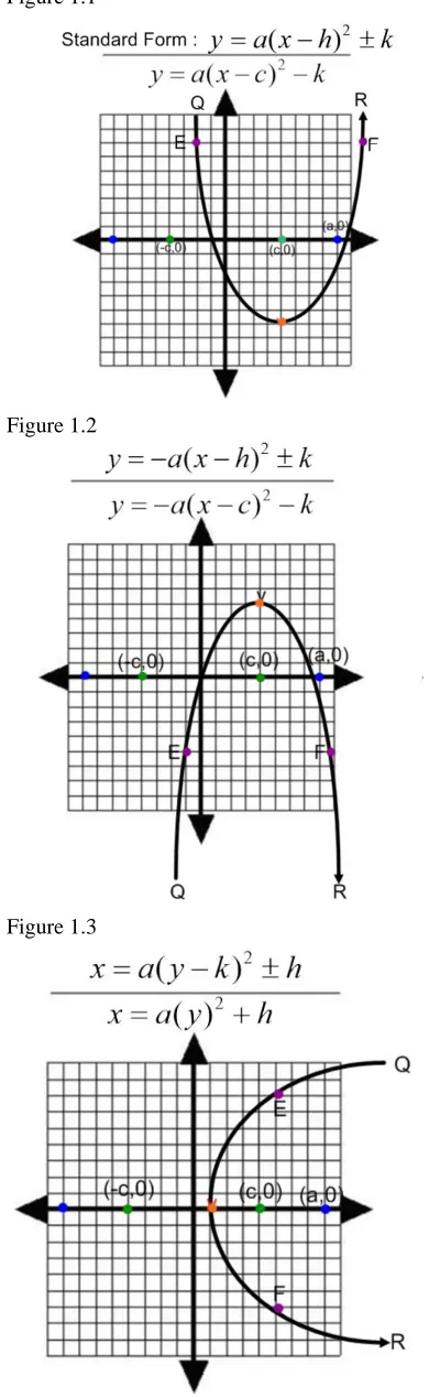
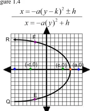
Figure 1.1 represents the first model for interference. In this model, the vertex of the parabolic motion is located at (c,k). In this case the k value is negative and cannot equal a positive value. Figure 1.2 represents the second model for interference. It is similar to the first model, however it is flipped. The vertex still lies at (c,k) but the value for k is positive and cannot equal a negative value. Figure 1.3 is the third model for interference. Unlike the first two, this model has the vertex located along the x axis. Therefore, the vertex for this model is (h,0). In this case, the h values cannot be greater the c. Because of the restriction on positive values and the way this parabolic motion lies, negative h values are possible. Figure 1.4 is the fourth model for interference. Similar to the third model, this parabolic motion has its vertex at (h,0). However, the h values cannot be less then c and negative values cannot exist.
For each model, four interactions are possible. As seen in figures 1.1 through 1.4, the object is always approaching from Q to R. Points E and F are the collision or intersection points. The object can also move from R to Q, the location of the four interactions will change though.
The first interaction as the object moves from Q to R is that there is no collision or intersection. If this is the case, then the two bodies do not interact and thus the motion of both is continuous. The next possible interaction as the object moves from Q to R is that at Point E there is a collision. For this instance Point F does not exist because the two bodies have collided and changed orbits due to the forces involved in the collision. Therefore, both of the equations for the bodies before they collided end at Point E. Another possible
interaction as the object moves from Q to R is that the collision is at Point F and Point E is an intersection. In this case, the objects pass each other at Point E and then later when they reach Point F they collide. Any point after Point F will not exist on the current equation of movement because the forces from the collision will shift the orbital motion of the bodies. The final possible interaction is no collisions at all, instead both Point E and Point F are intersections and the two objects never collide.
The models used only correspond with the axis of symmetry equal to either the x-axis or the y-axis. No vertical intersections or collisions are proposed by this experiment.
The value for the rate of change at any point on either of the interference models is the derivative of those models. The derivative of these models was used to find the slope of the tangent line at any intersection or collision point. The general formulas for the
Table 1- Equations for Planetary Ellipses
𝑥2
57.92+
𝑦2
56.67032= 1 (2.1)
𝑥2
1082+
𝑦2
107.99742= 1 (2.2)
𝑥2
1502+
𝑦2
149.97832= 1 (2.3)
𝑥2
2282+
𝑦2
226.99052= 1 (2.4)
𝑥2
7792+
𝑦2
778.06432= 1 (2.5)
𝑥2
14302+
𝑦2
488.11492= 1 (2.6)
𝑥2
28702+
𝑦2
2866.96192= 1 (2.7)
𝑥2
45002+
𝑦2
4499.72772= 1 (2.8)
Table 2- Parametric Equations for Planetary Ellipses
Mercury 𝑥1(𝑡) = 57.9 cos 𝑡
𝑦1(𝑡) = 56.673 sin 𝑡 (3.1)
Venus 𝑥2(𝑡) = 108 cos 𝑡
𝑦2(𝑡) = 108.21 sin 𝑡 (3.2)
Earth 𝑥𝑦3(𝑡) = 150 cos 𝑡
3(𝑡) = 149.58 sin 𝑡 (3.3) Mars 𝑥4(𝑡) = 228 cos 𝑡
𝑦4(𝑡) = 226.92 sin 𝑡 (3.4)
Jupiter 𝑥5(𝑡) = 779 cos 𝑡
𝑦5(𝑡) = 778.069 sin 𝑡 (3.5)
Saturn 𝑥6(𝑡) = 1430 cos 𝑡
𝑦6(𝑡) = 1427.7 sin 𝑡 (3.6)
Uranus 𝑥7(𝑡) = 2870 cos 𝑡
𝑦7(𝑡) = 2866.99 sin 𝑡 (3.7)
Neptune 𝑥𝑦8(𝑡) = 4500 cos 𝑡
8(𝑡) = 4499.71 sin 𝑡 (3.8)
Table 3- Polar Equations for Planetary Ellipses Mercury
𝑟(𝜃) = (57.9)(56.6703)
√(57.9)2− (11.8695)2(cos 𝜃)2 (4.1) Venus
𝑟(𝜃) = (108)(107.9974)
√(108)2− (0.756)2(cos 𝜃)2 (4.2) Earth
𝑟(𝜃) = (150)(149.9783)
√(150)2− (2.55)2(cos 𝜃)2 (4.3) Mars
𝑟(𝜃) = (228)(226.9905)
√(228)2− (21.432)2(cos 𝜃)2 (4.4) Jupiter
𝑟(𝜃) = (779)(778.0643)
√(779)2− (38.171)2(cos 𝜃)2 (4.5) Saturn
𝑟(𝜃) = (1430)(488.1149)
√(1430)2− (81.51)2(cos 𝜃)2 (4.6) Uranus
𝑟(𝜃) = (2870)(2866.9619)
√(2870)2− (132.02)2(cos 𝜃)2 (4.7) Neptune
𝑟(𝜃) = (4500)(4499.7277)
Table 4- Equations Regarding the Earth
Rectangular Equation 𝑥2
1502+
𝑦2
149.97832= 1
Derivative of the Rectangular Equation 𝑑𝑦
𝑑𝑥=
−44987𝑥 45000𝑦
Parametric Equation 𝑥1(𝑡) = 150 cos 𝑡 𝑦1(𝑡) = 149.9783 sin 𝑡
Polar Equation 𝑟(𝜃) = (150)(149.9783) √(150)2− (2.55)2(cos 𝜃)2
Table 5- Rectangular Interference Models
Model Standard Form Model Standard Interference Form Model Interference Form
𝑦 = 𝑎(𝑥 − ℎ)2± 𝑘 𝑦 = 𝑎(𝑥 − 𝑐)2− 𝑘 1
𝑎(𝑦 + 𝑘) = (𝑥 − 𝑐)
2
𝑦 = −𝑎(𝑥 − ℎ)2± 𝑘 𝑦 = −𝑎(𝑥 − 𝑐)2− 𝑘 1
−𝑎(𝑦 + 𝑘) = (𝑥 − 𝑐)
2
𝑥 = 𝑎(𝑦 − 𝑘)2± ℎ 𝑥 = 𝑎𝑦2+ ℎ 1
𝑎(𝑥 − ℎ) = 𝑦
2
𝑥 = −𝑎(𝑦 − 𝑘)2± ℎ 𝑥 = −𝑎𝑦2+ ℎ
1
−𝑎(𝑥 − ℎ) = 𝑦
2
Table 6- Polar Interference Models
# Model Interference Form Model Interference Polar Form
1 1
𝑎(𝑦 + 𝑘) = (𝑥 − 𝑐)
2 𝑟(𝜃) = 1
2𝑎(sec tan 𝜃) + 𝑐(sec 𝜃) ± 1 2√𝑎 cos 𝜃√
1
𝑎(sin 𝜃2) + 4𝑐(sin cos 𝜃) + 4𝑘(cos 𝜃2)
2
1
−𝑎(𝑦 + 𝑘) = (𝑥 − 𝑐)
2 𝑟(𝜃) = −(1
2𝑎(sec tan 𝜃) + 𝑐(sec 𝜃) ±
1
2√𝑎 cos 𝜃√
1 𝑎(sin 𝜃
2) + 4𝑐(sin cos 𝜃) + 4𝑘(cos 𝜃2))
3 1
𝑎(𝑥 − ℎ) = 𝑦
2 𝑟(𝜃) =−cos 𝜃 ± √cos 𝜃
2− 4𝑎ℎ sin 𝜃2
−2𝑎 sin 𝜃2
4 1
−𝑎(𝑥 − ℎ) = 𝑦
2
𝑟(𝜃) =cos 𝜃 ± √cos 𝜃
2− 4𝑎ℎ sin 𝜃2
−2𝑎 sin 𝜃2
Table 7- Derivatives of Model Standard Inference Form # Model Standard Interference Form Derivatives
1 𝑓(𝑥) = 𝑎(𝑥2− 2𝑐 + 𝑐2) − 𝑘 𝑓′(𝑥) = 2𝑎𝑥 − 2𝑐𝑎
2 𝑓(𝑥) = −𝑎(𝑥2− 2𝑐 + 𝑐2) − 𝑘 𝑓′(𝑥) = −2𝑎𝑥 + 2𝑐𝑎
3 𝑓(𝑥) =
{ √𝑥 − ℎ
𝑎
−√𝑥 − ℎ 𝑎
𝑓′(𝑥) =
{ √ 2𝑎
𝑓𝑥 − ℎ × 𝑎𝑓 𝑎2
√ −2𝑎 𝑓𝑥 − ℎ×
𝑎𝑓 𝑎2
4 𝑓(𝑥) =
{ √𝑥 − ℎ
−𝑎
−√𝑥 − ℎ −𝑎
𝑓′(𝑥) =
{ √ −2𝑎
𝑓𝑥 − ℎ× −𝑎𝑓
𝑎2
√ 2𝑎 𝑓𝑥 − ℎ×
Figure 1.1
Figure 1.2
Figure 1.4
Note: The line between the two equations in all of the figures (figures 1.1, 1.2, 1.3, and 1.4) does not represent division. IV. CONCLUSION
The models provided in this paper give an outline of possible displays and understanding of predicting collisions with Earth. With use of these models, collisions and intersections can be readily predicted. These model interference equations could be used to also find collision or intersection between other planets. The four interaction models (the interference models) used in this report can also be used for the other planets.
ACKNOWLEDGMENT
I would like to acknowledge my math teachers, Mrs. Kimberly Waterbury and Mr. Anthony Martellotta, for their help with sparking my interest in ellipses and how they apply to the planets. I would also like to thank my earth science teacher, Mrs. Sandra Bertrand, for increasing my interest about our solar system and astronomy. My good friend and colleague, Nathan Nabrotzky for his support and help with some of the trickier math.
REFERENCES
Department, The State Education. "Reference Tables for Physical Setting/Earth Science." Reference Tables for Physical Setting/Earth Science. Albany: The University of the State of New York, 2011.
Williams, Dr. David R. NASA Planetary Factsheet. 20 March 2016.
Eric Sullivan - Equations for Planetary Ellipses - published at: "International Journal of Scientific and Research Publications (IJSRP), Volume 6, Issue 5, May 2016 Edition".
AUTHORS
[image:6.612.44.190.61.240.2]