Bottleneck-Based Makespan Algorithm For Cyber Manufacturing System
Salleh Ahmad Bareduan and Sulaiman Hj. Hasan
Faculty of Mechanical and Manufacturing Engineering Universiti Tun Hussein Onn Malaysia (UTHM)
Parit Raja, Batu Pahat, 86400 Johor, Malaysia
Abstract:
This paper presents alternative makespan computation algorithms for cyber manufacturing system (CMS) using bottleneck analysis. The CMS is an Internet-based collaborative design and manufacturing activities between Universiti Tun Hussein Onn Malaysia and the small and medium enterprises. The CMS processes scheduling resembles a four machine flow shop process routing of M1,M2,M3,M4,M3,M4 in which the last three processes of M4,M3,M4 always exhibiting bottleneck characteristics. It was shown that using detail bottleneck characteristic analysis, appropriate alternative bottleneck-based algorithm can be developed to compute the makespan for the CMS scheduling activities. This algorithm shows high accuracy within a specified localised sequence dependent limiting conditions. In cases where the limiting conditions are violated, a bottleneck correction factor is introduced in order to ensure accurate solution. These algorithms can later be used to develop appropriate heuristic to optimise the CMS scheduling problem.
1. Introduction
Flow shop manufacturing is a very common production system found in many manufacturing facilities, assembly lines and industrial processes. It is known that finding an optimal solution for a flow shop scheduling problem is a difficult task [1] and even a basic problem of F3 || Cmax is already
strongly NP-hard [2]. Therefore, many researchers have concentrated their efforts on finding near optimal solution within acceptable computation time using heuristics.
One of the important subclass of flow shop which is quite prominent in industries is re-entrant flow shop. The special feature of a re-entrant flow shop compared to ordinary flow shop is that the
permutation flow shop scheduling problem. Significant works on re-entrant hybrid flow shop were also found in the literature [6, 7, 8] while hybrid techniques which combine lower bound-based algorithm and idle time-based algorithm was reported by Choi and Kim [9].
In scheduling literature, heuristic that utilize the bottleneck approach is known to be among the most successful methods in solving shop scheduling problem. This includes shifting bottleneck heuristic [10, 11] and bottleneck minimal idleness heuristic [12, 13]. However, not much progress is reported on bottleneck approach in solving re-entrant flow shop problem. Among the few researches are Dermirkol and Uzsoy [4] who developed a specific version of shifting bottleneck heuristic to solve the re-entrant flow shop sequence problem.
In this paper we explore and investigated an Internet-based collaborative design and manufacturing process scheduling which resembles a four machine permutation re-entrant flow shop. The study is searching for the potential of developing an effective makespan minimization heuristic by firstly developing makespan computation algorithm using bottleneck analysis. This computation is specifically intended for the cyber manufacturing centre at Universiti Tun Hussein Onn Malaysia (UTHM).
2. Cyber Manufacturing Centre
UTHM has recently developed a cyber manufacturing system (CMS) that allows the university to share the sophisticated and advanced machinery and software available at the university with the small and medium enterprises (SMEs) using Internet technology [14]. The heart of the system is the cyber manufacturing centre (CMC) which consists of an advanced
computer numerical control (CNC) machining centre fully equipped with CMS software that includes computer aided design and computer aided manufacturing (CAD/CAM) system, scheduling system, tool management system and machine monitoring system.
P1 P2 P3 P4 P5 P6 P7
P22 P23
P24 P25
T1
15
T2
3
T3
2
T4
8
T5
2
T6
16 CA D design, virtual
meeting, design review
CA M simulation
Generate CNC program f or prototype
Generate CNC program f or customer Prototype
machining
Parts machining
[image:3.612.112.493.92.185.2]CA D system CA M system CNC postprocessor CNC machine
Figure 1 : Petri Net Model of CMC activities
3. CMC Makespan Computation Under Bottleneck Limitations
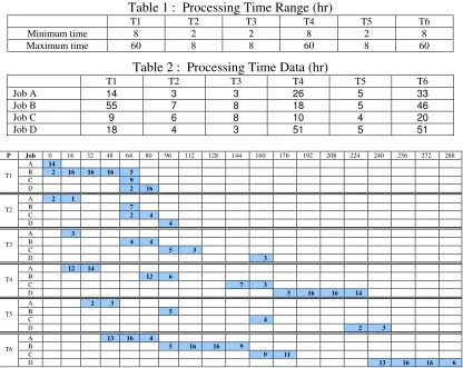
Let say, the CMC is currently having four jobs that need to be processed. Typical processing time ranges for all processes are shown in Table 1. By using the time ranges in Table 1, sets of random data was generated for four jobs that need to be processed. These data is shown in Table 2.
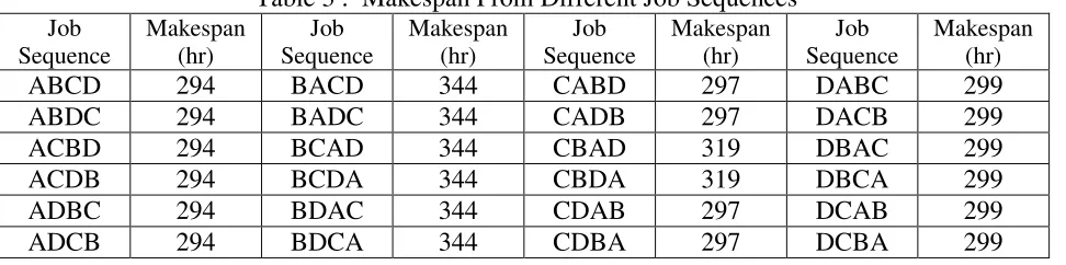
[image:3.612.99.515.351.682.2]Assuming that the data in Table 2 is arranged in the order of First-come-first-served (FCFS), then a Gantt chart representing a FCFS schedule is built as illustrated in Figure 2. The Gantt chart is built by strictly referring to the PN model in Figure 1 together with strict permutation rule.
Table 1 : Processing Time Range (hr)
T1 T2 T3 T4 T5 T6
Minimum time 8 2 2 8 2 8
Maximum time 60 8 8 60 8 60
Table 2 : Processing Time Data (hr)
T1 T2 T3 T4 T5 T6
Job A 14 3 3 26 5 33
Job B 55 7 8 18 5 46
Job C 9 6 8 10 4 20
Job D 18 4 3 51 5 51
P Job 0 16 32 48 64 80 96 112 128 144 160 176 192 208 224 240 256 272 288 A 14
B 2 16 16 16 5
C 9
T1
D 2 16
A 2 1
B 7
C 2 4
T2
D 4
A 3
B 4 4
C 5 3
T3
D 3
A 12 14
B 12 6
C 7 3
T4
D 5 16 16 14
A 2 3
B 5
C 4
T5
D 2 3
A 13 16 4
B 5 16 16 9
C 9 11
T6
D 13 16 16 6
Table 3 : Makespan From Different Job Sequences Job
Sequence
Makespan (hr)
Job Sequence
Makespan (hr)
Job Sequence
Makespan (hr)
Job Sequence
Makespan (hr)
ABCD 294 BACD 344 CABD 297 DABC 299
ABDC 294 BADC 344 CADB 297 DACB 299
ACBD 294 BCAD 344 CBAD 319 DBAC 299
ACDB 294 BCDA 344 CBDA 319 DBCA 299
ADBC 294 BDAC 344 CDAB 297 DCAB 299
ADCB 294 BDCA 344 CDBA 297 DCBA 299
By referring to Table 2, Figure 1 and Figure 2, the scheduling algorithm for the CMC can be written as the followings and is identified as Algorithm 1:
Algorithm 1
Let i = Transition number, process number or work centre number (i=1,2,3,…6) j = Job number (j=1,2,3,…n)
Start (i,j) = start time of the jth job at ith work centre.
Stop (i,j) = stop time of the jth job at ith work centre.
P(i,j) = processing time of the jth job at ith work centre.
For i=1,2,5,6 and j=1,2,3,…n
Start (i,j) = Max [Stop (i,j-1), Stop (i-1,j)] except Start (1,1) = initial starting time
Stop (i,j) = Start (i,j) + P (i,j)
For i =3,4 and j=1,2,3,…n
Start (i,j) = Max [Stop (i,j-1), Stop (i-1,j), Stop (i+2,j-1)]
Stop (i,j) = Start (i,j) + P(i,j)
Algorithm 1 can also be used to compute the makespan of the schedule arrangement by computing all the start and stop time of each work process (WP). The completion time of the last job at the last WP represents the makespan of the schedule. Since there are a total of 4 jobs to be
arranged, this means that there will be 4! different possible schedule arrangements that can be set. The makespan of these 24 different arrangements are computed using Algorithm 1 and the results are recorded in Table 3.
From Table 3, it can be noticed that the job arrangements which begin with Job A produce the smallest makespan. The second, third and last task can be assigned to any other jobs without affecting the makespan value. On the other hand, the job arrangements which begin with Job B produce the largest makespan. Table 3 also indicates that majority of the makespan value are influenced by the assignment of the first task. Almost all scheduling sequence that begins with the same job will result to the same makespan value. The only exception is the scheduling sequence of CBAD and CBDA which produces higher makespan than other sequence that starts with Job C as the first task.
Let i = process sequence of the job at CMC (i=1,2,3,4,5,6)
j = job number according to the scheduling sequence (j=1,2,3…n) P(i,j) = processing time of the jth job at ith
process sequence
For the job sequences of AXXX, BXXX, CXXX (excluding CBXX) and DXXX, the makespan calculation is:
∑
∑∑
= = =
+
3
1 1
6 4
) , ( )
1 , ( i
n
j i
j i P i
P (Equation 1)
From thorough observation at Figure 2, it can be noted that {P(4,j) + P(5,j) + P(6,j)} is always the bottleneck of the scheduling sequence. This is represented by the value of:
∑∑
= =
n
j i
j i P
1 6
4
) ,
( in Equation 1. Since
∑∑
= =
n
j i
j i P
1 6
4
) ,
( will always result to the same
value at any job sequence, then the makespan is directly influenced by {P(1,1) +
P(2,1) + P(3,1)} which is actually the sum
of the first, second and third processing time for the job assigned as the first task.
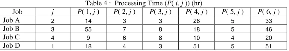
To illustrate the usage of Equation 1, the data in Table 4 is used to compute the makespan for the scheduling sequence of DABC. This scheduling sequence is shown by the sequence arrangement at column j. The makespan computation is:
{P(1,1) + P(2,1) + P(3,1)}
+ {P(4,1) + P(5,1) + P(6,1) + P(4,2) + P(5,2) + P(6,2) + P(4,3) + P(5,3)+ P(6,3) + P(4,4) + P(5,4) + P(6,4)}
= {18 + 4 + 3} + {51 + 5 + 51 + 26 + 5 + 33 + 10 + 4 + 20 + 18 + 5 + 46}
= 299
4. Bottleneck Analysis
Upon computing the makespan value of all 24 possible job sequences using data from Table 2, it is observed that Equation 1 fails to accurately predict the makespan belongs to CBAD and CBDA job sequences. A detail analysis of the Gantt chart representing the job arrangement of CBAD (which belongs to CBXX ) results to the following observation:
{P(1,2) + P(2,2) + P(3,2)}>
{P(2,1) + P(3,1) + P(4,1) + P(5,1) + P(6,1)}
[image:5.612.66.548.611.697.2]This means that with CBAD job sequence, {P(4,1) + P(5,1) + P(6,1)} is not one of the bottleneck of the scheduling arrangement. Since Equation 1 assumes that {P(4,j) + P(5,j) + P(6,j)} are always the bottleneck, therefore this equation is not valid for this job sequence. This is why the makespan for CBAD and CBDA are different from other CXXX. By using the example cases of CBXX and further investigation on all Gantt charts pattern, it was observed that Equation 1 is valid for makespan computation if several localized sequence dependent conditions are met:
Table 4 : Processing Time (P( i, j )) (hr)
Job j P( 1, j ) P( 2, j ) P( 3, j ) P( 4, j ) P( 5, j ) P( 6, j )
Job A 2 14 3 3 26 5 33
Job B 3 55 7 8 18 5 46
Job C 4 9 6 8 10 4 20
(a) For j = 2, {P(2,2) + P(3,2) + VP(2,1)}≤ {P(2,1) + P(3,1) + P(4,1) + P(5,1) + P(6,1)}
or
(, ) (2, 1)
3 2 − +
∑
= j VP j i P i ≤∑
= 6 2 ) 1 , ( i i Pwhere, VP = Virtual Processing Time
(b) For j = 3, {P(2,3) + P(3,3)} + VP(2,1)+ VP(2,2) ≤
{P(2,1) + P(3,1) + P(4,1) + P(5,1) + P(6,1)} + {P(4,2) + P(5,2) + P(6,2)}
or ) 2 , 2 ( ) 1 , 2 ( ) , ( 3 2 − + − +
∑
= j VP j VP j i P i ≤∑
= 6 2 ) 1 , ( i iP +
∑
= − 6 4 ) 1 , ( i j i P
(c) For j = 4, {P(2,4) + P(3,4)} + VP(2,1)+ VP(2,2) + VP(2,3) ≤
{P(2,1) + P(3,1) + P(4,1) + P(5,1) + P(6,1)}+{P(4,2) + P(5,2) + P(6,2)}+ {P(4,3) + P(5,3) + P(6,3)}
or ) 1 , 2 ( ) 2 , 2 ( ) 3 , 2 ( ) , ( 3 2 − + − + − +
∑
= j VP j VP j VP j i P i ≤∑
= 6 2 ) 1 , ( i iP +
∑
= − 6 4 ) 2 , ( i j i
P +
∑
= − 6 4 ) 1 , ( i j i P
(d) P(3,2) ≤ P(6,1), P(3,3) ≤ P(6,2),
P(3,4) ≤ P(6,3)
or ) 1 , 6 ( ) , 3
( j ≤P j−
P for j = 2,3,…n
Virtual processing (VP) time is an imaginary processing time that assumes the starting time of any work process (WP) must begin immediately after the completion of the previous imaginary WP at the same work
centre (WC). For example, consider a job X starting on WC 2 and at the same time a job Y starts at WC 1. If the completion time of job X on WC 2 is earlier than the completion time of job Y at WC 1, under the imaginary concept, the VP of job X at WC 2 is extended from its actual processing time to match the completion time of job Y at WC 1. This means the VP of job X at WC 2 is equivalent to the processing time of job Y at WC 1 since the process at WC 2 for job Y can only be started immediately after the completion of Job Y at WC 1 regardless of the earlier completion time of job X at WC 2. The concept of VP(i,j) is introduced in this condition to simplify the algorithm so that very limited numbers of P(i,j) are shown on the left side of the conditions statement.
The virtual processing time for WC 2 are assigned as the followings:
For j = 1, VP(2,1) = Max [P(2,1), P(1,2)] For j = 2,3…n-1,
VP(2,j) =
∑
∑
∑
− = + = − = − + 1 1 1 2 1 1 ) , 2 ( ) , 1 ( ), , 2 ( ) , 2 ( j k j k j k k VP k P j P k VP Maxcompletion of WP6 of job 2. Condition (c) is to make sure that combination of P1, P 2
and P3 for job 4 is also not a bottleneck for
the schedule. Similarly this will allow WP4 of job 4 to begin immediately after completion of WP6 of job 3. Finally, Condition (d) is to guarantee that P(3,j) will never impose a bottleneck for the scheduling system. Excessive value of P(3,j) may prevent WP4 of any job from beginning immediately after the completion of WP6 of the previous job. If any of the conditions is violated, Equation 1 is no longer valid for the makespan computation. This equation has to be modified and improved in order to absorb the violated conditions.
The general equations that describe all the conditions above can be rewritten as follows:
For j = 2,3,…n P(3, j)≤P(6, j−1)
For j = 2, (, ) (2, 1)
3
2
− +
∑
=j VP j
i P i
≤
∑
=6
2
) 1 , ( i
i P
For j = 3,4,…n
+
∑
∑
−= =
1
1 3
2
) , 2 ( )
, (
j
k i
k VP j
i
P ≤
∑
=6
2
) 1 , ( i
i
P +
∑ ∑
= −
=
6
4 1
2
) , (
i j
k
k i P
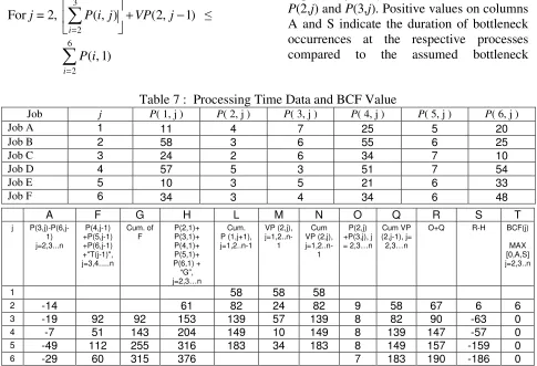
[image:7.612.323.505.86.179.2]Table 7 is specifically developed in order to detect the occurrences of bottleneck at processes other than P(4,j) + P(5,j) + P(6,j) using a set of randomly generated data for 6 job sequence. In other words, this table has the capability to suggest the correction factor need to be added to Equation 1 if the previously described conditions are violated. Column A detects the bottleneck occurrence of P(3,j). This is merely done by comparing the value of P(3,j) with P(6,j-1) for j = 2,3…n. Column S shows the result of investigating the bottleneck occurrence imposed by P(1,j) and its combination with P(2,j) and P(3,j). Positive values on columns A and S indicate the duration of bottleneck occurrences at the respective processes compared to the assumed bottleneck
Table 7 : Processing Time Data and BCF Value
Job j P( 1, j ) P( 2, j ) P( 3, j ) P( 4, j ) P( 5, j ) P( 6, j )
Job A 1 11 4 7 25 5 20
Job B 2 58 3 6 55 6 25
Job C 3 24 2 6 34 7 10
Job D 4 57 5 3 51 7 54
Job E 5 10 3 5 21 6 33
Job F 6 34 3 4 34 6 48
A F G H L M N O Q R S T
j P(3,j)-P(6,j-1) j=2,3...n
P(4,j-1) +P(5,j-1) +P(6,j-1) +"T(j-1)", j=3,4...n
Cum. of F
P(2,1)+ P(3,1)+ P(4,1)+ P(5,1)+ P(6,1) + “G”, j=2,3…n
Cum. P (1,j+1), j=1,2..n-1
VP (2,j),
j=1,2..n-1
Cum VP (2,j),
j=1,2..n-1
P(2,j) +P(3,j), j = 2,3…n
Cum VP (2,j-1), j=
2,3…n
O+Q R-H BCF(j)
MAX [0,A,S] j=2,3..n
1 58 58 58
2 -14 61 82 24 82 9 58 67 6 6
3 -19 92 92 153 139 57 139 8 82 90 -63 0
4 -7 51 143 204 149 10 149 8 139 147 -57 0
5 -49 112 255 316 183 34 183 8 149 157 -159 0
[image:7.612.64.549.382.713.2]duration of P(4,j-1) + P(5,j-1) + P(6,j-1) by Equation 1. Finally, column T determines the actual bottleneck duration among the columns of A and S by selecting the highest positive values. The total value for all jobs at column T represents the bottleneck correction factor (BCF) that must be added to Equation 1 to make it valid for any circumstances. Therefore the corrected version of Equation 1 is:
Makespan =
∑
∑∑
= = =
+ 3
1 1
6
4
) , ( )
1 , ( i
n
j i
j i P i
P +
∑
= nj
j BCF
2
)
( (Equation 2)
where
∑
= nj
j BCF
2
)
( = Summation of BCF
value at column T of Table 7.
For the example shown at Table 7, the makespan for job sequence ABCDEF is:
(11+4+7) +
(25+5+20+55+6+25+34+7+10+51+7+54+2 1+6+33+34+6+48) + (6)
= 475 hours
The makespan of 475 hours is the same with the results from Algorithm 1 for the ABCDEF job sequence in Table 7.
Similarly, the completion time for each job (Cj) can also be computed as the followings:
Cj =
∑
∑∑
= = =
+ 3
1 1
6
4
) , ( )
1 , (
i
j
k i
k i P i
P +
∑
=j
k
k BCF 2
)
( (Equation 3)
For the example shown at Table 7, the completion time of job D (j=4) for job sequence of ABCDEF is:
(11+4+7) +
(25+5+20+55+6+25+34+7+10+51+7+54) + (6)
= 327 hours
To verify the accuracy and reliability of the BCF computation for Equation 2, a total of 10,000 simulations were conducted using random data of between 1 to 80 hours for each of P(1,j), P(2,j), P(3,j), P(4,j),
P(5,j) and P(6,j) with six job sequence for
each simulations. The makespan results from Equation 2 for all the data were compared with ordinary method of makespan computation by determining the earliest start and stop time using Algorithm 1 of each process. The result of the simulation shows that 100% of the makespan values for both methods are the same. This indicates the accuracy and reliability of Equation 2 in computing the makespan of operations scheduling for the CMC.
5. Conclusion
alone, but can also be utilised to describe and develop algorithms for other re-entrant flow shop operation systems that shows significant bottleneck characteristics. With the successful makespan computation using bottleneck analysis, the next phase of this research is to further utilize the bottleneck approach in developing heuristic for optimizing the CMC scheduling sequences.
References
[1] Z. Lian, X. Gu and B. Jiao, A novel particle swarm optimization algorithm for permutation flow-shop scheduling to minimize makespan. Chaos, Solitons and Fractals 2006,
doi:10.1016/j.chaos.2006.05.082 [2] M. Pinedo, Scheduling: Theory, algorithms, and systems. 2nd ed. Upper Saddle River, N.J., Prentice-Hall 2002. [3] S.C. Graves, H.C. Meal, D. Stefek and A.H. Zeghmi. Scheduling of re-entrant flow shops. Journal of Operations Management, 3(4), pp.197-207, 1983
[4] E. Demirkol and R. Uzsoy,
Decomposition methods for reentrant flow shops with sequence dependent setup times, Journal of Scheduling, 3, pp. 115-177, 2000 [5] J.C. Pan and J.S. Chen, Minimizing makespan in re-entrant permutation flow-shops, Journal of Operation Research Society, 54, pp. 642-653, 2003
[6] K. Yura, Cyclic scheduling for re-entrant manufacturing systems, International Journal of Production Economics, 60(61), pp. 523-528, 1999
[7] W.L. Pearn, S.H. Chung, A.Y. Chen and M.H. Yang, A case study on the multistage IC final testing scheduling problem with reentry, International Journal of Production Economics, 88, pp. 257-267, 2004
[8] S.W. Choi SW, Y.D. Kim and G.C. Lee, Minimizing total tardiness of orders with reentrant lots in a hybrid flowshop,
International Journal of Production Research, 43, pp. 2049-2067, 2005 [9] S.W. Choi and Y.D. Kim, Minimizing makespan on an m-machine re-entrant flowshop, Computers & Operations Research 2006,
doi:10.1016/j.cor.2006.09.028
[10] J. Adams, E. Balas and D. Zawack, The shifting bottleneck procedure for job shop scheduling. Management Science, 34, pp. 391-401, 1988
[11] S. Mukherjee and A.K. Chatterjee, Applying machine based decomposition in 2-machine flow shops, European Journal of Operational Research, 169, pp. 723-741, 2006
[12] A.A. Kalir and S.C. Sarin, A near optimal heuristic for the sequencing problem in multiple-batch flow-shops with small equal sublots, Omega, 29, pp. 577-584, 2001 [13] J.B. Wang, F. Shan, B. Jiang and L.Y. Wang. Permutation flow shop scheduling with dominant machines to minimize discounted total weighted completion time, Applied Mathematics and Computation 2006, doi:10.1016/j.amc.2006.04.052
[14] S.A. Bareduan, S.H. Hasan, N.H. Rafai and M.F. Shaari, Cyber manufacturing system for small and medium enterprises: a conceptual framework, Transactions of North American Manufacturing Research Institution for Society of Manufacturing Engineers, 34, pp. 365-372, 2006 [15] G.C. Onwubolu, A flow-shop manufacturing scheduling system with interactive computer graphics, International Journal of Operations & Production