A Mathematical Study of Contaminant Transport with First order Decay and Time dependent Source Concentration in an Aquifer

(1)

A Mathematical Study of Contaminant Transport with

First-order Decay and Time-dependent Source

Concentration in an Aquifer

Rasaq O. Olayiwola

*

_{, Razaq O. Jimoh, Abdulhakeem Yusuf, Samuel Abubakar}

Department of Mathematics and Statistics, Federal University of Technology, PMB 65, Minna, 00176-0000 Nigeria, Niger State, Nigeria *Corresponding Author: [email protected]

Abstract

A mathematical model describing the transport of a conservative contaminant through a homogeneous finite aquifer under transient flow is presented. We assume the aquifer is subjected to contamination due to the time-dependent source concentration. Both the sinusoidally varying and exponentially decreasing forms of seepage velocity are considered for the purposes of studying seasonal variation problems. We use the parameter-expanding method and seek direct eigenfunctions expansion technique to obtain analytical solution of the model. The results are presented graphically and discussed. It is discovered that the contaminant concentration decreases along temporal and spatial directions as initial dispersion coefficient increases and initial groundwater velocity decreases. This concentration decreases as time increases and differs at each point in the domain.

Keywords

Contaminant, First-order Decay,

SeepageVelocity, Aquifer, Advection-dispersionEquation, Parameter-expanding Method

1. Introduction

The intensive size of natural resources and the large production of wastes in modern society often pose a threat to the groundwater quality and already have resultant in many incidents of groundwater contamination. Degradation of groundwater quality can take place over large areas from plane or diffuse sources like deep percolation from intensively farmed fields, or it can be caused by point sources such as septic tank, garbage disposal sites, cemeteries, mine spoils and oil spoils or other accidental entry of pollutants into the underground environment. Another possibility is contamination by line sources of poor quality water, like seepage from polluted streams or intrusion of salt water, from oceans [1,2].

The contaminants in aquifer systems migrate with ground

water flow, any factors that may affect groundwater flow are also likely to influence the migration of contaminants in aquifers. Because contaminants are chemicals or bacteria or virus which are mostly physically, chemically and biologically active, the transport of contaminants are subject to physical, chemical and biological activities, such as contaminant density, adsorption and desorption, retardation, degradation and chemical-biological reactions. Contaminant (solute) transport through a medium is described by a partial differential equation of parabolic type and it is usually known as advection-dispersion equation [3].

Some analytical solutions of the advection-dispersion equation have been proposed in literature with the aim of studying the mechanism of contaminant transport, the movements of pollutants in groundwater and to estimate chemical-physical parameters. Elder [4] by using Taylor's approach and assuming a logarithmic velocity distribution, derived an expression for the longitudinal dispersion coefficient for an infinitely wide open channel. Fischer [5] derived another expression for longitudinal dispersion coefficient assuming that the velocity distribution in lateral direction was the primary mechanism responsible for longitudinal dispersion. Marino [6], van Genucheten [7] and Yadav et al. [8] considered dispersion along unsteady flow. Al-Niami and Rushton [1] considered uniform flow whereas Kumar [9] took unsteady flow against the dispersion in finite porous media.

In the more recent literatures, for one-dimensional problems, analytical solutions have been obtained for varying velocity and dispersivity functions. Among them are solutions to the convection-dispersion equation with: (i) velocity and dispersion coefficient varying in space by Serrano [10]; (ii) velocity varying as a function of cell concentration in an aquifer by Taylor and Jaffe [11]; and (iii) constant velocity but an exponential dispersivity function by Yates [12]. Jaiswal et al. [13] and Kumar et al. [14] obtained analytical solutions for temporally and spatially dependent solute dispersion in one-dimensional semi-infinite media.

(2)

solution for prediction of concentration distribution in an aquifer. Porous domain is considered homogeneous, isotropic, finite and non-reactive. Seepage velocity is a function of time. Time-dependent source concentration is considered at origin. Initially the domain is not solute free. Dispersion is proportional to seepage velocity. First order decay term which is proportional to dispersion coefficient and retardation factor are also considered. To simulate the flow analytically using Eigenfunction Expansion technique, we assume there is no solute flux at end of boundary.

2. Materials and Methods

2.1. Model Formulation

We consider the transport of a contaminant through a homogeneous finite aquifer of length

L

under transient-state flow. It is assumed that initially (i.e., at time

0 t

=

), the aquifer is not clean (i.e., the domain is not solute free). Let

c

_i be the initial contaminant concentration in the aquifer describe the distribution of the concentration at all points of the flow domain. The time-dependent source concentration is assumed at the origin (i.e.,

x

=

0

) of the aquifer. At the end of boundary (i.e.,

x L

=

), we assumed there is no solute flux. Let

c x t

( )

,

be the contaminant concentration in the aquifer at position

x

and time

t

,

( )

,

u x t

the velocity of the medium transporting the contaminants, and

D x t

( )

,

the solute dispersion parameter, if it is independent of position and time, is called dispersion coefficient. Then the problem with first order decay can be mathematically formulated as follows:

( )

,

( )

,

c

R

D x t

u x t c

R c

t

x

σ

∂

₌

∂



∂

₋



₋





∂

_

∂

_

(1)

( )

,

0

( )

,

u x t

=

u f x t

(2) where

R

the retardation factor, which isdefined as

1

d d

k

R

n

ρ

= +

(3)

d

k

is distribution coefficient which is defined as ratio of the adsorbed contaminant concentration to the dissolved contaminants,

ρ

_d is dry unit weight of soil,

n

is porosity,

σ

is first-order decay term or first-order chemical transformation term,

u

₀ is the initial velocity of the medium transporting the contaminants at distance

x

. Here, we made following assumptions:

1. Fluid is of constant density and viscosity.

2. Solute is subject to first-order chemical transformation (i.e.,

σ

≠

0

) and

σ

is a function of space and time.

3. No adsorption,

k

_d

=

0

.

Based on the above assumptions, (1) reduces to

( )

,

( )

,

( )

,

c

_{D x t}

c

_{u x t c}

_{x t c}

t

x

σ

∂

₌

∂



∂

₋



₋





∂



∂



(4)

As initial and boundary conditions, we choose

( )

0

(

( )

)

,

;

0,

0 ,

1 exp

;

0,

0 0;

,

0

i

c x t

c

x

t

c x t

c

qt

x

t

c

_{x L}

_t

x





=

≥

=



=

+

−

=

_{> }



∂

₌

_≥

_



∂



, (5)

where

c

_i is the initial contaminant concentration in the aquifer,

c

₀ is the solute concentration and

q

is the parameter like flow resistance coefficient.

2.2. Method of Solution

Ebach and White [15], have established that the dispersion coefficient vary approximately directly to flow velocity, for different types of porous medium. Here, we let

( )

,

( )

,

D x t

=

au x t

in (4), where

a

is the dispersivity that depends upon the pore geometry. Also, first order decay term which is proportional to dispersion coefficient and retardation factor is considered. Using (2), we get

( )

,

0

( )

,

D x t

=

D f x t

(6)

( )

x t

,

0

f x t

( )

,

σ

=

σ

, (7)

where

D

₀

=

au

₀ is an initial dispersion coefficient and

0

aD

0

σ

=

is the first order decay constant.

Using (6) and (7) and combining equations (2) and (4), we obtain

( )

0 , 0 , 0 ,

c _{D f x t} c _{u f x t c} _{f x t c}

t x x

σ

∂ ₌ ∂  ∂ ₋ ₋

 

∂ ∂  ∂ 

(8) Consider the temporally dependent forms of solute dispersion. Let

f x t

( ) ( )

,

=

v t

,

v t

( )

is the seepage velocity. Then, (8) becomes

( )

2

0 2 0 0

1 c

_D

c

_u

c

_c

v t t

x

σ

∂

₌

∂

₋

∂

₋

∂

(9)

(3)

( )

exp

(

)

,

1 v t

=

−

mt

<

, where

m

is the flow resistance coefficient. We introduce a new time variable [16]:

( )

0

t

v s ds

τ

=

∫

(10)

such that

( )

d

_{v t}

dt

τ

₌

and

( )

1 dt

d

τ

=

v t

(11)

Then, (9) and the corresponding initial and boundary conditions (5) become

2

0 2 0 0

c

_D

c

_u

c

_c

x

σ

τ

∂

=

−

∂

(12)

( )

0

(

)

,

;

0,

0 ,

2 ;

0,

0 0;

,

0

i

c x

c

x

c x

c

q

x

c

_{x L}

x

τ





=

≥

=



=

−

=

_{> }



∂

₌

_≥

_

∂



(13)

2.2.1. Non-dimensionalisation

We non-dimensionalised (12) and (13) using the following set of dimensionless variables:

0 2 0 2 2 0 0 0 0

0 0 0

,

D

x

c

x

c

L

c

L

u L

qL

L

u

q

D

τ

σ

′

=

′

=

′

=

′

=

′

=

′

=

(14)

to obtain (after dropping prime)

2

0 0

2

c

_u

c

_c

x

σ

τ

∂

₌

∂

₋

∂

₋

∂

(15)

( )

( ) (

0

)

,

;

0,

0 ,

2 ;

0,

0 0;

1,

0

i

c

c x

x

c

c x

q

x

c

_x

x

τ



=

≥

_{= }



=

−

=

_{> }



∂

₌

_≥

_

∂

_

(16)

For both the expressions of

v t

( )

, the non-dimensional time variable

τ

may be written as:

( )

0

2 ₀ t

D

_{v s ds}

L

τ

=

_∫

(17)

So that for

1. A sinusoidal varying form,

(

)

(

)

0

2

1 cos

D mt

mt

mL

τ

=

− −

(18)

2. An exponentially decreasing form,

(

)

(

)

0

2

1 exp

D

_mt

mL

τ

=

−

,

mt

<

1

(19)

2.2.2. Solution by Parameter-expanding Method

Suppose the solution

c x

( )

,

τ

and the constant

u

₀ in (15) can be expressed as

( )

x

,

c

0

( )

x

,

0

c

1

( )

x

,

02

c

2

( )

x

,

h

.

o

.

t

,

c

τ

=

τ

+

σ

τ

+

σ

τ

+

(20)

2

0 0 0 0 1

. . .

u

=

σ

p

+

σ

p h o t

+

, (21) where

h o t

. . .

read “higher order terms in

σ

₀ . In our analysis we are interested only in the first two terms.

Substituting (20) and (21) into (15) and (16), and processing, we obtain:

2 0 0 2

c

t

x

∂

=

∂

(22)

( )

( ) (

)

0

0 0

1 0

,0

i

,

0,

2 ,

0

x

c

c x

c

q

c

τ

x

=

∂

=

−

=

∂

2 0 1 1 0 0 2

c

_p

_c

t

x

∂

₌

∂

₋

∂

(23)

( )

1

1 1

1

,0

0,

0

x

c

c x

c

x

τ

=

∂

=

∂

Transform (22) to an inhomogeneous equation with homogeneous boundary conditions and seek a direct eigenfunctions expansion, we obtain

( )

(

)

(

)

2 2 2 2 0 2 1 2 0 2 1 1 ₂ 3 ₃

,

2

4

2 2 1

_{2 1}

sin

2 16 1

2 1

n i n n

c x

q

(4)

( )

(

)

(

)

2 2 2 2

0 2 1

2 2

0 ₂

1 3 3

1 1 0 ₂ 2 1 2 2 2 2 7 ₇ 4 4 2 2 ₁ , . 2 1 2 1 sin 2 1 4 2 1 64 2 2 1 ₁ 2 1 n i n n n p c

c n e

c x

n

n _x

p

n

q n _e

n π τ π τ τ π τ π π π τ π π −   −_ _ ∞ ∞ = = −   −_ _ +    _ _   _ ₋_     ₋          = − −   ₋     −   +  _ _   _ ₋_ _ −  _  _ _  __ _ _  _ _ _ _    __₊ _ _ −

∑∑

(

)

2 2 1 1 2 2 2 1 2 2 2 1 5 5 . 2 1 sin 2 1 2 1 2 2 64 2 1 2 _. 2 1 2 1 sin 2 n n n n n _x n e q n _q n n _x π τ π π π τ π π ∞ ∞ = = −   −_ _ ∞ = −         −   −    _ _ _ _{ −}    _ _    _₊ __ _    _ ₋ _  + __ _ _     − −      

∑∑

∑

, (25) where 0 0 0

_σ

u

p

=

.

For the sinusoidally varying velocity, we substitute (18) into (24) and (25) while for the exponentially decreasing velocity, we substitute (19) into (24) and (25).

The computations were done using computer symbolic algebraic package MAPLE.

2.3. Results and Discussion

Analytical solutions given by (24) and (25) are computed for the values of

c

_i

=

200,

c

₀

=

1.0,

L

=

1 ,

km

(

)

0

1, 2, 4

/

,

u

=

km day

₍

2

₎

0 1.5, 3.0, 4.5 / ,

D = km day

(

)

0.2 /

,

q

=

day

m

=

2 /

(

day

)

(for sinusoidally varying velocity) and

m

=

0.9 /

(

day

)

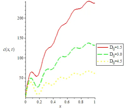
(for exponentially decreasing velocity). The concentration values are depicted graphically in Figures 1 – 16.

The contaminant concentration distribution behaviors along transient groundwater flow for sinusoidally varying velocity are shown in Figures 1 – 8. Figure 1 depicts the graph of

c x t

( )

,

against

x

and

t

for different values of

0

D

. It is observed that the contaminant concentration decreases along temporal and spatial directions as initial

[image:4.595.114.541.72.472.2] [image:4.595.61.291.79.453.2]

dispersion coefficient increases. Figure 2 depicts the graph of

c x t

( )

,

against

x

D

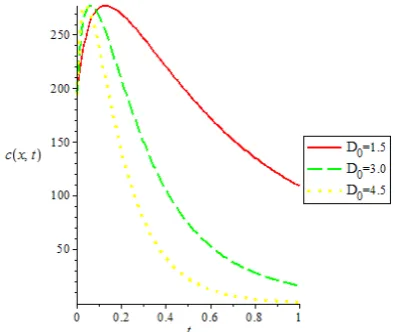
₀. It is observed that the contaminant concentration decreases along spatial direction as initial dispersion coefficient increases. Figure 3 depicts the graph of

c x t

( )

,

against

t

D

₀. It is observed that the contaminant concentration increases and on reaching maximum start decreases along temporal direction as initial dispersion coefficient increases.

Figure 1. Plots of c(x,t) against x and t for different values of D0 and Ci =

[image:4.595.342.514.212.376.2]

200,C0 = 1.0,q = 0.2 , m = 2 U0 = 1, σ0 = 0.004

Figure 2. Plots of c(x,t) against x and t for different values of D0 and Ci =

200,C0 = 1.0,q = 0.2 , m = 2 U0 = 1, σ0 = 0.004 , t = 1

Figure 4 depicts the graph of

c x t

( )

,

against

x

and

t

u

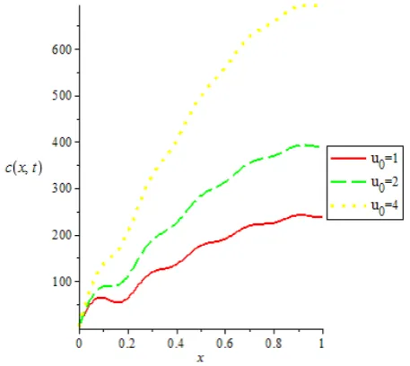
₀ . It is observed that the contaminant concentration increases along temporal and spatial directions as initial groundwater velocity increases. Figure 5 depicts the graph of

c x t

( )

,

against

x

u

₀. It is observed that the contaminant concentration increases along spatial direction as initial groundwater velocity increases. Figure 6 depicts the graph of

( )

,

[image:4.595.332.533.410.582.2]

(5)

[image:5.595.328.542.76.269.2]

Figure 3. Plots of c(x,t) against t for different values of D0 and Ci =

[image:5.595.65.296.81.287.2]

200,C0 = 1.0,q = 0.2 , m = 2 U0 = 1, σ0 = 0.004

Figure 4. Plots of c(x,t) against x and t for different values of U 0 and Ci

= 200,C0 = 1.0,q = 0.2 , m = 2 U0 = 1.5, σ0 = 0.004

= 200,C0 = 1.0,q = 0.2 , m = 2 U0 = 1.5, σ0 = 0.004 , t = 1

[image:5.595.83.283.329.483.2]

= 200,C0 = 1.0,q = 0.2 , m = 2 U0 = 1.5, σ0 = 0.004 , x = 1

c x t

( )

,

against

x

t

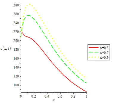
. It is observed that the contaminant concentration decreases along spatial direction as time increases. Figure 8 depicts the graph of

c x t

( )

,

against

t

x

. It is observed that the contaminant concentration increases along temporal direction as position increases.

Figure 7. Plots of c(x,t) against x and t for different values of t and Ci

= 200,C0 = 1.0,q = 0.2 , m = 2 U0 = 1.5, σ0 = 0.004 U0 = 1

[image:5.595.331.540.400.584.2] [image:5.595.65.294.520.724.2]

(6)

[image:6.595.334.532.77.243.2]

of

c x t

( )

,

against

t

D

₀. It is observed that the contaminant concentration increases and on reaching maximum start decreases along temporal direction as initial dispersion coefficient increases.

Figure 8. Plots of c(x,t) against x and t for different values of x and Ci =

[image:6.595.75.286.125.312.2]

200,C0 = 1.0,q = 0.2 , m = 2 U0 = 1.5, σ0 = 0.004 U0 = 1

Figure 9. Plots of c(x,t) against x and t for different values of D0and Ci =

200,C0 = 1.0,q = 0.2 , m = 2 U0 = 1.5, σ0 = 0.004

Figure 10. Plots of c(x,t) against x and t for different values of D0 and Ci

= 200,C0 = 1.0,q = 0.2 , m = 2 U0 = 1.5, σ0 = 0.004 t = 1

Figure 11. Plots of c(x,t) against x and t for different values of D0 and Ci

= 200,C0 = 1.0,q = 0.2 , m = 2 U0 = 1.5, σ0 = 0.004 x = 1

c x t

( )

,

against

x

and

t

u

₀ . It is observed that the contaminant concentration increases along temporal and spatial directions as initial groundwater velocity increases. Figure 13 depicts the graph of

c x t

( )

,

against

x

u

₀. It is observed that the contaminant concentration increases along spatial direction as initial groundwater velocity increases. Figure 14 depicts the graph of

c x t

( )

,

against

t

u

₀. It is observed that the contaminant concentration increases along temporal direction as initial groundwater velocity increases.

Figure 12. Plots of c(x,t) against x and t for different values of U0 and Ci

= 200,C0 = 1.0,q = 0.2 , m = 2 U0 = 1.5, σ0 = 0.004

[image:6.595.91.261.354.509.2] [image:6.595.351.509.419.532.2] [image:6.595.92.272.557.712.2] [image:6.595.335.533.570.729.2]

(7)

c x t

( )

,

against

x

t

. It is observed that the contaminant concentration decreases along spatial direction as time increases. Figure 16 depicts the graph of

c x t

( )

,

against

t

x

. It is observed that the contaminant concentration increases along temporal direction as position increases.

= 200,C0 = 1.0,q = 0.2 , m = 2 U0 = 1.5, σ0 = 0.004 x = 1

Figure 15. Plots of c(x,t) against x and t for different values of t and

Ci = 200,C0 = 1.0,q = 0.2 , m = 2 U0 = 1.5, σ0 = 0.004 U0 = 1

Figure 16. Plots of c(x,t) against x and t for different values of x and Ci

= 200,C0 = 1.0,q = 0.2 , m = 2 U0 = 1.5, σ0 = 0.004 U0 = 1

It is worth pointing out that the effect observed in Figures 7 and 15, is an indication that as time increases in an aquifer, contaminant concentration decreases. Also, the effect of observed in Figures 8 and 16, is an indication that at each point in an aquifer, contaminant concentration defers.

3. Conclusion

A solute transport model with time dependent source concentration formulated to predict contaminant concentration along transient groundwater flow in a homogeneous finite aquifer is solved analytically using parameter expanding method and direct eigenfunctions expansion technique. The governing parameters of the problem are the initial dispersion coefficient (

D

₀) and initial groundwater velocity (

u

₀). Our results showed that the contaminant concentration decreases along temporal and spatial directions as initial dispersion coefficient increases and initial groundwater velocity decreases. This concentration decreases as time increases and differs at each point in the domain.

REFERENCES

[1] N. S. Al-Niami and K. R. Rushtom. Analysis of flow against dispersion in porous media, Journal of Hydrology, Vol.33, No.1-2, 87-97, 1977.

[2] U. Y. Shamir and D. R. F. Harleman. Dispersion in layered porous media, Journal of Hydraulics Division, Vol.95, No.7, 237-260, 1967.

[3] D. K. Jaiswal and A. Kumar. Analytical solution of advection-dispersion equation for varying pulse type input point source in one-dimension, International Journal of Eng. Sci. and Techn. Vol.3, No.1, 22–29, 2011.

[4] J. W. Elder. The dispersion of marked fluid in turbulent shear flow, J. Fluid Mech,. Vol.5, 544-560, 1959.

[5] H. B. Fischer. The mechanics of dispersion in natural streams, J. Hydraul. Div. ASCE, Vol.93, No.6, 187-216, 1967. [6] M. A. Marino. Disrtibution of contaminants in porous media

flow, Water Resour. Res., Vol.10, No.5, 1013-1018, 1974. [7] M. Th. Van Genuchten. Analytical Solutions for chemical

transport with Simultaneous adsorption, zero-order production and first order decay, J. of Hydrology, Vol.49, No.3-4, 213-233, 1981.

[8] R. R. Yadava, R. R. Vinda, and N. Kumar. One–dimensional dispersion in unsteady flow in an adsorbing porous medium: An analytical solution, Hydrological Processes, Vol.4, No.2, 189–196, 1990.

[9] N. Kumar. Dispersion of pollutants in semi-infinite porous media with unsteady velocity distribution, Nordic Hydrology, Vol.14, No.3, 167-178, 1983.

[image:7.595.80.278.165.332.2] [image:7.595.87.515.367.749.2] [image:7.595.86.283.553.726.2]

(8)

recharge and variable velocity, and its analytical solution, Water Resour. Res. Vol.28, No.7, 1801–1808, 1992.

[11] S. W. Taylor, and P. R. Jaffe. Enhanced in-situ biodegradation and aquifer Permeability reduction, J. Environ. Eng., Vol.117, 24–25, 1991.

[12] S. R. Yates. An analytical solution for one- dimensional transport in porous media with an exponential dispersion function, Water Resour. Res., Vol.28, No.8, 2149–2153, 1992.

[13] D. K. Jaiswal, A. Kumar, N. Kumar and R. R. Yadava. Analytical solutions for temporally and spatially dependent solute dispersion of pulse type input concentration in one dimensional semi-infinite media, Journal of Hydro-

environment Research, Vol.2, 254–263, 2009.

[14] A. Kumar, D.K. Jaiswal and N. Kumar. Analytical solutions to one-dimensional advection-diffusion with variable coefficients in semi-infinite media, Journal of Hydrology, Vol.380, No.3-4, 330-337, 2010.

[15] E. H. Ebach and R. White. Mixing of fluids flowing through beds of packed soils, J. of Amer. Inst. Chem. Eng., Vol.4, 161-164, 1958.