On HPM Approximations for the Cumulative Normal
Distribution Function
V. K. Shchigolev
DepartmentofTheoreticalPhysics,UlyanovskStateUniversity,Ulyanovsk,432000,RussianFederation
Copyright c2019 by authors, all rights reserved. Authors agree that this article remains permanently open access under the terms of the Creative Commons Attribution License 4.0 International License
Abstract
In this paper, some new approximations to the cumulative distribution function of the standard normal distribution via the He’s homotopy perturbation method are proposed. There are several methods which provide an approximation of the integral in the formula for the cumulative distribution function by different numerical methods. For the same purpose, we first establish a differential equation of the second order that the cumulative distribution function satisfied subjected with the certain initial conditions. Then we apply the Homotopy Perturbation Method to solve the Cauchy problem for the governing equation. As well known, the result of solving an equation by this method and the convergence rate greatly depend on the choice of homotopy applied. Therefore, we consider two cases in this work. In one case, we construct the homotopy from the idea of simplicity. In the next case, we just follow the procedure of the general approach proposed early. As a result, we obtain several approximations which can be are easily calculated and are better than some other approximations. Numerical comparison shows that our approximations are very accurate.Keywords
Normal Distribution, Cumulative Distribution Function, Approximations, Homotopy Perturbation Method1
Introduction
The importance of the normal distribution in many areas of science (for example, in mathematical statistics and statistical physics) follows from the central limit theorem of probabil-ity theory. If the observation result is the sum of many random weakly interdependent quantities, each of which makes a small contribution relative to the total sum, then with an increase in the number of terms, the distribution of the centered and nor-malized result tends to normal. This law of probability the-ory has the consequence of a wide distribution of the normal distribution, which was one of the reasons for its name. The normal distribution [1], also called the Gauss or Gauss Laplace distribution, is the probability distribution, which in the one-dimensional case is given by a probability density function that
coincides with the Gauss function:
f(x) = 1
σ√2π e
−(x−µ) 2
2σ2 , (1)
where the parameterµis the mean or mathematical expecta-tion of the distribuexpecta-tion, the median and the mode of distribu-tion, and the parameterσis the standard deviation (σ2 is the dispersion or the variance) of the distribution. Thus, the one-dimensional normal distribution is a two-parameter family of distributions. The standard normal distribution is called the normal distribution with the expectationµ = 0and the stan-dard deviationσ= 1.
If a random variable x is normally distributed with zero mean and the standard deviation, then its probability density function (1) is,
f(x) = √1
2π e
−x 2
2 . (2)
A wide usage of this distribution is due to the fact that it is an infinitely divisible continuous distribution with finite vari-ance. Therefore, some others distributions, for example, the binomial and Poisson ones, approach it in the limit. Moreover, many non-deterministic physical processes are modeled by this distribution. The cumulative distribution function (CDF) of the standard normal distribution is the integral
Φ(x) = √1
2π
x
Z
−∞
e−t
2
2 dt. (3)
Unfortunately,Φ(x)cannot be expressed in a closed form in terms of elementary functions for all values ofxwhich would be useful for the practical needs, many numerical approxima-tions forΦ(x)are known. A number of approximate functions for CDF have been proposed (see, for example, [2, 3], and ref-erences therein). Let us represent CDF (3) in the following form
Φ(x) =1 2 +
1
√
2π
x
Z
0
e− t2
2dt. (4)
can be expressed by means of the error function erf(x) = 2
√
π x
R
0
e−t2dtas
Φ(x) = 1 2
1 +erf
x
√
2
. (5)
Therefore, the problem of approximatingΦ(x)is equivalent to the problem of approximating the error function. There are sev-eral methods (see, for example, [4]) which provide an approx-imation of the integral by different numerical methods: Taylor series, asymptotic series, continual fractions, and some others. For more, several other papers should be mentioned where dif-ferent approximate formulae were obtained forΦ(x), such as [5]-[10].
It could be mentioned that in [4] the application of the homo-topy perturbation method (HPM) to calculate an approximate analytical solution of the normal distribution integral was pro-posed. Besides, after solving the Gaussian integral by HPM, the result could serve as the base to solve other integrals like error function and the cumulative distribution function. The basic idea of [4] is that the integral similar to (4) can be refor-mulated as a differential equation subjected to a certain initial condition. Being applied to equation (4), this means that it is necessary to solve
Φ0(x)−√1
2π e
−x2
2 = 0 (6)
with the initial conditionΦ(0) = 1
2 that follows directly from
(4). As noted in [4], the solution for (6) is similar, qualita-tively, to a hyperbolic tangent because whenxtends to±∞, the derivativeΦ0(x)tends to zero, hence by symmetry,Φ(x)
tends to the same constant on both directions. It is why the authors of [4] made the conclusion that the first approach of the HPM method contains a hyperbolic term. Then they estab-lished a differential equation that may be solved using hyper-bolic tangent. It seems that the cited article provides one of the possibilities of applying HPM in the problem under considera-tion. The author of this article has already applied this method to a similar problem earlier.
Recently, for the analytical calculation of the cosmological luminosity distance, we offered to proceed from the solution of differential equation with certain initial conditions instead of calculating the corresponding integral. For this purpose, we have obtained the differential equation which the luminos-ity distance should satisfy to, and define the appropriate initial conditions for this equation. We have showed that by using the HPM [11], the explicit dependency of luminosity distance on red-shift in arbitrary accuracy can be easily obtained by imple-menting a simple procedure for the governing equation.
In the present paper, we apply the He’s HPM in order to obtain the approximations for the cumulative normal distribu-tion funcdistribu-tion. For this purpose , we considerΦ(x)as the un-known function to be determine from solving a certain differ-ential equation. Indeed, taking into account equations (4) and (6), one can get the following Cauchy problem forΦ(x):
Φ00(x) +xΦ0(x) = 0 ; Φ x=0=
1 2, Φ
0
x=0
= √1
2π, (7)
where the prime stands for the derivative with respect tox.
2
Approximation by HPM
The main equation (7) is a linear differential equation of the second order. It can be solved exactly in quadratures, but the result again leads to the formula (4). Therefore, we will solve this equation analytically, but with a certain approxima-tion. Among all kinds of approximate methods we now use the HPM. In this method, it is not required to introduce a small pa-rameter, because it is naturally contained in the method itself.
Since the HPM has now become standard and for brevity, the reader is referred to [12]-[15] for the basic ideas of HPM. In this section, we shall apply the HPM to solve equation (7). Let us assume that the solution of this equation can be represented by a series inpas follows
Φ = Φ0+pΦ1+p2Φ2+p3Φ3+... . (8)
wherep ∈ [0,1]is an imbedding parameter. When we put
p→1, then equation (3) corresponds to (2), and (5) becomes the approximate solution of (7), that is
Φ(x) = lim
p→1Φ = Φ0+ Φ1+ Φ2+ Φ3+... . (9)
It is useful to note that the result of solving an equation by this method and the convergence rate greatly depend on the choice of the homotopy. Therefore, we consider two cases in what follows. In one case, we construct the homotopy from the idea of simplicity. In the next case, we just follow the procedure of the general approach proposed in [12].
2.1
The case of trivial homotopy
From the purely pedagogical purposes, first we consider an ex-tremely simple case of constructing homotopy in order to show once more that the simple is not always the best. Applying the HPM method to equation (7) in this case, we build the follow-ing simplest homotopy:
Φ00(x) +p xΦ0(x) = 0, p∈[0,1], (10) and assume that this equation can be solved by means of the series inpas (8).
Substituting (8) into equation (10), and equating coefficients of like powers ofp, one obtains the following equations:
p0 : Φ000 = 0,
p1 : Φ001+xΦ00= 0, (11)
. . . .
pn : Φ00n+xΦ0n−1= 0, . . . .
According to (7), the initial conditions forΦi(x)can be chosen
as follows
Φ 0x=0
= 1 2, Φ
0 0x=0
= √1
2π;
Φ
jx=0= 0, Φ
0
jx=0
x
0.0 0.5 1.0 1.5 2.0 2.5
[image:3.595.317.539.88.308.2]0.5 0.6 0.7 0.8 0.9
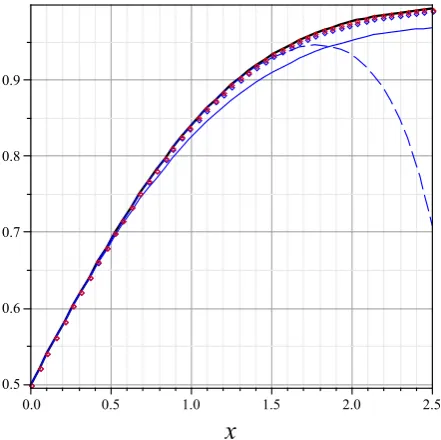
Figure 1: Comparison of the approximate solutions, given by (14) (blue dashed line), (23) (blue solid line), (24) (blue line of points) and (25) (red line), with the exact numerical solution to Eq. (4) (black line).
wherej ≥1. The exact solutions for the set of equations (11) with initial conditions (12) can be readily found as
Φ0(x) = 1 2+
x
√
2π,
Φ1(x) = − 1
√
2π x3 2·3,
Φ2(x) = 1
√
2π x5
2! 4·5 (13)
Φ3(x) = − 1
√
2π x7 3! 8·7...
Substituting all solutions (13) into equation (9), we obtain
Φ(x) =1 2 +
1
√
2π
x− x
3
2·3+
x5 2! 4·5−
x7 3! 8·7 +...
(14) The convergence of this solution is rather obvious, because formula (14) could be obtained merely from the decomposition
e−t
2
2 = 1−t
2
2 +
t4 4·2!−
t6 8·3!+...
in equation (4). Thus, such a simple homotopy yielded a rather expected result just coinciding with the approximation obtained by decomposition of the exponent into a Taylor se-ries. Acceptable accuracy of such an approximation can be achieved only by keeping a sufficiently large number of terms in this decomposition that is not always convenient. Obviously, we must somehow improve the homotopy in order to obtain a more accurate approximation for CDF.
x
0 0.5 1.0 1.5 2.0 2.5
[image:3.595.56.277.89.309.2]K0.0003 K0.0002 K0.0001 0
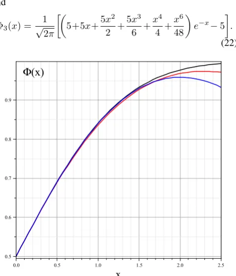
Figure 2: The absolute errors of the approximate solution given by equation (25), compared to the exact numerical solution to equation (4).
2.2
The case of improved homotopy
In this case, we build the homotopy according to the general procedure of the method, namely
Φ00(x) + Φ0(x) +p(x−1) Φ0(x) = 0, (15) wherep ∈ [0,1]. Then, substituting (8) into equation (15) and equating coefficients of like powers ofp, we obtain the following set of the linear differential equations:
p0 : Φ000+ Φ00= 0, (16)
p1 : Φ001+ Φ01+ (x−1) Φ00= 0, (17)
. . . .
pn : Φ00n+ Φ0n+ (x−1) Φ0n−1= 0, (18)
. . . .
Obviously, all successive approximations can be obtained rather easily. Solving equation (16) with the initial conditions (12), one can get
Φ0(x) = 1 2 +
1
√
2π 1−e
−x
. (19)
Substituting this function into equation (17), and taking into account (12), we obtain after integration that
Φ1(x) =
x2
2√2πe
−x. (20)
Then we can solve equation (18) forn = 2andn = 3 with initial conditions (12). The result is as follows
Φ2(x) = 1
√
2π−
1
2√2π
2 + 2x+x2+x 4
4
and
Φ3(x) = 1
√
2π
5+5x+5x 2
2 + 5x3
6 +
x4 4 +
x6 48
e−x−5
.
(22)
x
0.0 0.5 1.0 1.5 2.0 2.5
0.5 0.6 0.7 0.8 0.9
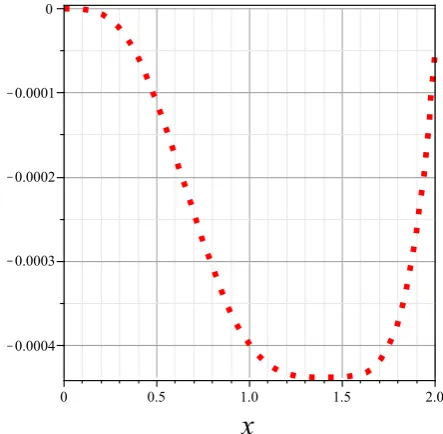
[image:4.595.51.290.92.372.2]F(x)
Figure 3: Comparison of the approximate solutions given by formula (32) forλ= 0.5(in blue) andλ= 1/√2(in red) with the exact numerical solution to Eq. (4) (in black).
According to equation (9) and the accuracy achieved in the caseΦ(x)≈Φ0(x) + Φ1(x), we obtain the following
approx-imate solution
Φ(x)≈ 1
2+ 1
√
2π
1−
1−x
2
2
e−x
, (23) by summing (19) and (20). Taking into account equations (19)-(21), we can obtain the next approximationΦ(x) ≈Φ0(x) + Φ1(x) + Φ2(x)as follows
Φ(x)≈ 1
2+ 1
√
2π
2−
2 +x+x 4
8
e−x
. (24) In the framework of the present study, we constrain our-selves to the next approximation, namely,Φ(x) ≈ Φ0(x) + Φ1(x) + Φ2(x) + Φ3(x). Due to equations (22) and (24), this
approximation is as follows
Φ(x)≈ 1
2 − 1
√
2π
3−
3 + 4x+5x 2
2 +
+5x 3
6 +
x4
8 +
x6
48
e−x
. (25) In order to demonstrate the accuracy of the method applied, the graphs of the approximate solutionsΦ(x)according (16) for different values ofλand the numerical solution to equation (4) via the Maple package are given in Fig. 1. The absolute error of the approximate solution (25), compared to the exact numerical solution to equation (4), is plotted in Fig. 2, and demonstrates a rather high level of accuracy for this approximation.
2.3
A one-parameter tuning of improved
homo-topy
In this case, we are going to introduce a real tuning parameter
λinto the homotopy (15) considered in the previous section, for example, as follows
Φ00(x) +λΦ0(x) +p(x−λ) Φ0(x) = 0. (26)
x
0.0 0.2 0.4 0.6 0.8 1.0 1.2 1.4 1.6 1.8 K0.009
[image:4.595.316.542.166.411.2]K0.008 K0.007 K0.006 K0.005 K0.004 K0.003 K0.002 K0.001 0.000
Figure 4: The absolute errors of the approximate solutions, given by equation (33) (in blue) and equation (34) (in red), compared to the exact numerical solution to equation (4).
As a result, the system of equations (16)-(18) transforms into the following set of linear equations
p0 : Φ000+λΦ00= 0, (27)
p1 : Φ001+λΦ10 + (x−λ) Φ00= 0, (28)
. . . .
pn : Φ00n+λΦ0n+ (x−λ) Φ0n−1= 0, (29)
. . . .
Solving equation (27) with the same initial conditions (12), we obtain
Φ0(x, λ) = 1 2+
1
λ√2π 1−e
−λx
. (30) Using this function in equation (28), and again taking into account (12), we can obtain that
Φ1(x, λ) = 1
λ√2π
λ2−1
λ2 1−(1 +λx)e −λx
+x 2
2 e −λx
.
(31) Taking into account equations (30) and (31), we can obtain the simplest one-step approximate solutionΦ(x, λ)≈Φ0(x, λ) + Φ1(x, λ)as follows
Φ(x, λ)≈1
2 + 1
λ√2π
2λ2−1
λ2 +
+
x2 2 −
λ2−1
λ x−
2λ2−1
λ2
e−λx
A single parameter that can be adjusted in (32) (for exam-ple, by using the NonlinearFit command from Maple Release 15) in order to obtain a good approximation isλ. As a con-sequence, this adjustment allows us to ignore a large number of successive terms in a good approximation. The graphs of the approximate solutions forΦ(x)given by equation (32) for
λ= 0.5andλ= 1/√2compared to the numerical solution to equation (4) are plotted in Fig.3.
x
0.0 0.5 1.0 1.5 2.0 2.5
0.5 0.6 0.7 0.8 0.9
[image:5.595.55.279.195.415.2]F(x)
Figure 5: Comparison of the approximate solutions given by equations (34) (red solid line) and (35) (red line of points) with the exact numerical solution to Eq. (4) (black line).
We present expression (32) in these two cases as the illustra-tive examples, when the formulae take the most simple form. Indeed, from (32) we have
Φ(x) =1 2 +
1
√
2π
"
x2+ 3x+ 4
e− x
2 −4
#
, (33)
whenλ= 0.5, and
Φ(x) =1 2 +
1 2√π
x2+√2xe
−√x
2, (34)
whenλ= 1/√2. The absolute errors of these approximations compared to the numerical solution of equation (4) are plotted in Fig. 4.
It should be noted that approximation (32), and, conse-quently, particular formulas (33) and (34), were obtained in a single iteration. It is clear that subsequent iterations will sig-nificantly improve the accuracy of the approximation, while at the same time complicating the expression for CDF. In view of the complexity of the general expression for the second itera-tion, we give here the following approximation for the case of theλ= 1/√2, which demonstrates the best result with relative simplicity of the expression in the above result. One can easily solve the linear equation (29) forn = 2 taking into account
Φ1(x,1/
√
2)forλ= 1/√2from (31), and then obtain the ap-proximate solutionΦ(x)≈Φ0(x) + Φ1(x) + Φ2(x)according
to (34) as follows
Φ(x) =1 2+
1
√
π
"
7− 7+3√2x+5 4x
2+
√
2 4 x
3+x4 8
!
e− x
√ 2
#
.
(35) The graphs of the approximate solutions forΦ(x)represented by equations (34) and (35) compared to the numerical solution to equation (4) are plotted in Fig. 5. The absolute error of the
x
0 0.5 1.0 1.5 2.0
K0.0004 K0.0003 K0.0002 K0.0001 0
Figure 6: The absolute error of approximate solution, given by equation (35), compared to the exact numerical solution to equation (4).
best approximation (35) compared to the numerical solution of equation (4) is plotted in Fig. 6. It can be seen from this figure that formula (35) provides a rather accurate result along with relative simplicity of its expression.
3
Conclusions
In this paper, we presented some approximate analytic solu-tions for the cumulative normal distribution obtained by using HPM. Formulae (25) and (35) provide the best approximations with low order relative errors. For example, one of the best approximation given by formula (35) for0 < x < 2 has an absolute error of less then4.5×10−4. Our approximations to
[image:5.595.316.538.230.447.2]REFERENCES
[1] N. Johnson, S. Kotz, and N. Balakrishnan, Continuous Univari-ate Distributions, Vol. 1,John Wiley&Sons, New York, 1994.
[2] M. Edous, O. Eidous. A Simple Approximation for Normal Distribution Function,Mathematics and Statistics, 6(4): 47-49, 2018.
[3] O. M. Eidous, and S. A. Al-Salman. One-Term Approximation for Normal Distribution Function,Mathematics and Statistics, 4(1): 15-18, 2016.
[4] H. Vazquez-Leal, R. Castaneda-Sheissa, et al. High Accurate Simple Approximation of Normal Distribution Integral, Mathe-matical Problems in Engineering, Vol. 2012, Article ID 124029, 2012. doi:10.1155/2012/124029.
[5] K. M. Aludaat, and M. T. Alodat. A Note on Approximating the normal distribution function,Applied Mathematical science, 2(9): 425-429, 2008.
[6] B. J. Bailey. Alternatives to hasting’s approximation to the in-verse of the normal cumulative distribution function,Applied statistics, 30(3): 275-276, 1981.
[7] G. Polya. Remarks on computing the probability integral in one and two dimensions, Proceeding of the first Berkeley sympo-sium on mathematicalstatistics and probability, 63-78, 1945.
[8] S. R. Bowling, M. T. Khasawneh, S. Kaewkuekool, and B. R. Cho. A Logistic approximation to the cumulative normal
dis-tribution,Journal of Industrial Engineering and Management, 2(1): 114-127, 2009.
[9] J. T. Lin. A simple Logistic approximation to the normal tail probability and its inverse, Applied Statistics, 39: 255-257, 1990.
[10] R. Yerukala, and N.K. Boiroju. Approximations to Standard Normal Distribution Function,International Journal of Scien-tific&Engineering Research, 6(4): 515-518, 2015.
[11] V. K. Shchigolev. Calculating Luminosity Distance versus Red-shift in FLRW Cosmology via Homotopy Perturbation Method,
Gravitation and Cosmology, 23(2): 142?48, 2017.
[12] J.-H. He. Homotopy perturbation technique, Comput. Meth. Appl. Mech. Eng., Vol. 178, 257?62, 1999.
[13] J.-H. He. A coupling method of homotopy technique and per-turbation technique for nonlinear problems, Int. J. Nonlinear Mech., 35(1): 37?3, 2000.
[14] J.-H. He. Homotopy perturbation method: a new nonlinear ana-lytical technique,Appl. Math. Comput., 135: 73?9, 2003.