Soil Temperature Manipulation to Study Global Warming
Effects in Arable Land: Performance of Buried
Heating-cable Method
Raveendra H. Patil
1,*, Mette Laegdsmand
2, Jørgen E. Olesen
3, John R. Porter
41University of Florida, Gainesville, Florida, 32611-0570, USA 2Unisense FertiliTech A/S, Tueager 1, DK-8200, Aarhus N, Denmark 3Department of Agroecology, Aarhus University, 8830 Tjele, Denmark
4University of Copenhagen, DK-2630 Taastrup, Denmark *Corresponding Author: [email protected]
Copyright © 2013 Horizon Research Publishing All rights reserved.
Abstract
Buried heating-cable method for manipulating soil temperature was designed and tested its performance in large concrete lysimeters grown with the wheat crop in Denmark. Soil temperature in heated plots was elevated by 5 oC compared with that in control by burying heating-cable at 0.1 m depth in a plough layer. Temperature sensors were placed at 0.05, 0.1 and 0.25 m depths in soil, and 0.1 m above the soil surface in all plots, which were connected to an automated data logger. Soil-warming setup was able to maintain a mean seasonal temperature difference of 5.0 ± 0.005 oC between heated and control plots at 0.1 m depth while the mean seasonal rise in soil temperature in the top 0.25 m depth (plough layer) was 3 oC. Soil temperature incontrol plots froze (≤ 0 oC) for 15 and 13 days respectively at 0.05 and 0.1 m depths while it did not in heated plots during the coldest period (Nov-Apr). This study clearly showed the efficacy of buried heating-cable technique in simulating soil temperature, and thus offers a simple, effective and alternative technique to study soil biogeochemical processes under warmer climates. This technique, however, decouples below-ground soil responses from that of above-ground vegetation response as this method heats only the soil. Therefore, using infrared heaters seems to represent natural climate warming (both air and soil) much more closely and may be used for future climate manipulation field studies.
Keywords
Climate Change, Climate Manipulation, Soil Warming, Heating Cables, Soil Temperature, Agro-Ecosystems1. Introduction
Between 1850 and 2000, the global mean air temperatures have risen by 0.74oC and are projected to increase further by 0.3oC to 6.4oC by the end of 21st century, subject to regional
variations, (IPCC 2007). In northern latitudes rise in temperatures are expected to be on the high end of these projections, particularly during winter (Folland et al., 2001). Northern Europe, for instance, has already witnessed a warming of around 0.7−1.0oC between 1970 and 2000 (Walther et al., 2002), which suggests that with business as usual temperatures might rise beyond 6oC by the end of 21st century. In Denmark, for the period 2000-2010 itself compared with 1960-1990, average winter and summer temperatures have respectively risen by 1.5oC and 1.1oC (Kristensen et al., 2011), a trend showing relatively more warming during winter than in summer.
only reduce N losses to the environment, but also help fix more CO2 by the crop and compensate for CO2 emissions from enhanced soil respiration and help mitigate global warming (McGuire et al., 1992; Melillo et al., 2002).
Therefore, a number of soil temperature manipulation studies have been carried out in the last two decades on either perennial forest tree species or grasslands from mid to high latitudes. These studies have shown increased rate of litter decomposition (van Cleve et al., 1990), CO2 fluxes (Peterjohn et al., 1994), nitrification (Verburg et al., 1999), and N mineralization and its availability (van Cleve et al., 1990, Bonan and van Cleve, 1992, Jonasson et al., 1999, Rustad et al., 1996, Verburg et al., 1999, Melillo et al., 2002) in response to increase in soil temperature. Similarly, increased concentrations of NO3-N in the soil solution resulting in increased N leaching (Lukewille and Wright, 1997) and N2O emissions (Sitaula and Bakken, 1993) to soil warming have also been recorded. Rise in soil temperature affects physical properties vis-à-vis ion adsorption and soil moisture (Peterjohn et al., 1993 and 1994; Hantschel et al., 1995, Pajari, 1995, Rustad and Fernandez, 1998) as well as microbial activities controlling soil respiration and N mineralization.
Soil temperature influences phenology. In wheat for instance, temperature near the apical meristem directly affects the rate of leaf appearance until the end of stem elongation (Jamieson et al., 1995). This is because during the early developmental period of wheat, both the seedling apex
and the zone of leaf extension are located either below or near the soil surface (Hay, 1978, Kemp, 1980). Positive responses on plant growth and biomass production, and nutrient absorption in response to elevated soil temperature have also been documented (e.g. Stone et al., 1999, Awal and Ikeda 2003, Frantz et al., 2004, Kanso, 2010).
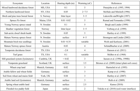
Table 1 lists soil temperature manipulation studies carried out using only heating-cables, which clearly shows that a large number of studies have been carried out on perennial ecosystems (forests and grasslands) compared with arable land. Furthermore, the range of increase in soil temperature
[image:2.595.63.547.435.748.2](2.0−7.5 oC), the depth at which heating-cables were placed (surface to 2 m deep) varied between these studies. If the objectives were to look at soil biogeochemical processes (e.g., soil respiration, soil N cycling) in arable soils and increase the soil temperature using heating-cables, we argue here that it would be more appropriate to bury the heating-cables in plough layer, which is biologically the most active zone (e.g., biogeochemical processes and root density as well as their activities). Moreover, placing heating-cables on the surface has shown difficulties in controlling the temperature at a targeted level (e.g. Kanso, 2010). Therefore, we made a soil temperature manipulation study employing a buried heating-cable method to test its performance and this methodology paper describes the design, layout and performance of ‘buried heating-cable method’, and discusses limitations in comparison to other alternative methods.
Table 1. Brief summary of soil temperature manipulation studies carried out using only heating-cables Ecosystem Location Heating depth (m) Warming (oC) References Mixed hardwood deciduous forest MS, USA 0.1 5 Peterjohn et al. (1993, 1994)
Northern hardwood forest NY, USA 0.05 2−7.5 McHale and Mitchell (1996) Birch and pine trees boreal forest S. Norway litter layer 3−5 Lukewille andWright (1997)
Spruce Fir forest Maine, USA 0.01−0.02 5 Rustad and Fernandez (1998)
Young Norway spruce stand N. Sweden 0.1 5 Bergh and Linder (1999)
Heather vegetation forest Norway litter layer 3−5 Verburg et al. (1999) Sub-arctic dwarf shrub heath N. Sweden 0.05 5 Hartley et al. (1999) Mature Norway spruce forest N. Sweden surface 4−5 Stromgren and Linder (2002) Mountain birch tree seedlings N. Sweden 0.01−0.35 variable Weih and Karlsson, (2001) Mature Norway spruce forest Austria 0.03 4 Schindlbacher et al. (2009)
Temperate deciduous forest TN, USA ~2.0 4 Hanson et al. (2011)
Turf grass TX, USA 0.1 variable McBee et al. (1968)
Hill grassland system (lysimeters) Cumbria, UK < 0.02 3 Ineson et al. (1998a, 1998b) Temperate grassland Scotland, UK surface 3.5 Briones et al. (2009) (intact plant-soil cores)
Wheat crop land Munich, Germany 0.02 3 Hantschel et al. (1995)
Arable fallow and wheat fields Germany surface 3 Kamp et al. (1998)
Soil from wheat and maize field York, UK 0.04 3 Hartley et al. (2007) Arable land soil (lysimeters) Munich, Germany surface 3 Reth et al. (2009)
Spring wheat arable land Germany surface 2.5 Kanso (2010)
2. Material and Methods
2.1. Study Site and Experimental Facility
This study was made at Aarhus University, Foulum, Denmark (56º29´N, 9º34´E). We used 32 concrete lysimeters each of 1 m2 in surface area (1m in length × 1m in width) and 1.5 m deep. These 32 lysimeters were built >20 years ago in four rows with each row having eight lysimeters (8 × 4) next to each other, and filled with loamy sand soil (TypicHapludult; FAO classification) in the top 1.4 m depth while the bottom 0.1 m was filled with gravel for free drainage. Since construction these lysimeters have been used for experimentation on a regular basis, which has enabled the soil to settle down firmly closely representing the soil from surrounding fields.The top surface of these lysimeters is at level with the surrounding arable land. The inner side of each concrete lysimeter was coated with a layer of epoxy which prevented percolation of water across lysimeter walls from all the four sides. More details on the soil properties and climatic conditions of the site are provided in Patil et al. (2010aand 2010b).
2.2. Soil-Warming Setup and Control Unit
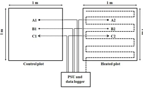
[image:3.595.315.548.74.218.2]Of the total 32 lysimeters (referred to as plots in the text), 16 randomly selected ones (4 from each row) were installed with insulated heating-cables representing heated plots, while the remaining 16 acted as unheated (control) plots. During tillage (ploughing up to 0.2 m depth), the soil from the top 0.1 m depth of 16 heated plots was taken out and kept in separate plastic trays. A single cord of 7.35 m long heating-cable was moulded into eight rows at 0.125 m spacing and placed at 0.1 m depth (Figure 1). The insulated heating-cables were made of ‘Teflon-Copper-Teflon’ wire with an outer diameter of 0.005 m. Each of these 16 heating-cables was separately connected to a power supply unit (Figure 2). In order to achieve similar physical disturbance in all the plots, the soil from remaining 16 control plots was also removed and returned, but no heating-cable was placed. All 32 plots were left unused for a week to allow the soil from the top 0.1 m depth to settle down before winter wheat seeds were sown at a row spacing of 0.125 m on October 10, 2008.
Figure 1. Layout of heating-cable in heated plots at 0.1 m depth.
Figure 2. Bird’s eye view of soil-heating setup installed in heated and control plots at the study site. A1, B1 and C1 are the temperature sensors in control plot respectively placed at 0.05, 0.1 and 0.25 m depths, A2, B2 and C2 are the temperature sensors in heated plot respectively placed at 0.05, 0.1 and 0.25 m depths, and all were connected to data-logger through sensor cables, which in turn were connected to an automated power supply unit (PSU). Heating-cable was buried below the crop row at 0.1m depth only in heated plots as shown in Figure 1 and connected to PSUs.
Heating of soil in all the 16 heated plots was started on October 23, 2008, 13 days after sowing, and soil temperature in all the heated plots at 0.1 m depth was maintained at 5 oC above the temperature in control plots at the same depth all through the study period (until August 15, 2009).The heating system was controlled and monitored by an automated power supply unit and a data logger board that was connected to all the plots (32 in total) via temperature sensors (Campbell Scientific Inc., Germany). The data logger was separately fed with soil temperature at 0.1 m depth from each of 16 heated plots, which was compared with soil temperature at 0.1 m depth from their respective 16 referenced control plots. Each heated plot was paired with an unheated reference plot (at 0.1 m depth) from the same replication (row). If the difference in mean temperature at 0.1 m depth between heated plot and its reference control plot was <5 oC the automated data logger turned on the power supply to warm the heated plot until the temperature difference reached 5 oC; conversely, if the difference in temperature between heated
and its referenced control plot was ≥5 oC the automated data logger immediately turned off the power supply to that particular heated plot. This was achieved through temperature sensors installed in all the heated and control plots at 0.1 m depth (Figure 2).
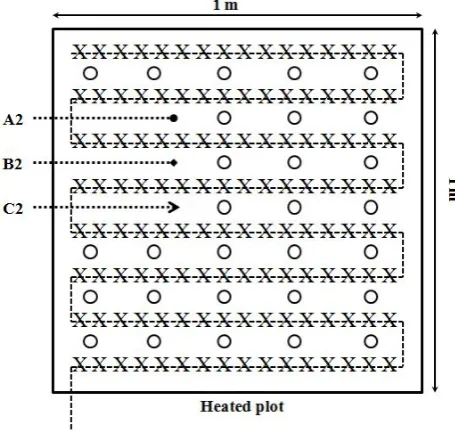
In addition to placing temperature sensors at 0.1 m depth in all the 32 plots, we installed temperature sensors at 0.05 m and 0.25 m depth, as well in two control and two heated plots, which enabled us to record soil temperature at different depths in the plough layer (0.05, 0.1 and 0.25 m; Figure 2) all through the study period. The sensors (0.1 m long metal cylinders) were placed horizontally between heating-cable rows, which ran exactly below the crop rows as shown in Figure 3. Temperature sensors were also placed above the soil in four heated and four control plots to record air temperature at 0.10 m above the soil surface. This was done by placing the 0.1 m long sensor part vertically above the
[image:3.595.68.287.611.738.2]These sensors enabled us to record the difference in air temperature between heated and control plots. These vertically placed sensors were covered with a shield with natural ventilation to protect from effects of radiation and rain. The entire temperature sensor cables (48 in total) coming from 32 plots were connected to the data logger as shown in Figure 2. An automated and remotely controlled power supply unit with the data logger enabled to monitor temperature continuously at 15s interval, which, in turn, helped the unit to maintain a constant temperature difference of 5 oCbetween heated and control plots. The data on soil temperature from each of the sensors were stored automatically every 15 min and averaged for each day, hence only the daily mean values were used for interpretation of results.
Figure 3. Bird’s eye view of heated plot showing layout of heating-cable (dotted line) exactly below the crop rows (X). The figure also shows the points of soil measurement (O) collected from top 0.3 m depth at monthly interval during the study period. Soil samples were not collected from near and around the temperature sensors (A2, B2 and C2). Control plots looked the same but without heating-cable.
Temperature at the soil-air interface (on the soil surface) was also measured manually on March 26, 28, 30 and April 2,
2009 between 11 AM and 2 PM (local time) to record the difference in temperature between heated and control plots at the surface, and as well as between the soil surface and at 0.10 m above the surface. This was done by measuring the temperature from between the crop rows, and from randomly selected two heated and two control plots. The mean values (with n = 42 points of measurement per plot × 2 plots) are presented here. As the heating-cable ran directly below the crop rows (Figure 3), it was important also to manage a uniform heating across the plot and between the rows in each heated plot. Therefore, spatial distribution of temperature within the heated plot at 0.1 m depth was also measured manually from two randomly selected heated plots on February 4 and March 4 between 11 AM and 2 PM (local time). This was done by measuring the temperature at 0.1 m × 0.1 m grids across the plot with a total of 81 measurement points per plot, and the mean values for each grid point from both the plots are referred to in the discussion. During this study, in addition to soil temperature treatment, the lysimeters were also subject to another treatment factor; that of changes in precipitation patterns (both amount and number of events) , and we studied the resulting responses of the wheat crop and soil N availability/flows (Patil et al., 2010a and 2010b).
3. Results and Discussion
The heating-cable placed in each heated plot occupied 0.04% of the total physical space per plot at 0.1 m depth. Effects of this physical occupation of space by the heating-cable or any alteration (disturbance) caused to the soil environment or soil processes by placing heating-cables were not studied as it has been shown to be non-significant in many studies in the past (e.g. Rustad and Fernandez, 1998; McHale et al., 1998; Hartley et al., 1999; Schindlbacher et al. 2009). The soil-warming setup was operational all through the study period (October 23, 2008 until August 15, 2009) without any failures or interruptions, including the freezing and thawing cycles during winter and early spring.
[image:4.595.125.487.588.726.2]3.1. Soil Temperature in the Plough Layer
The soil-warming setup used in this study maintained a mean seasonal temperature difference of 5.0 ±0.005 oC (n= 277 days) between heated and control plots at 0.1 m depth (Figure 4). However, the soil temperature at 0.05 m and 0.25 m depths responded differently to the heating at 0.1 m depth. The soil temperature at 0.05 m depth, in particular, also showed much larger daily temperature fluctuations as it was exposed to variations caused by direct solar radiation and air temperature, whereas soil temperature at deeper layers (0.25 m depth) was relatively more stable. For instance, the rapid
increase in air temperature during summer (e.g. July−August)
caused the soil temperature in heated plots at 0.05 m depth to rise beyond 5 oC difference, as this layer experienced heating from both the above- (air temperature) and below-ground (soil temperature). For the whole study period, on average, a 4.04 ± 0.037 oC(n= 277 days) increase at 0.05 m depth and a 2.74 ± 0.01 oC (n= 277 days) increase at 0.25 m were achieved when the soil temperature at 0.1 m depth was increased by 5 oC (Table 2). Overall, the mean seasonal rise in temperature in the plough layer (top 0.25 m) was 3.93 ± 0.02 oC with 0.11 oC lower during winter (3.82 oC; Oct. 23 to Mar. 31) and 0.13oC higher during summer (4.06 oC; Apr. 1 to Aug. 15). This shows that the soil-warming setup used in this study affected the entire plough layer vis-à-vis conductive heat with an average increase close to 4 oC. The small variation in temperature over time also prove (i) the applicability of insulated heating-cable equipment for elevating soil temperature, and (ii) placing the heating-cable within plough layer and not on or just below the surface, enables high degree of control on soil temperature. While none of the methods employed in the past proved to be perfect (Shaver et al. 2000), the methodology chosen should be simple in design and cost effective to be easily replicable, inexpensive, reliable and durable even under harsh climatic conditions with minimal artefact effects (Marion et al.,
1997).
3.2. Effect of Soil-Warming on Air Temperature
Soil-warming increased the mean seasonal air temperature of heated plots (measured at 0.10 m above the soil surface) marginally by 0.2 oCcompared with that of control plots (Table 2). The minimum and maximum difference in mean temperature between heated and control was respectively 0.02 oC(March) and 0.43oC (July). However, temperature measured at the soil-air interface showed much larger difference between heated and control plots with the former plots recording, on average, 2 oC warmer than latter plots (Figure 5), but this difference dropped to <0.1 oC when
measured at 0.05−0.15 m above the surface. This was due to
[image:5.595.320.550.317.456.2]latent heat transfer through increased crop evapotranspiration (data not shown here) and might also likely be due to decimation of sensible heat mediated through wind and turbulence above the soil surface.
Figure 5. Temperature (oC) at soil-air interface for heated and control plots measured on four dates and the overall mean. Vertical error bars indicate ±1 standard error with n = 32 (2 observations per row × 8 rows per plot × 2 plots).
Table 2. Monthly mean temperatures (oC) at 0.1 m above soil surface, and at 0.05 m, 0.1 m and 0.25 m below soil surface in heated and control plots 0.1 m above
soil surface 0.05 m below soil surface 0.1 m below soil surface 0.25 m below soil surface
Month Control Heated Control Heated Control Heated Control Heated
Oct 6.7 7.2 7.2 11.0 7.6 12.5 9.3 12.2
Nov 4.9 5.0 4.7 8.5 5.1 10.2 7.2 9.9
Dec 2.1 2.2 2.7 6.5 3.0 8.0 5.0 7.7
Jan 1.0 1.0 1.2 4.9 1.3 6.3 3.1 5.8
Feb 1.1 1.2 1.2 4.9 1.0 6.0 2.6 5.3
Mar 4.1 4.1 4.4 8.2 4.3 9.3 5.7 8.4
Apr 10.1 10.4 10.9 14.6 10.3 15.3 11.2 13.8
May 12.6 12.8 12.8 16.8 12.3 17.3 13.6 16.3
Jun 15.5 15.7 15.4 20.1 15.3 20.3 16.1 18.9
Jul 18.5 18.9 19.0 23.9 18.8 23.7 19.7 22.7
Aug 18.1 18.2 19.9 25.2 19.5 24.6 20.5 23.4
[image:5.595.71.543.539.754.2]3.3. Spatial Distribution of Soil Temperature
[image:6.595.318.545.135.248.2]The spatial distribution of temperature at 0.1 m depth in heated plots was measured on February 4 and March 4, 2009. On February 4 the mean temperature at 0.1 m depth was 3.6 oC (± 0.007; n=81) with the minimum and maximum values respectively ranging between 3.4 oC and 3.8 oC. Similarly, on March 4 the mean temperature at 0.1 m depth was 10.5 oC (± 0.011; n=81) with the minimum and maximum values respectively ranging between 10.3 oC and 10.7 oC. The difference in minimum and maximum values recorded during these two measurements was <0.5 oC. This small observed variation in soil temperature may in part have been caused by variation in soil moisture across plot. Overall, we could achieve uniform heating across the plot at 0.1 m depth. However, the temperature on and along the heating-cable might have been on higher side than the one sensed by the temperature sensors placed between the heating-cable rows (or crop rows). We, however, did not measure the former one (on/near the buried heating-cable) to avoid physical damage to the heating-cable.
Figure 6. Daily mean soil temperature (oC) at 0.05m depth in heated and control plots (n=8) during the heating period
3.4. Effect on Soil Freezing and Thawing
The soil in heated plots did not freeze (≤0 oC), while the soil temperature in control plots at 0.05 m and 0.1 m reached
≤0 oCon several occasions and each time for several days (Figure 6 and 7). In control plots the number of days with ≤ 0
oC daily mean temperature were respectively 15 and 13 at 0.05 m and 0.1 m depth, which meant soil-warming kept the soil unfrozen and wet in heated plots all through the winter period. These freezing events (≤ 0 oC) occurred between November 23 and February 16 at 0.05 m depth, and between January 5 and February 20 at 0.1 m depth. At 0.25 m depth, however, no freezing events were recorded even in control plots. Kamp et al. (1998) also recorded significant reduction in number of frost days (top 0.5 m depth) in heated plots (+3 oC in the top 0.1 m soil) compared with the one in control plots on both fallow and wheat fields. Complete or partial reduction in frost days during winter/spring under warmer climates in northern temperate regions may enhance decomposition of SOM and N cycling, and potentially increase the mineral N flows through leaching or as N2O emissions, if not taken up by above-ground vegetation (Patil
[image:6.595.62.293.337.455.2]et al., 2010a and 2010b). Therefore, in depth studies for assessing the impacts of complete or partial reduction in frost days on decomposition of SOM, soil N mineralization and crop response from temperate arable crops are required.
Figure 7. Daily mean temperature (oC) at 0.1 m depth in heated and control plots (n=8) during the heating period
3.5. Limitations of Soil-Warming Studies
Different techniques or methods have been used in the past, including the one described in this paper (buried heating-cable method) and listed in Table 1, for manipulating soil temperature. While the objective of these methods was to simulate projected future climate with minimum effects on other climatic factors (e.g., rainfall, solar radiation, shade, wind, humidity), many of these methods have failed to do so. For instance, heating of soil columns with hot fluid supply (Ineson and Benham, 1991) fail to maintain constant temperature difference in larger plots and over longer period of time. Similarly, warming with infrared reflectors or heaters above crop canopy heats crop canopy, but fails to raise soil temperature at lower depths, especially under extreme cold climates of northern latitudes and thickly covered vegetation (Harte et al., 1996; Aronson and McNulty, 2009; Hanson et al., 2011). Soil-warming using greenhouses and open top chambers, on the other hand, alter micro-climate (e.g. wind speed, radiation and humidity) affecting physiological processes of plants under study. Similarly, using covers and roofs manipulate (reduce) incoming solar radiation (Chapin and Shaver, 1985; Beier et al., 2004).
ambient (current) temperatures (Hantschel et al., 1995), except during early vegetative period. This directly affects root activities (e.g. Kandeler et al., 1998; Briones et al., 2009), and the rate of SOM decomposition and mineralization processes (van Cleve et al., 1990; Peterjohn et al., 1993), but might show little or no effect on above-ground vegetation. Therefore, buried heating-cable method fits well if study was undertaken to investigate the response of only soil vis-à-vis soil nutrient cycling, nutrient flows and soil-inhabiting organisms to elevated soil temperature.
4. Perspective
It is important to continue perform climate manipulative experiments to better understand direct and indirect impacts of warmer climate on different ecosystems, which would intern help further improve both climate and crop models. However, different methods employed to elevate temperature under field conditions do have artifact effects (Aronson and McCulty, 2009) and tend to be logistically expensive to maintain depending on the climate and ecosystem chosen to study. Therefore, the challenge is to design a cost and energy efficient method which achieves rise in both air and soil temperature like a normal incoming solar radiation with minimal artifact effects. In this context, using infrared heaters seems to represent climate warming more like a normal solar radiation (Wan et al., 2002; Aronson and McCulty, 2009; Kimball et al., 2008 and 2012). Infrared heaters hung in hexagonal or octagonal way above crop canopy on experimental plots enable uniform transfer of thermal radiation, and warms both crop and soil closely representing warming caused by normal solar radiation (Kimball, 2008; Luo et al, 2010; Wall et al, 2011) which is critical to study climate warming under field conditions. This is achieved by enhancing downward infrared radiation which elevates air temperature (sensible heat), increase evapotranspiration (latent heat) and warm soil (conductive heat) (Harte and Shaw, 1995; Shaver et al., 2000). Infrared heaters also seem to be more efficient, reliable and enable uniform heating of experimental plots with least shading effect (Kimball et al., 2012). However, the only concern about use of infrared heaters hung above crop canopy is lack of soil warming under thickly or fully covered vegetation. This, however, could be overcome by combining infrared canopy heating with buried-cable soil heating.
REFERENCES
[1] Aerts, A., Cornelissen, J.H.C., Dorrepaal, E., 2006. Plant performance in a warmer world: general responses of plants from cold, northern biomes and the importance of winter and spring events. Plant Ecol. 182(1), 65–77.
[2] Aronson, E.L., McNulty, S.G., 2009. Appropriate experimental ecosystem warming methods by ecosystem.
Agr.Forest Meteorol. 149, 1791–1799.
[3] Awal, M.A., Ikeda T. (2003): Controlling canopy formation, flowering, and yield in field-grown stands of peanut (Arachishypogaea L.) with ambient and regulated soil temperature. Field Crops Res. 81(2-3), 121–132
[4] Beier, C., Emmett, B., Gundersen, P., Tietema, A., Penuelas, J., Estiarte, M., Gordon, C., Gorissen, A., Llorens, L., Roda, F., Williams, D., 2004. Novel approaches to study climate change effects on terrestrial ecosystems in the field: Drought and passive nighttime warming. Ecosystems 7, 583−597. [5] Bergh, J., Linder, S., 1999. Effects of soil warming during
spring on photosynthetic recovery in boreal Norway spruce stands. Global Change Biol. 5, 245−253.
[6] Bonan, G.B., van Cleve K., 1992. Soil temperatures, nitrogen mineralization, and carbon source-sink relationships in boreal forests. Can. J. For. Res. 22, 629−639.
[7] Briones, M.J.I., Ostle, N.J., McNamara, N.P., Poskitt, J., 2009. Functional shifts of grassland soil communities in response to soil warming. Soil Biol. Biochem. 41(2), 315−322.
[8] Chapin, F.S., Shaver, G.R., 1985. Individualistic growth response of tundra plant species to environmental manipulations in the field. Ecology 66, 564–576.
[9] Ellert, B.H., Bettany, J.R., 1992. Temperature dependence of net nitrogen and sulfur mineralization. Soil Sci. Soc. Am. J. 56: 1133–1141.
[10] Fisk, M.A., Schmidt, S.K., 1996. Microbial response to nitrogen additions in alpine tundra soil. Soil Biol. Biochem. 28(6), 751–755.
[11] Folland, C.K, Karl, T.R., 2001. Observed Climate Variability and Change. In: Climate Change 2001: The Scientific Basis. Contributionof Working Group I to the Third Assessment Report of the Intergovernmental Panel on Climate Change Houghton JT, Ding Y, Griggs DJ, Noguer M, van der Linden PJ, Dai X, Maskell K, Johnson CA (eds). Cambridge University Press, pp. 99–181.
[12] Frantz, J.M., Cometti, N.N., Bugbee, B., 2004. Night temperature has a minimal effect on respiration and growth in rapidly growing plants. Annals Bot-London 94(1), 155–166. [13] Hanson, P.J., Childs, K.W., Wullschleger, S.D., Riggs, J.S.,
Thomas, W.K., Todd, D.E., Warren, J.M., 2011. A method for experimental heating of intact soil profiles for application to climate change experiments. Glob. Change Biol. 17(2), 1083–1096.
[14] Hantschel, R., Kamp T., Beese F., 1995.Increasing soil temperature to study global warming effects on the soil nitrogen cycle in agroecosystems. J. Biogeogr. 22(2-3), 375−380.
[15] Harte, J., Rawa, A., Price, V., 1996. Effects of manipulated soil microclimate on mesofaunal biomass and diversity. Soil Biol. Biochem. 28(3), 313–322.
[16] Harte, J., Shaw, R., 1995. Shifting dominance within a montane vegetation community, results of a climate-warming experiment. Science 267, 876−880.
[18] Hartley, A.E., Neill, C., Melillo, J.M., Crabtree, R., Bowles, F.P., 1999. Plant performance and soil nitrogen mineralization in response to simulated climate change in subarctic dwarf shrub heath. Oikos 86, 331–343.
[19] Hay, R.K.M., 1978. Seasonal changes in the position of the shoot apex of winter wheat and spring barley in relation to the soil surface. J. Agric. Sci. 91(1), 245–248.
[20] Hillier, S.H., Sutton, F., Grime, J.P., 1994.A new technique for experimental manipulation of temperature in plant communities. Funct. Ecol. 8(6), 755−762.
[21] Ineson, P., Benham, D.G., 1991. Field experimental study of the effects of global warming on C turnover in upland soils. Tiger project T91/I.2/5A T91/61. Institute of Terrestrial Ecology – Merlewood Research Station, Grange-over-Sands, UK
[22] Ineson, P., Benham, D.G., Poskitt, J., Harrison, A.F., Taylor, K., Woods, C., 1998. Effects of climate change on nitrogen dynamics in upland soils. 2. A soil warming study. Glob. Change Biol. 4(2), 153–162.
[23] IPCC., Intergovernmental Panel on Climate Change, 2007. Working Group I: the physical science basis. Summary for policymakers. In: Solomon, S., Qin, D., Manning, M., Chen, Z., Marquis, M., Averyt, K.B., Tignor, M., and Miller, H.L. (Eds), Climate change 2007, Cambridge University Press, Cambridge, UK.
[24] Jamieson, P.D., Brooking, I.R., Porter, J.R., Wilson, D.R., 1995. Prediction of leaf appearance in wheat: a question of temperature. Field Crops Res. 41(1), 35−44.
[25] Jeppesen, E., Kronvang, B., Olesen, J.E., Audet, J., Søndergaard, M., Hoffmann, C.C., Andersen, H.E., Lauridsen, T.L., Liboriussen, L., Larsen, S.E., Beklioglu, M., Meerhoff, M., Ozen, A., Ozkan, K., 2011. Climate change effects on nitrogen loading from catchment: implications for nitrogen retention, ecological state of lakes and adaptation. Hydrobiologia 663(1), 1–21.
[26] Jonasson, S., Michelsen, A., Schmidt, I.K., Nielsen, E.V., 1999. Responses in microbes and plants to changed temperature, nutrient and light regimes in the arctic. Ecology, 80(6), 1828–1843.
[27] Kamp, T., Steindl, H., Hantschel, R.E., Beese, F., Munch, J.-C., 1998. Nitrous oxide emissions from a fallow and wheat field as affected by increased soil temperatures. Biol. Fert. Soils, 27(3), 307–314.
[28] Kandeler, E., Tscherko, D., Bardgett, R.D., Hobbs, P.J., Lampichler, C., Jones, T.H., 1998. The response of soil microorganisms and roots toelevated CO2 and temperature in a terrestrial model ecosystem. Plant Soil 202(2), 251–262. [29] Kanso, F., 2010.Effect of root zone temperature and changes
in precipitation on yield components and yield formation in spring wheat (Triticum aestivum L. cv. Triso). M.Sc. Thesis submitted to the University of Hohenheim, Germany, p. 62. [30] Kemp, D.R., 1980. The location and size of the extension
zone of emerging wheat leaves. New Phytologist, 84(4), 729–737.
[31] Kimball, B.A., Conley, M.M., Lewin, K.F., 2012. Performance and energy costs associated with scaling infrared heater arrays for warming field plots from 1 to 100 m. Theoretical and Applied Climatology, 108(1-2), 247−265.
[32] Kimball, B.A., Conley, M.M., Wang, S., Lin, X., Luo, C., Morgan, J., Smith, D., 2008. Infrared heater arrays for warming ecosystem field plots. Glob. Change Biol. 14(2), 309−320.
[33] Kristensen, K., Schelde, K., Olesen J.E., 2011. Winter wheat yield response to climate variability in Denmark. J. Agric. Sci. 149(1), 33−47.
[34] Kudernatsch, T., Fischer, A., Bernhardt-Romermann, M., Abs, C., 2008. Short-term effects of temperature enhancement on growth and reproduction of alpine grassland species. Basic and Applied Ecology, 9(3), 263–274.
[35] Lukewille, A., Wright, R.F., 1997. Experimentally increased soil temperature causes release of nitrogen at a boreal forest catchment in southern Norway. Glob. Change Biol. 3(1), 13−21.
[36] Luo, C., Xu, G., Chao, Z., Wang, S., Lin, X., Hu, Y., Zhang, Z., Duan, J., Cang, X., Su, A., Li, Y., Zhao, X., Du, M., Tang, Y., Kimball, B., 2010. Effect of warming and grazing on litter mass tool and temperature sensitivity of litter and dung mass loss on the Tibetan plateau.Glob. Change Biol., 16(5), 1606−1617.
[37] Marion, G.M., Henry, G.H.R., Freckman, D.W., Johnstone, J., Jones, G., Jones, M.H., Levesque, E., Molau, U., Mølgaard, P., Parsons, A.N., Svoboda, J., Virginia, R.A., 1997. Open-top designs for manipulating field temperature in high-latitude ecosystems. Glob. Change Biol. 3 (Suppl. 1): 20–32.
[38] McBee, G.G., McCune, W.E., Beerwinkle, K.R., 1968. Effect of soil heating on winter growth and appearance of Bermudagrass and St. Augustinegrass. Agronomy Journal, 60(2), 228−232.
[39] McGuire, A.D., Melillo, J.M., Joyce, L.A., Kicklighter, D.W., Grace, A.L., Moore, B. III., Vorosmarty, C.J. 1992. Interactions between carbon and nitrogen dynamics in estimating net primary productivity for potential vegetation in North America. Global Biogeochem. Cycles 6(2), 101−134. [40] McHale, P.J., Mitchell, M.J., 1996. Disturbance effects on
soil solution chemistry due to heating cable installation. Biol. Fert. Soils 22(1–2), 40–44.
[41] McHale, P.J., Mitchell, M.J., Bowles, F.P., 1998. Soil warming in a northern hardwood forest: trace gas fluxes and leaf litter decomposition. Can. J. Forest Res. 28(9), 1365−1372.
[42] Melillo, J.M., Steudler, P.A., Aber, J.D., Newkirk, K., Lux, H., Bowles, F.P., Catricala, C., Magill, A., Ahrens, T., Morrisseau, S., 2002.Soil warming and carbon-cycle feedbacks to the climate system. Science 298(#5601), 2173–2176.
[43] Pajari, B., 1995. Soil respiration in a poor upland site of Scots pine stand subjected to elevated temperatures and atmospheric carbon concentration. Plant Soil 168− 169(1), 563−570.
[44] Patil, R.H., Laegdsmand, M., Olesen, J.E., Porter, J.R., 2010a. Growth and yield response of winter wheat to soil warming and rainfall patterns. J. Agr. Sci. 148(5), 553−566. [45] Patil, R.H., Laegdsmand, M., Olesen, J.E., Porter, J.R.,
139(1−2), 195−205.
[46] Peterjohn, W.T., Melillo, J.M., Steudler, P.A., Newkirk, K.M., Bowles, F.P., Aber, J.D., 1994. Responses of trace gas fluxes and N availability to experimentally elevated soil temperatures. Ecol. Appl. 4(3), 617–625.
[47] Peterjohn, W.T., Melillo, J.M., Bowles, F.P., Steudler, P.A., 1993. Soil warming and trace gas fluxes: experimental design and preliminary flux results. Oecologia 93(1), 18–24.
[48] Reth, S., Graf, W., Reichstein, M., Munch, J.C., 2009.Sustained stimulation of soil respiration after 10 years of experimental warming.Environmental Research Letters, 4(2/024005), pp 1−5.
[49] Rosenzweig, C., Parry, M.L., 1993. Potential impacts of climate change on world food supply: a summary of a recent international study. In: Kaiser HM, Drennen TE (eds) Agricultural dimensions of global climate change. St. Lucie Press, Delray Beach, pp 87–116.
[50] Rustad, L.E., Fernandez, I.J., Arnold, S., 1996. Experimental soil warming effects on C, N, and major element cycling in a low elevation spruce-fir forest soil. In: Hom J, Birdsey R, O’Brien K (eds) Proceedings – 1995 Meeting of the Northern Global Change Programm. Gen Tech Rep NE–214. USDA Forest Service, PA, pp 132–139.
[51] Rustad, L.E., Fernandez, I.J., 1998. Experimental soil warming effects on CO2 and CH4 flux from a low elevation spruce-fir forest soil in Maine, USA. Glob Change Biol., 4(6), 597–605.
[52] Rustad, L.E., Campbell, J.L., Marion, G.M., Norby, R.J., Mitchell, M.J., Hartley, A.E., Cornelissen, J.H.C., Gurevitch, J., 2001. A meta-analysis of the response of soil respiration, net nitrogen mineralization, and aboveground plant growth to experimental ecosystem warming, Oecologia 126(4) 543–562.
[53] Schindlbacher, A., Zechmeister-Boltenstern, S., Jandl, R., 2009. Carbon losses due to soil warming: Do autotrophic and heterotrophic soil respiration respond equally? Glob. Change Biol. 15(4), 901–913.
[54] Shaver, G.R., Canadell, J., Chapin, F.S., Gurevitch, J., Harte, J., Henry, G., Ineson, P., Jonasson, S., Melillo, J., Pitelka, L., 2000. Global warming and terrestrial ecosystems: A conceptual framework for analysis, Bioscience, 50(10), 871–882.
[55] Sitaula, B.K., Bakken, L.R., 1993. Nitrous oxide release from spruce forest soil: relationships with nitrification, methane uptake, temperature, moisture and fertilization. Soil Biol.
Biochem. 25(10), 1415–1421.
[56] Stone, P.J., Sorensen, I.B., Jamieson, P.D., 1999. Effect of soil temperature on phenology, canopy development, biomass and yield of maize in a cool-temperate climate. Field Crop.Res., 63(2), 169−178.
[57] Stromgren, M., Linder, S., 2002. Effects of nutrition and soil warming on stemwood production in a boreal Norway spruce stand. Glob. Change Biol. 8(12): 1194−1204.
[58] Thomsen, I.K., Laegdsmand, M., Olesen, J.E., 2010.Crop growth and nitrogen turnover under increased temperatures and low autumn and winter light intensity. Agric. Ecosyst. Environ. 139(1−2), 187-194.
[59] Tokida, T., Fumoto, T., Cheng, W., Matsunami, T., Adachi Katayanagi, N., Matsushima, M., Okawara, Y., Nakamura, H., Okada, M., Sameshima, R., Hasegawa, T., 2010. Effects of free-air CO2 enrichment (FACE) and soil warming on CH4 emission from a rice paddy field: impact assessment and stoichiometric evaluation. Biogeosciences Discussion, 7(2), 1863−1903.
[60] van Cleve, K., Oechel, W.C., Horn, J.L., 1990. Response of black spruce (Picea mariana) ecosystems to soil temperature modification in interior Alaska. Can. J. Forest Res. 20(9), 1530–1535.
[61] Verburg, P.S.J., van Loon, W.K.P., Lukewille, A., 1999. The CLIMEX soil-heating experiment: soil response after 2 years of treatment. Biol. Fert. Soils 28(3), 271−276.
[62] Walther, G.-R., Post, E., Convey, P., Menzel, A., Parmesank, C., Beebee, T.J.C., Fromentin, J-M., Hoegh-Guldberg, O., Bairlein, F., 2002. Ecological responses to recent climate change. Nature 416 (6879), 389−395.
[63] Wall, G.W., Kimball, B.A., White, J.W., Ottman, M.J., 2011.Gas exchange and water relations of spring wheat under full-season infrared warming. Glob. Change Biol. 17(6), 2113−2133.
[64] Wan, S., Luo, Y., Wallace, L.L., 2002. Changes in microclimate induced by experimental warming and clipping intallgrassprairie.Glob. Change Biol. 8(8), 754−768.
[65] Weih, M., Karlsson, P.S., 2001. Growth response of Mountain birch to air and soil temperature: is increasing leaf-nitrogen content an acclimation to lower air temperature? New Phytol.150(1), 147−155.