A s t u d y of p o s t p o n e d
r e p l a c e m e n t i n a d e l a y ti m e
m o d e l
B e r r a d e , MD, S c a rf, PA a n d C a v al c a n t e , CAV
h t t p :// dx. d oi.o r g / 1 0 . 1 0 1 6 /j. r e s s . 2 0 1 7 . 0 4 . 0 0 6
T i t l e A s t u d y of p o s t p o n e d r e p l a c e m e n t in a d el a y ti m e m o d el
A u t h o r s B e r r a d e , MD, S c a rf, PA a n d C av al c a n t e , CAV
Typ e Ar ticl e
U RL T hi s v e r si o n is a v ail a bl e a t :
h t t p :// u sir. s alfo r d . a c . u k /i d/ e p ri n t/ 4 2 1 5 5 /
P u b l i s h e d D a t e 2 0 1 7
U S IR is a d i gi t al c oll e c ti o n of t h e r e s e a r c h o u t p u t of t h e U n iv e r si ty of S alfo r d . W h e r e c o p y ri g h t p e r m i t s , f ull t e x t m a t e r i al h el d i n t h e r e p o si t o r y is m a d e f r e ely a v ail a bl e o nli n e a n d c a n b e r e a d , d o w nl o a d e d a n d c o pi e d fo r n o
n-c o m m e r n-ci al p r iv a t e s t u d y o r r e s e a r n-c h p u r p o s e s . Pl e a s e n-c h e n-c k t h e m a n u s n-c ri p t fo r a n y f u r t h e r c o p y ri g h t r e s t r i c ti o n s .
A study of postponed replacement in a
delay time model
Berrade, M.D.
1, Scarf, P.A.
2and Cavalcante C.A.V
31 Departamento de M´etodos Estad´ısticos, Universidad de Zaragoza, Spain. 2 Salford Business School, University of Salford, Manchester M5 4WT, UK. 3 Universidade Federal de Pernambuco, Departament of Engineering Management, Brazil
Abstract
We develop a delay time model for a one component system with postponed replacement to analyze situations in which maintenance might not be executed im-mediately upon discovery of a defect in the system. Reasons for postponement are numerous: to avoid production disruption or unnecessary or ineffective replacement; to prepare for replacement; to extend component life; to wait for an opportunity. This paper explores conditions that make postponement cost-effective. We are in-terested in modelling the reality in which a maintainer either prioritizes functional continuity or is not confident of the inspection test indicating a defective state. In some cases more frequent inspection and a longer time limit for postponement are recommended to take advantage of maintenance opportunities, characterized by their low cost, arising after a positive inspection. However, when the cost of fail-ure increases, a significant reduction in the time limit of postponement interval is observed. The examples reveal that both the time to defect arrival and delay time have a significant effect upon the cost-effectiveness of maintenance at the limit of postponement. Also, more simply, we find that opportunities must occur frequently enough and inspection should be a high quality procedure to risk postponement.
Keywords: opportunistic maintenance; delay time modelling; imperfect in-spection; false positive; false negative; postponed replacement; manufacturing
1
Introduction
loses are a consequence of immediate action, such as: 1) disruption of a production plan due to system downtime; 2) expenses with responsive logistics that provide the resources necessary to do the maintenance; 3) poor utilization of components, when the replacement is effected too early, even after a defect arrival; 4) ineffective early replacement as a result of a false positive (whereby inspection indicates that a system is defective when the system is in fact non-defective); 5) poor installation as a result of insufficient preparation; 6) missing the possibility to extend the life of a system; 7) where unnecessary maintenance is carried out on an obsolete system that is scheduled for replacement; 8) missing opportunities for maintenance intervention that may arise in the near future.
The first of these points is the concern of Zequeiraet al[42] who offer a further reason to postpone: to give time to increase a downstream inventory in a manufacturing production line. To decrease an upstream inventory is another potential reason for postponement. Chen [10] indicates that stoppages due to maintenance can result in tardy and non-resumable jobs. Thus the need to schedule maintenance so that no delays or suspended work result provides additional causes to postpone.
Van Oosteromet al[35] are concerned with 2 and 3, making use of the delay-time con-cept (Christer [11]) whereby the defective state precedes the failed state, but relaxing the assumption that replacement immediately follows a positive inspection (whereby inspec-tion of a system indicates that the system is defective). To characterize postponement, they assume a deterministic delay time (the sojourn in the defective state). In our paper, we relax this restrictive assumption. Further, we allow the possibility that inspections may be imperfect, so that false negatives (whereby inspection indicates that the system is no-defective when it is in fact defective) and false positives are possible (as in Berrade
et al [6], [7], [8]). The consequences of imperfect maintenance interventions mentioned in points 4 and 5 whereby strong components may be replaced with weak components have been analyzed in Scarf and Cavalcante [30] and [31]. In this new context, we can consider points 4 and 5 as reasons for postponement, and also related to these, belief of the maintainer that the system is good when inspection indicates otherwise. Points 6 and 7 are the concern of Adkins and Paxson (2013).
policies in the sense of Nakagawa [23]. Yang et al [39] present a maintenance policy, combining periodic and random inspections. The latter are carried out at the completion of each mission to take advantage of the idle periods between missions and reduce the downtime caused by inspections.
The final point, point 8, concerning the use of opportunities is the basis of opportunistic maintenance (Dekker and Smeitink [13]; Dekker and Dijkstra [14]), and the developments that have followed. Opportunities can arise as a result of, for example, planned periods of system idleness (e.g. Tambeet al [34]; Xiaet al [38]), failures of some other subsystem (e.g. Jhang and Sheu [18], Rao and Bhadury [27]; Taghipour and Banjevic [32], [33]; Laggoune et al[20], [21]) or due to some other cause (e.g. Bedford and Alkali [4], Bedford
et al [5]), and opportunities are typically assumed to arise at random (e.g. Jhang and Sheu [18]; Okamura and Dohi [26]) to a greater (Satow and Osaki [29]), or lesser extent (Bad´ıa and Berrade [3]). Additional references to opportunistic maintenance can be found in [16] and [19].
We are similarly concerned with the arrival of opportunities although we do not specify their underlying nature or regard opportunities as the principal motivation of our work. Rather we view them as just this, opportunities. Instead, we seek to model the reality, in which a maintainer either prioritizes functional continuity or does not believe the inspection signal or both, more closely than other works that have appeared to date.
The structure of the papers is as follows. In the next section we describe our model (model 1) and its assumptions, and develop the calculations for the long run expected cost of failure and maintenance activity per unit time (the cost-rate). In so doing we determine the expected cost of a renewal cycle, and the expected length of a renewal cycle. Section 3 analyzes some related models: 1- no postponement, that is immediate replacement at a positive inspection. 2- postponement with inspections involving a downtime cost. This latter extension is denoted by model 2. 3- In contrast with the asymptotic formulation of the foregoing models, the final model presented in Section 3 studies postponement over a finite horizon. In Section 4 we describe some numerical results in the context of a manufacturing system and the behaviour of optimal policy for plausible values of the model parameters. We finish with our conclusions about the models, their implications for practice, limitations and suggestions for development.
2
Maintenance model
Notation
• τ: time limit for postponement following a positive inspection.
• M: maximum number of inspections in a cycle.
• c1: inspection cost
• co: cost of renewal on opportunity
• cτ: cost of replacement at the time limit for postponement.
• cF: cost of replacement on failure
• cp: cost of preventive replacement at M T
We consider a one-component system; that is, the system comprises a component and a socket that together perform an operational function and component replacement is a system renewal, in the sense of Ascher and Feingold [2]. The component can be in one of three states: good, defective or failed. Failures are discovered as soon as they occur whereas the component is inspected at times kT, k = 1,2, . . . to detect the defective state. We assume inspections are imperfect, with α and β denoting the probabilities of a false positive (inspection signal indicates component is defective when component is good) and a false negative (inspection signal indicates component is good when component is defective) inspection, respectively.
The component is replaced
• on failure,
• when an opportunity arises after a positive inspection,
• at the end of a period τ after a positive inspection (the limit of postponement),
• at M T
whichever occurs soonest.
In the model we use the terminology “replacement” throughout, although in reality the modeller may be concerned with some other maintenance intervention or action. Provided that such a maintenance intervention can be assumed to renew the system, then it is appropriate to call such an intervention a replacement.
In what followsX and Y denote the time to defect arrival and the delay time (sojourn in the defective state) respectively. In addition fX(x) and fY(y) are their corresponding
arise according to a Poisson process with rate λ and therefore the time from a positive inspection to the arrival of an opportunity, Z, has an exponential distribution with mean 1/λ.
We suppose that once a positive inspection has occurred (true or false) there are no more inspections prior to replacement. This mimics to an extent the reality in which: i) maintainers are aware of a problem with the system, albeit without full confidence, but are unwilling to cease operation, at least for another τ time units, unless an opportunity to do so arises; and ii) they are unwilling to undertake further inspection of what they consider a defective system. Nonetheless, if the firstM−1 inspections are negative and the system survives toM T then we assume that an inspection occurs at replacement atM T. The practical justification for this inspection is the desire to identify the component state at replacement, so that for example the maintainer can decide whether the component should be scrapped or returned to spares.
Finally, we note that the replacement policy implies that if a positive inspection occurs at iT, then the limit of postponement is iT +τ. If iT +τ > M T and no opportunity or failure occurs before M T , then the system is replaced at M T. A variation on this policy might instead suppose that postponement overrides preventive replacement atM T
. This would modify the expressions that follow in a small way and could be considered in principle. Other policy variations might also be considered: preventive replacement is undertaken at the first opportunity following a positive inspection or at a positive inspec-tion if the previous inspecinspec-tions are all positive, so that the decision variable “maximum number of consecutive positive inspections” replaces M, the maximum number of inspec-tions until preventive replacement. We suspect that this policy could only be evaluated by simulation. Such a policy might operate with or without postponement. In the policy we consider, it may be simpler to regard the time limit for postponement as fixed (reflect-ing say the time needed to prepare for replacement through organization of spares and labour) rather than a variable to be optimized. We might even constrain the inspection interval so that τ > T. This would facilitate simpler calculations.
2.1
Preliminary calculations
Let Ji be an indicator function as follows
Ji = (
1, τ < (M −i)T,
0, otherwise.
When there is a positive inspection at iT, Ji takes value 0 if the limit of postponement is
beyond the time (M −i)T. Observe that if Ji = 0 then Js= 0, s=i+ 1, . . . , M −1.
The probability of renewal when an opportunity arises after a true positive inspection at iT, i= 1,2, . . . , M −1 is
P(OT Pi) = (1)
Ji i X
j=1
(1−α)j−1βi−j(1−β)
Z jT
(j−1)T
fX(x)
Z iT+τ
iT
λe−λ(z−iT)
Z ∞
z−x
fY(y)dy
dz
dx+
(1−Ji) i X
j=1
(1−α)j−1βi−j(1−β)
Z jT
(j−1)T
fX(x)
Z M T
iT
λe−λ(z−iT)
Z ∞
z−x
fY(y)dy
dz
dx
Note that (1−α) is the probability of a true negative (the system is good and the inspection indicates so) and (1−β) is the probability of a true positive (the system is defective and the inspection indicates so).
The foregoing result is obtained by first conditioning on a defect arising before iT. Given this event, for replacement to occur when an opportunity arises, there must be no false positives at the firstj−1 inspections previous to the defective state (with probability (1−α)j−1). After the defect arises the subsequenti−j inspections must be false negatives
(with probability βi−j) and finally a true positive must occur at iT (with probability 1−β). The corresponding probability isPi
j=1(1−α)
j−1βi−j(1−β)RjT
(j−1)T fX(x)dx. The
opportunity must arise before the limit of postponement if Ji = 1 and before M T if
Ji = 0. In addition there must be no failure before the opportunity. This absence of
failure before the opportunity is captured in the third integral.
A similar conditioning argument, along with conditions on the occurrence of false and true positive and negative inspections, the duration of the delay time, and the occurrence of (random) opportunities, is used to obtain the following results.
i= 1,2, . . . , M −1 (the limit of postponement) is
P(P T Pi) = (2)
i X
j=1
(1−α)j−1βi−j(1−β)
Z jT
(j−1)T
fX(x)
Ji Z ∞
iT+τ
λe−λ(z−iT)
Z ∞
iT+τ−x
fY(y)dy
dz
dx
If the postponement limit is beyond M T (Ji = 0), the previous integral is equal to zero
and there is no replacement on postponement but at M T.
The probability of renewal on failure after a true positive inspection at iT, i = 1,2, . . . , M −1 is
P(F T Pi) = (3)
Ji i X
j=1
(1−α)j−1βi−j(1−β)
Z jT
(j−1)T
fX(x)
Z iT+τ−x
iT−x
fY(y)
Z ∞
x+y
λe−λ(z−iT)dz
dy
dx+
(1−Ji) i X
j=1
(1−α)j−1βi−j(1−β)
Z jT
(j−1)T
fX(x)
Z M T−x
iT−x
fY(y)
Z ∞
x+y
λe−λ(z−iT)dz
dy
dx
If Ji = 1 then the failure has to occur before both the opportunity and the end of
post-ponement. If Ji = 0 then failure takes place before both the opportunity and preventive
replacement at M T.
The probability of renewal at an opportunity following a false positive inspection at
iT, i= 1,2, . . . , M −1 is
P(OF Pi) = (4)
Ji(1−α)i−1α Z iT+τ
iT
λe−λ(z−iT) Z z
iT
fX(x)
Z ∞
z−x
fY(y)dy
dx
dz+
Ji(1−α)i−1α Z iT+τ
iT
λe−λ(z−iT)
Z ∞
z
fX(x)dx
dz+
(1−Ji)(1−α)i−1α Z M T
iT
λe−λ(z−iT) Z z
iT
fX(x)
Z ∞
z−x
fY(y)dy
dx
dz+
(1−Ji)(1−α)i−1α Z M T
iT
λe−λ(z−iT)
Z ∞
z
fX(x)dx
dz
The probability of renewal at the limit of postponement after a false positive inspection at iT, i= 1,2, . . . , M −1 is
P(P F Pi) = (5)
Ji(1−α)i−1α Z ∞
iT+τ
λe−λ(z−iT)dz
Z iT+τ
iT
fX(x)
Z ∞
iT+τ−x
fY(y)dy
dx
+
Ji(1−α)i−1α Z ∞
iT+τ
λe−λ(z−iT)dz Z ∞
iT+τ
fX(x)dx
Again this integral is zero if the limit of postponement is beyond M T. If so, the replace-ment occurs at M T,
The probability of renewal on failure after a false positive inspection at iT, i = 1,2, . . . , M −1 is
P(F F Pi) = (6)
Ji(1−α)i−1α Z iT+τ
iT
fX(x)
Z iT+τ−x
0
fY(y)
Z ∞
x+y
λe−λ(z−iT)dz
dy
dx+
(1−Ji)(1−α)i−1α Z M T
iT
fX(x)
Z M T−x
0
fY(y)
Z ∞
x+y
λe−λ(z−iT)dz
dy
dx
The probability of renewal on failure after a false negative inspection atiT,i= 1,2, . . . , M-1 is
P(F F Ni) = (7)
i X
j=1
(1−α)j−1βi−j+1 Z jT
(j−1)T
fX(x)
Z (i+1)T−x
iT−x
fY(y)dy !
dx
The probability of renewal on failure after a true negative inspection atiT,i= 1,2, . . . , M-1 is
P(F T Ni) = (1−α)i
Z (i+1)T
iT
fX(x)
Z (i+1)T−x
0
fY(y)dy !
dx (8)
The unit will be renewed at the scheduled preventive replacement and thus the length of a cycle will be M T if any of the following events occur:
2.- If there is a true positive inspection at iT (i = 1,2, . . . , M −1), the limit of post-ponement overridesM T and no opportunity and no failure arises before M T. This event is denoted by Ri2.
3.- If there is a false positive inspection at iT (for i = 1,2, . . . , M −1), the limit of postponement overrides M T and no opportunity and no failure arises before M T. This event is denoted by Ri
3.
Let K be the number of inspections in a cycle where K = 0,1,2, . . . , M.
P(K = 0) =
Z T
0
fX(x)
Z T−x
0
fY(y)dy
dx=FX+Y(T)
where FX+Y denotes the cumulative distribution of X+Y.
Fori= 1,2, . . . , M −1
P(K =i) = (9)
P(OT Pi) +P(P T Pi) +P(F T Pi) +P(OF Pi) +P(P F Pi) +
+P(F F Pi) +P(F F Ni) +P(F T Ni) +P(R2i) +P(R
i
3)
because the events OT Pi, P T Pi, F T Pi, OF Pi, P F Pi, F F Pi, F F Ni, F T Ni, Ri2, and R3i
are mutually exclusive. It is important to note that in case that any of the events Ri
2 or Ri
3 takes place,i inspections have been carried out.
We assume that the system is inspected atM T if it survives to this age. We justify this on the basis that, in practice, such an inspection may be used to obtain information about the state of the component at replacement. This knowledge may be useful for reliability estimation, to justify future postponement times, or for decision-making about posterior reuse of the replaced component. We could assume otherwise, and the expressions we derived below would be modified accordingly and only in a trivial way. The case K =M
occurs when the first M −1 inspections are negative and no failure occurs before M T. That is
P(K =M) = (10)
M X
i=1
(1−α)i−1βM−i Z iT
(i−1)T
fX(x)
Z ∞
M T−x
fY(y)dy
dx+ (1−α)M−1
Z ∞
M T
fX(x)dx
It follows that P(R1) = P(K = M). Therefore for those cases where M ≥ 2 if K = M
The first term in (10) is obtained by first conditioning on a defect arising in the ith inspection interval. This occurs with probability R(iTi−1)T fX(x)dx. Given this event, for
replacement to occur at M T, there must be no false positives at the firsti−1 inspections (with probability (1−α)i−1), and the subsequent M−iinspections up to the Mth must
be false negatives (with probability βM−i), and there must be no failure before time M T. This absence of failure before M T is represented by the second integral. The second term in (10) is obtained conditioning on no defect and no false alarm occurring before M T.
The probabilities ofRi2 and Ri3 are respectively:
P(Ri2) = (11)
i X
j=1
(1−α)j−1βi−j(1−β)
Z jT
(j−1)T
fX(x)
(1−Ji)e−λ(M−i)T
Z ∞
M T−x
fY(y)dy
dx
P(Ri3) = (12)
(1−α)i−1αe−λ(M−i)T(1−Ji) Z M T
iT
fX(x)
Z ∞
M T−x
fY(y)dy
dx+
(1−α)i−1αe−λ(M−i)T(1−Ji) Z ∞
M T
fX(x)dx
Thus we can obtain the expected number of inspections in a cycle
E[K] =
M X
i=1
iP(K =i)
LetR denote a cycle ending at M T. Then
P(R) = P(R1) +
M−1 X
i=1
P(Ri2) +
M−1 X
i=1
P(Ri3) (13)
2.2
Expected length of a cycle
In what follows L will denote the length of a cycle. Next we obtain its expected value,
E[L].
The system can fail before the first inspection. We denote this event byI. If so,K = 0 and the mean length of a cycle conditional to the system entering the defective state at
x and failing at y before the first inspection is
Let A be the corresponding unconditional expected cycle length. Then
A=
Z T
0
fX(x)
Z T−x
0
(x+y)fY(y)dy
dx=
Z T
0
ufX+Y(u)du (14)
where fX+Y denotes the density of X+Y.
The conditional expected length of a cycle finishing when an opportunity arises after a true positive inspection at iT is given by
E[L|OT Pi] =Ji
Z iT+τ
iT
zλe−λ(z−iT)+ (1−Ji) Z M T
iT
zλe−λ(z−iT)
The second integral in the foregoing expression corresponds to the case in which the time limit of postponement is beyond M T. If so, the opportunity has to occur before M T.
Letmi be the corresponding unconditional expected cycle length. Then
mi = (15)
Ji i X
j=1
(1−α)j−1βi−j(1−β)
Z jT
(j−1)T
fX(x)
Z iT+τ
iT
zλe−λ(z−iT)
Z ∞
z−x
fY(y)dy
dz
dx+
(1−Ji) i X
j=1
(1−α)j−1βi−j(1−β)
Z jT
(j−1)T
fX(x)
Z M T
iT
zλe−λ(z−iT)
Z ∞
z−x
fY(y)dy
dz
dx
The conditional expected cycle length when the renewal occurs at the postponement limit following a true positive inspection at iT is given by
E[L|P T Pi] =Ji(iT +τ)
If τ overrides M T (Ji = 0), then the length of the cycle is M T. This event occurs
with probability P(Ri
2) given in (11).
Letni be the corresponding unconditional expected cycle length. Then
ni = (16)
Ji(iT +τ) i X
j=1
(1−α)j−1βi−j(1−β)
Z jT
(j−1)T
fX(x)
Z ∞
iT+τ
λe−λ(z−iT)
Z ∞
iT+τ−x
fY(y)dy
dz
dx
The conditional expected cycle length when the renewal occurs on failure after a true positive inspection at iT, when a defect arises at x and failure aty, is
Let ri be the corresponding unconditional expected cycle length. Then
ri = (17)
Ji i X
j=1
(1−α)j−1βi−j(1−β)
Z jT
(j−1)T
fX(x)
Z iT+τ−x
iT−x
(x+y)fY(y)
Z ∞
x+y
λe−λ(z−iT)dz
dy
dx+
(1−Ji) i X
j=1
(1−α)j−1βi−j(1−β)
Z jT
(j−1)T
fX(x)
Z M T−x
iT−x
(x+y)fY(y)
Z ∞
x+y
λe−λ(z−iT)dz
dy
dx
The conditional expected cycle length when the renewal occurs at an opportunity arising after a false positive inspection at iT is
E[L|OF Pi] =Ji
Z iT+τ
iT
zλe−λ(z−iT)dz
+ (1−Ji)
Z M T
iT
zλe−λ(z−iT)dz
Letsi be the corresponding unconditional expected cycle length. Then
si = (18)
(1−α)i−1αJi
Z iT+τ
iT
zλe−λ(z−iT) Z z
iT
fX(x)
Z ∞
z−x
fY(y)dy
dx
dz+
(1−α)i−1αJi
Z iT+τ
iT
zλe−λ(z−iT)
Z ∞
z
fX(x)dx
dz+
(1−α)i−1α(1−Ji) Z M T
iT
zλe−λ(z−iT) Z z
iT
fX(x)
Z ∞
z−x
fY(y)dy
dx
dz+
(1−α)i−1α(1−Ji) Z M T
iT
zλe−λ(z−iT)
Z ∞
z
fX(x)dx
dz
The conditional expected cycle length when the renewal occurs at the postponement limit following a false positive inspection at iT is
E[L|P F Pi] =Ji(iT +τ)
If τ overrides M T (Ji = 0), then the length of the cycle is M T. This event occurs with
probability P(Ri3) given in (12).
Letti be the corresponding unconditional expected cycle length. Then
ti = (19)
Ji(iT +τ)(1−α)i−1α Z ∞
iT+τ
λe−λ(z−iT)dz
Z iT+τ
iT
fX(x)
Z ∞
iT+τ−x
fY(y)dy
dx
+
Ji(iT +τ)(1−α)i−1α Z ∞
iT+τ
λe−λ(z−iT)dz Z ∞
iT+τ
The conditional expected cycle length when the renewal occurs on failure after a false positive inspection at iT, conditional on the defect arising atx and failure at y, is
E[L|F F Pi] =x+y
Let ui be the corresponding unconditional expected cycle length. Then
ui = (20)
Ji(1−α)i−1α Z iT+τ
iT
fX(x)
Z iT+τ−x
0
(x+y)fY(y)
Z ∞
x+y
λe−λ(z−iT)dz
dy
dx+
(1−Ji)(1−α)i−1α Z M T
iT
fX(x)
Z M T−x
0
(x+y)fY(y)
Z ∞
x+y
λe−λ(z−iT)dz
dy
dx
The conditional expected cycle length when the renewal occurs on failure after a false negative inspection at iT, conditional on the defect arising at xand failure at y, is
E[L|F F Ni] =x+y
Let vi be the corresponding unconditional expected cycle length. Then
vi = (21)
i X
j=1
(1−α)j−1βi−j+1 Z jT
(j−1)T
fX(x)
Z (i+1)T−x
iT−x
(x+y)fY(y)dy !
dx
The conditional expected cycle length when the renewal occurs on failure after a true negative inspection at iT, conditional on the defect arising at xand failure at y, is
E[L|F T Ni] =x+y
Let wi be the corresponding unconditional expected cycle length. Then
wi = (1−α)i
Z (i+1)T
iT
fX(x)
Z (i+1)T−x
0
(x+y)fY(y)dy !
dx (22)
The conditional expected cycle length when preventive replacement occurs at time
M T isM T. Let B be the corresponding unconditional expected cycle length. Then
with P(R) given in (13).
LetD be the event that describes how the renewal cycle is completed:
D={On failure} ∪ {When an opportunity arises after a positive inspection} ∪ {At the the limit of postponement after a positive inspection} ∪ {AtM T}
It follows that
E[L] =E[E[L|D]] and therefore
E[L] =A+
M−1 X
i=1
(mi+ni+ri+si+ti+ui+vi+wi) +B (23)
2.3
Expected cost of a cycle
The expected total cost of inspections in a cycle is
cins =c1E[K].
The expected cost in a cycle as a consequence of renewal at an opportunity is
copp =co M−1
X
i=1
(P(OT Pi) +P(OF Pi)),
The expected cost in a cycle due to renewal at the postponement limit is
cpost=cτ M−1
X
i=1
(P(P T Pi) +P(P F Pi)),
The expected cost in a cycle due to failure is
cf ail =cF(P(K = 0) + M−1
X
i=1
(P(F T Pi) +P(F F Pi) +P(F F Ni) +P(F T Ni))),
and the expected cost in a cycle due to preventive replacement at M T is
Hence the expected cost of a cycle is
E[C] =cins+copp+cpost+cf ail+cprev. (24)
The long-run cost per unit time (or cost-rate) from the renewal theorem is then sim-ply Q(T, M, τ) =E[C]/E[L]. Optimum values of the decision variables M and T can be sought by minimizingQ(T, M, τ) for a givenτ. Alternatively, the time limit for postpone-mentτ itself can be regarded as a decision variable and cost-minimized. This latter point is interesting as it provides the optimum period by which the maintainer could extend the useful life of a system once a defective state is reported. The examples in Section 4 consider the minimization with respect to three decision variables, M,T, and τ.
3
Other models of interest
In this Section we analyze some related models with special interest. The model in Berrade
et al ([7]) appears to be a particular case when τ = 0 although both models present a different cost structure. On the other hand a natural extension of the model with non-negligible inspection times and an associated cost is developed. The case M = 1 matches the classical age-replacement policy. A model suitable for a finite time horizon is also presented.
3.1
The case
τ
= 0
The case τ = 0 represents no postponement, that is, the unit is replaced as soon an inspection indicates that it is defective, the inspection being true positive or false positive. If so, the following probabilities become zero: renewal on opportunity after a true positive inspectionP(OT Pi) in (1) or a false positive inspectionP(OF Pi) in (4), renewal on failure
after a true positive inspection P(F T Pi) in (3) or false positive inspection P(F F Pi) in
(6). When τ = 0 a failure may occur after a negative inspection, whether it is a true negative or not, but never after a positive one because a positive inspection always implies the immediate replacement of the unit. The formulas for the probabilities of renewal on failure after a false negative,P(F F Ni), and after a true negativeP(F T Ni) remain exactly
as they are in (7) and (8), respectively.
The probabilities of renewal at the limit of postponement following a true positive inspection P(P T Pi) in (2) or a false positive inspection P(P F Pi) in (5) require special
The probability of renewal at a true positive inspection atiT, i= 1,2, . . . , M−1 (the limit of postponement) is
P(P T Pi) = i X
j=1
(1−α)j−1βi−j(1−β)
Z jT
(j−1)T
fX(x)
Z ∞
iT−x
fY(y)dy
dx
The probability of renewal at a false positive inspection at iT, i= 1,2, . . . , M −1 is
P(P F Pi) = (1−α)i−1α Z ∞
iT
fX(x)dx
Regarding the cycle which ends at the scheduled preventive replacement atM T, the probabilities of the events denoted by Ri
2 and Ri3 both are now equal to zero.
The following formulae related to the expected length of a cycle are also equal to zero when τ = 0: mi in (15), ri in (17), si in (18), ui in (20). The expressions for renewal
on failure after a false negative (vi in (21)) and true negative (wi in (22)) do not change.
In addition we have that the unconditional expected length of a cycle following a true positive (ni in (16)) or following a false positive (ti in (19)) is now
ni =iT i X
j=1
(1−α)j−1βi−j(1−β)
Z jT
(j−1)T
fX(x)
Z ∞
iT−x
fY(y)dy
dx
ti =iT(1−α)i−1α Z ∞
iT
fX(x)dx.
It can be verified that the resulting expressions for the case τ = 0 lead to the model in Berrade et al ([7]) which is a particular case.
3.2
Model 2. Non-negligible inspection times
Although the algebra of the current model for τ = 0 and that in Berrade et al [7] are coincident, the structure of the costs corresponding to preventive replacement is different in both models. The model in Berradeet al([7]) assumes that the preventive replacement cost after a positive inspection is equal to that at the scheduled preventive replacement at M T and the numerical example analyzes this case. In the current model, considering that the preventive replacement costs at the limit of postponement τ (cτ) or at scheduled
time M T (cp) are equal would make no sense since one of the reasons of postponement is
preventive replacement cost as a non-increasing function of the postponement interval. Therefore at a positive inspection (defect found), a decision-maker will postpone for four reasons:
a) time is needed to prepare for the replacement.
b) the system is urgently required for operation.
c) to get some more life from the sub-system
d) an opportunity to carry out replacement may arise.
The motivationsa),b) andd) suggest the broad cost structure: co < cp < cτ < cF. The
examples show that when the following two conditions hold: the time to defective state follows an exponential distribution and the probability of false negatives is low, M =∞. A similar result is proved in Berradeet al[6]. Moreover note that the model in its current terms does not include any downtime or any other penalty when inspections are carried out and T? andτ? show no asymptotic behaviour but tend, respectively, to 0 and infinity for those cases where X is exponential and M = ∞. Then sub-optimal policies should be considered. To avoid this we consider an extension of the model, denoted by model 2, which takes into account a downtime cost associated with inspections. We assume here that the inspection times are independent and identically distributed random variables with mean time µ2. The length of the cycle is then
E[L2] =A+
M−1 X
i=1
(mi+ni+ri+si+ti+ui+vi+wi) +B +µ2E[K]
where K is the number of inspections in a cycle.
The development of the model is completed by including a downtime cost incurred at each inspection. Letcdbe the downtime cost per unit of time due to failed tasks or unmet
demands that occur during inspections. In this case the expected cost of a cycle is
E[C2] =cins+copp+cpost+cf ail+cprev+µ2cdE[K].
Now the long-run cost per unit time (or cost-rate) is given byQ2(T, M, τ) = E[C2]/E[L2].
3.3
The case
M
= 1
• on failure,
• at T if it has not failed before
As before, let us suppose that the unit is inspected at T even though it is renewed. Then, the number of inspections in a cycle, K, can be 0 or 1 with the following probabil-ities:
P(K = 0) =
Z T
0
fX(x)
Z T−x
0
fY(y)dy
dx=FX+Y(T)
P(K = 1) =
Z T
0
fX(x)
Z ∞
T−x
fY(y)dy
dx+
Z ∞
T
fX(x)dx.
Note thatK = 0 when the unit is renewed on failure andK = 1 when the unit is renewed on inspection.
Hence the length of a cycle is
E[L] =
Z T
0
fX(x)
Z T−x
0
(x+y)fY(y)dy
dx+T Z T
0
fX(x)
Z ∞
T−x
fY(y)dy
dx+
Z ∞
T
fX(x)dx
.
The expected cost of a cycle is
E[C] =
cFP(K = 0) + (c1+cp)P(K = 1).
3.4
Finite horizon model
They indicate that the term ‘cycle’ represents the period starting at the moment that a new unit starts functioning, and ending at the moment that the next unit has been installed, following either preventive or corrective replacement.
We suppose that the system has to function for time S = M T. When the system does not complete this function for the full time period, due to failure or preventive replacement, and thus a successor starts functioning before time S, a penalty cost is incurred. Letcr be the corresponding penalty cost rate. Following Berrade et al ([8]) the
objective function is given as follows:
QF(T, M, τ) =E[C] +cr(S−E[L])
where E[C] and E[L] are respectively given by (23) and (24) in model 1.
4
Numerical examples
We motivate the numerical examples in this section by considering a manufacturing sys-tem in continuous production (e.g. a food processing production line) with sub-syssys-tems connected in series. Let us suppose that we are interested in the application of the poli-cies developed in this paper to a critical sub-system in this manufacturing system. By critical here we mean that failure of the sub-system leads to a large downtime relative to other sub-systems in the line. We envisage a scenario in which inspections are carried out to detect defective states to prevent a failure. We consider the cost of preventive replacement, cp, as a unit cost. The results have been obtained by using the optimization
package of Maple Release 2016.1
In the base case of our numerical study, we use c1 = 0.025, co = 0.8, cτ = 1.5,
and cF = 5. In this way, the cost of replacement at opportunity is less that any other
replacement, justified on the basis that opportunities will typically arise as a production stoppage due to failure of some other sub-system or due to operational plans (e.g. Xia
et al [38]). If co is not smaller than the cost of preventive replacement at M T, there is
be high relative to the cost of the planned replacement atM T. This planned replacement may correspond to the shutdown of the entire line for preventive maintenance.
In addition, we must have opportunities occurring sufficiently frequently: if opportu-nities are rare then the decision-maker will not risk postponement. Random arrival of opportunities is assumed and this is appropriate when the sub-system of interest is part of a much larger production line. If there were a small number of sub-systems then one might attempt to model the interacting opportunities so that maintenance interventions (replacements) might be grouped in the manner of Vu et al [37] or Zhang and Zeng [43] or Do Van et al[15].
Concerning the time to defective state, an exponential distribution seems to be a reasonable approach if we consider that the defective state is due to external causes like shocks or overloads. In our first example, we assume this. The effect of changes in the mean time to the defective state is analyzed.
Also, if the decision maker is uncertain about the delay-time, he will not risk postpone-ment unless the benefit is very large. In Van Oosterom [35], the delay time is deterministic, although of course the time of defect arrival is not known so the time lapse between pos-itive inspection and failure is itself random. In our case we use a Weibull delay time with shape parameter equal to 2. The effect of different scale parameters is discussed.
Finally, the inspections are imperfect so that false positives and negatives are possible. Thus, once a positive inspection occurs there is little point to keep on inspecting because subsequent inspections offer little or no new information. This is because if the inspection that follows the first positive inspection is itself negative this may be a false negative or alternatively the previous one was a false positive. Thus the first positive inspection is the cue to seek an opportunity and if none arises to replace at the limit for postponement
τ time units since the positive inspection.
There is a clear difficulty to estimate the values ofα andβ in real applications. Their values can reflect the variation in the quality of maintenance between the original equip-ment manufacturer and the operator carrying out maintenance “in-house” as in Berrade
et al (2012) where α and β are assumed to be no greater than 0.2. In the current work we consider values of β up to 0.4. Although values greater than 0.2 seem to be less re-alistic they allow us to analyze the competition between preventive replacement at M T
and replacement at the limit of postponement when the maintenance at replacement is extremely low quality.
of course be used to consider such a policy, but this is not the point of this paper. For values of the parameters, we proceed as follows. Throughout, the unit of time is 1 month. Costs are expressed in an arbitrary unit.
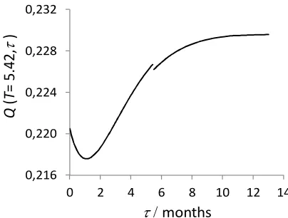
Figure 1: Cost function corresponding to model 2, Q(T*=5.42, t), for M=5, a=10, c=8,
a=0, b=0.1, l=0.3, cp=1, c1=0.025, c0=0.8, ct=1.5, cF=5, cd=500, m2=0.0005. 0,216
0,220 0,224 0,228 0,232
0 2 4 6 8 10 12 14
Q
(T
= 5.42,
t
)
t/ months
Example 1: Time to defect arrival modelled by an exponential distribution
1. External shocks are responsible for defect arrival. The time to the defective state, X, follows an exponential distribution with mean value a. The delay time is assumed to be a Weibull distribution with shape parameter equal to 2 and scale parameter
c.
2. In the base case the mean time to the defective state is a = 10 months. When dealing with model 2 a downtime due to inspection equal to 3.5 hours seems to be a reasonable assumption, therefore we consider that the mean downtime due to inspection is µ2 = 0.0005
3. Cost of preventive replacement,cp = 1 and cost of inspectionc1 = 0.025. In addition
we assume a downtime costs equal to cd= 500
4. The imperfect inspection parameters are α = 0 andβ = 0.1 in the base case.
5. Opportunities occur according to a Poisson process with rateλopportunities per unit of time with λ= 0.3 in the base case.
Figure 1 presents the cost function associated to model 2, that is, when inspections are considered to be non-negligible with an associated downtime cost and when M = 5. In Figure 1, Q(T, τ) is plotted for T =T? = 5.42 and different values of τ. The optimum limit of postponement is τ? = 1.09.
Figure 1 shows the effect on the cost function when the inspection frequency is set at its optimum value and τ varies. Two distinctive features are observed: a discontinuity in τ? = 5.42; and an asymptotic behaviour. The former is due to the indicator function
Ji that points out when the limit of postponement is reached before M T. The latter
reveals that the cost is constant when τ is larger than a particular value, because any of the events, system failure, replacement of the system on opportunity or preventively at
[image:23.612.140.336.308.478.2]M T, will have taken place by that time. Increasing τ does not modify significantly the probabilities of any of the foregoing events.
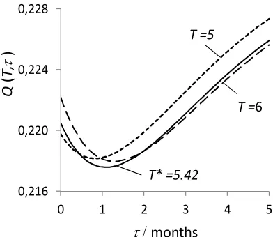
Figure 2: Cost function in model 2, Q(T*=5.42, t) (solid line), Q(T=5, t) (…), Q(T=6, t) (--) 0,216
0,220 0,224 0,228
0 1 2 3 4 5
Q
(T,
t
)
t/ months T =5
T* =5.42
T =6
Figure 2 shows the cost function for three different inspection frequencies. In the three cases the probability of false negative is β = 0.1 and there exists a postponement interval (τ >0) that is preferable to immediate replacement following a positive inspection (τ = 0).
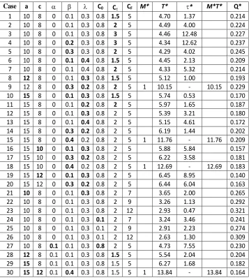
Table 1 shows the optimum policy (M?, T?, τ?) for model 2 for a number of cases. As defects arrive according to a Poisson process the optimum number of inspections is
M? =∞ whenever the probability of false negative is below a threshold. For those cases
preventive replacement. However when the inspection procedure is not reliable, with a high rate of false negatives, the best policy is pure preventive replacement, M? = 1. This result agrees with that in Berrade et al [6] and the study given therein about the consequences of low quality inspections on the optimum policy.
Case a c a b l C0 Ct CF M* T* t* M*T* Q*
[image:24.612.132.489.194.595.2]1 10 8 0 0.1 0.3 0.8 1.5 5 ∞ 4.70 1.37 ∞ 0.214 2 10 8 0 0.1 0.3 0.8 2 5 ∞ 4.49 4.00 ∞ 0.224 3 10 8 0 0.1 0.3 0.8 3 5 ∞ 4.46 12.48 ∞ 0.227 4 10 8 0 0.2 0.3 0.8 3 5 ∞ 4.34 12.62 ∞ 0.237 5 10 8 0 0.3 0.3 0.8 2 5 ∞ 4.29 4.02 ∞ 0.245 6 10 8 0 0.1 0.4 0.8 1.5 5 ∞ 4.45 2.13 ∞ 0.209 7 10 8 0 0.1 0.4 0.8 2 5 ∞ 4.33 5.32 ∞ 0.214 8 12 8 0 0.1 0.3 0.8 1.5 5 ∞ 5.12 1.00 ∞ 0.193 9 12 8 0 0.3 0.2 0.8 2 5 1 10.15 - 10.15 0.229 10 15 8 0 0.1 0.3 0.8 1.5 5 ∞ 5.74 0.53 ∞ 0.170 11 15 8 0 0.1 0.2 0.8 2 5 ∞ 5.97 1.65 ∞ 0.187 12 15 8 0 0.1 0.3 0.8 2 5 ∞ 5.39 3.21 ∞ 0.180 13 15 8 0 0.1 0.4 0.8 2 5 ∞ 5.15 4.61 ∞ 0.172 14 15 8 0 0.3 0.2 0.8 2 5 ∞ 6.19 1.44 ∞ 0.202 15 15 8 0 0.4 0.2 0.8 2 5 1 11.76 - 11.76 0.209 16 15 10 0 0.1 0.3 0.8 2 5 ∞ 5.88 5.84 ∞ 0.157 17 15 10 0 0.3 0.2 0.8 2 5 ∞ 6.22 3.58 ∞ 0.181 18 15 10 0 0.4 0.2 0.8 2 5 1 12.69 - 12.69 0.183 19 15 12 0 0.1 0.3 0.8 2 5 ∞ 6.45 8.95 ∞ 0.140 20 15 12 0 0.3 0.2 0.8 2 5 ∞ 6.44 6.04 ∞ 0.163 21 10 8 0 0.1 0.3 0.8 2 7 ∞ 3.65 2.00 ∞ 0.265 22 10 8 0 0.1 0.3 0.8 2 9 ∞ 3.26 1.13 ∞ 0.292 23 10 8 0 0.1 0.3 0.8 2 12 ∞ 2.93 0.47 ∞ 0.321 24 10 8 0 0.1 0.3 0.1 2 7 ∞ 3.24 3.46 ∞ 0.241 25 10 8 0 0.1 0.3 0.1 2 9 ∞ 2.91 2.23 ∞ 0.274 26 10 8 0 0.1 0.3 0.1 2 12 ∞ 2.63 1.30 ∞ 0.309 27 10 8 0.1 0.1 0.3 0.8 2 5 ∞ 4.73 7.55 ∞ 0.230 28 12 8 0.1 0.1 0.3 0.8 1.5 5 ∞ 5.54 2.04 ∞ 0.204 29 15 8 0.1 0.1 0.3 0.8 1.5 5 ∞ 6.27 1.68 ∞ 0.182 30 15 12 0.1 0.4 0.3 0.8 1.5 5 1 13.84 - 13.84 0.164
Table 1: optimum policy, (M*, T*, t*), and optimum cost, Q*, under different parameter values.
the inspection frequency is robust against changes incτ. Whenλ increases so do both the
inspection frequency and the optimum limit of postponement, albeit τ? experiences the most important change when there is a significant increase in λ. An increasing chance of replacement at an opportunity arising after a true positive can be the reason for both.
When the cost of replacement on opportunity (co) is reduced, so does the inspection
interval, whereas the limit of postponement is extended. As before, the smaller is T?, the higher is the chance of triggering replacement. Extending the limit of postponement (larger τ?) increases the probability of a low-cost replacement at an opportunity.
Not only can a high rate of false negatives make postponement cost-inefficient. When the cost derived from a failure (cF) is high, then both T? and τ? decrease. With more
frequent inspection the maintainer is more aware of defect arrival, increasing both the chance to detect one when it occurs and the chance of replacement on opportunity since a positive inspection triggers the wait for an opportunity. The reduction in τ? makes a
failure less likely to occur.
When the time to the defective state increases (in mean), inspection is relaxed but the postponement time is shortened. This is because a longer time interval between inspections makes it more likely that the unit remains in the defective state until the defect is detected. A shorter τ? is recommended to counterbalance this risk. Concerning the delay time, when this increases both T? and τ? also increase. An increase in the
delay time means that the unit is robust and can function for a longer period. Thus the maintainer can be less attentive to the unit.
In the introduction it was conjectured that imperfect inspections with false alarms may justify postponement. According to the results in Table 1, this conjecture is supported, and thus τ? increases when α increases, and at the same time, the inspection frequency is reduced as the maintainer is less confident about the efficacy of inspection.
Example 2: Time to defect arrival modelled by a Weibull distribution
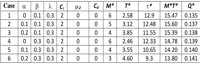
Table 2 shows the optimum policy when the time to defect arrival is assumed to follow a Weibull distribution with shape and scale parameters equal to 2 and 15 respectively. The delay time follows an exponential distribution with mean value equal to 10. The rest of the parameters are: λ = 0.3, cp = 1, c1 = 0.025, co = 0.8, cτ = 2, cF = 5, cd = 0,
Case a b l Ct m2 Cd M* T* t* M*T* Q*
1 0 0.1 0.3 2 0 0 6 2.58 12.9 15.47 0.135
2 0.1 0.1 0.3 2 0 0 5 3.12 12.48 15.60 0.137
3 0.2 0.1 0.3 2 0 0 4 3.85 11.55 15.39 0.138
4 0 0.3 0.3 2 0 0 6 2.46 12.33 14.78 0.139
5 0.1 0.3 0.3 2 0 0 4 3.55 10.65 14.20 0.140
[image:26.612.131.466.126.234.2]6 0.2 0.3 0.3 2 0 0 3 4.60 9.3 13.80 0.141
Table 2: optimum policy (M*, T*, t*) and optimum cost, Q*, under model without
downtime.
The main difference with respect to the previous example is that now the preventive replacement at M T is a preferable choice, instead of replacement at the limit for post-ponement, since τ? > (M? −1)T?. The unit is more prone to enter the defective state as it ages since the memoryless property does not apply. The behaviour of the policy concerning changes in α or β is as before, although now it can be observed that a higher probability of false negatives shortens the time to preventive replacement at M T. In so doing the maintainer gains protection against non-detected defects that in turn lead to failure.
Example 3: Comparison of policies with and without postponement (τ = 0)
with
postponement
without postponement
Case a c l C0 Ct CF M* T* t* Q* M0 T0 Q0
1 10 8 0.3 0.8 1.5 5 ∞ 4.94 1.35 0.204 ∞ 5.81 0.207 2 10 8 0.3 0.8 2 5 ∞ 4.67 3.97 0.215 ∞ 6.82 0.238 3 10 8 0.3 0.8 3 5 ∞ 4.63 12.33 0.218 1 9.23 0.245 4 10 8 0.2 0.8 1.5 5 ∞ 5.48 0.43 0.207 ∞ 5.81 0.207 5 10 8 0.2 0.8 2 5 ∞ 5.04 2.59 0.227 ∞ 6.82 0.238 6 10 8 0.3 0.8 1.5 8 ∞ 4.18 0.06 0.237 ∞ 4.23 0.237 7 10 8 0.3 0.8 4 8 ∞ 3.46 8.51 0.293 1 6.86 0.308 8 10 8 0.3 0.8 2 15 ∞ 3.15 0.05 0.318 ∞ 3.19 0.318 9 10 8 0.3 0.8 3 32 ∞ 2.33 0.04 0.461 ∞ 2.36 0.461
Table 3: comparison of policies with and without postponement (t=0).
[image:26.612.129.493.417.609.2]delayed maintenance with standard policies in order to analyze their respective advantages and disadvantages. This example presents a similar comparison between the model with postponement (τ > 0) and the model without postponement (τ = 0), which is given in subsection 3.1. Here T0, M0 and Q0 will denote, respectively, the optimum inspection
interval, the optimum maximum number of inspections and the optimum cost in the latter case. Further X follows an exponential distribution with mean value a = 10, Y follows a Weibull distribution with shape parameter 2 and scale parameter c = 8. The other parameters are: µ2 = 0.0005, cp = 1, c1 = 0.025, cd = 500. Also, we assume perfect
inspections, that is, α=β = 0.
Cases 3 and 7 in Table 3 indicate that when cτ is comparable with cF (cF/cτ ≤ 2)
postponement is advantageous provided thatcτ is the cost of immediate replacement after
a positive inspection in the policy without postponement. In these cases the immediate replacement is cost-prohibitive and this makes preventive replacement atM = 1 the best option when τ = 0. When case 1 is compared with case 7 and case 4 with case 1 it is observed that the differences between the two policies are reduced if cτ or the rate of
opportunities, λ, decrease. However, the most notable feature is observed for very high values of cF (cases 8 and 9). Then, τ tends to zero and T? ' T0. That is, when the cost
of failure is very large and when the maintainer is confident that the inspection procedure is free or errors, postponement may no longer be an advantageous policy.
5
Conclusions
This paper presents a model to consider the postponement of replacement of a system when it is found to be in a defective state. The model, based on the delay-time concept, assumes that the system can function while it is defective. Thus postponement of re-placement can extend its useful life and reduce rere-placement cost. An opportunity-based replacement is also assumed in addition to the scheduled preventive replacement. We present the analysis of results studying the effect of changes in the model parameters. The results show that the policy is cost-effective provided that the maintainer can rely on the inspection procedure, the rate of opportunities is high enough, and the cost of failure is not too high. Both the time to the defective state and the delay time also play a central role in determining the time limit for postponement. High rates of false negatives lead to a more conservative policy, relying on the scheduled preventive replacement rather than postponement. Nevertheless when α increases the situation is reversed, extending
cost, the study of the consequences of postponement on the system reliability constitute a further, pending issue that can be developed.
The examples reveal that the role of preventive replacement depends on the nature of the time to defect arrival. When the time to defect arrival follows a Weibull distribution the preventive replacement at M?T? is finite in most cases, because the rate of defects
leading to subsequent failure increases as the unit ages. On the contrary when the time to defect arrival is exponential and the probability of an undetected defect is low there is no reason for the preventive replacement at M?T?. If so, the unit is replaced at the limit of
postponement. However a high value of β (false negative) makes preventive replacement preferable to postponement.
When comparing the policies, with and without postponement, the results show that when the cost of failure is large and inspection is perfect τ tends to zero and both the optimum policy and cost-rate converge to those in the policy with no postponement.
Acknowledgments
The work of M.D. Berrade has been supported by the Spanish Ministry of Economy and Competitiveness under Project MTM2015-63978-P. The work of Cristiano A.V. Caval-cante has been supported by CNPq (Brazilian Research Council). M.D. Berrade thanks Dr. Esteban Calvo from the Department of Fluid Mechanics at the University of Zaragoza for his valuable help. The authors acknowledge the comments of the anonymous reviewers for their helpful comments.
References
[1] Adkins, R., Paxson, D. (2013). Deterministic models for premature and postponed replacement. Omega, 41, 1008–1019.
[2] Ascher, H., Feingold, H. (1984). Repairable systems reliability. In: Lecture Notes in Statistics 7, Marcel Dekker, New York.
[4] Bedford, T.; Alkali, B. M. (2009). Competing risks and opportunistic informative maintenance. Proceedings of the Institution of Mechanical Engineers Part O-Journal of Risk and Reliability, 223, 363-372.
[5] Bedford, T.; Dewan, I.; Meilijson, I.; Zitrou, A. (2011). The signal model: A model for competing risks of opportunistic maintenance. European Journal of Operational Research, 214, 665-673.
[6] Berrade, M.D.; Scarf, P.A.; Cavalcante, C.A.V. (2015). Some insights into the effect of maintenance quality for a Protection System IEEE Transactions on Reliability, 64, 661–672.
[7] Berrade, M.D.; Scarf, P.A.; Cavalcante, C.A.V.; Dwight, R.A. (2013). Imperfect inspection and replacement of a system with a defective state: A cost and reliability analysis. Reliability Engineering and System Safety, 120, 80–87.
[8] Berrade, M.D.; Scarf, P.A.; Cavalcante, C.A.V.(2013). Modelling imperfect inspec-tion over a finite horizon. Reliability Engineering and System Safety, 111, 18–29.
[9] Berrade, M.D.; Cavalcante, C.A.V.; Scarf, P.A.(2012). Maintenance scheduling of a protection system subject to imperfect inspection and replacement . European Jour-nal of OperatioJour-nal Research, 218, 716-725.
[10] Chen, W.J. (2009). Minimizing number of tardy jobs on a single machine subject to periodic maintenance.Omega, 37, 591-599.
[11] Christer, A.H. (1987). Delay-time model of reliability of equipment subject to inspec-tion monitoring. Journal of the Operational Research Society, 38(4), 329–334.
[12] Coolen-Schrijner, P.; Shaw, S.C.; Coolen, F.P.A. (2009). Opportunity-based age re-placement with a one-cycle criterion. Journal of the Operational Research Society, 60, 1428-1438.
[13] Dekker, R.; Smeitink, E. (1991). Opportunity based block replacement. European Journal of Operational Research, 53, 46-63.
[14] Dekker, R.; Dijkstra. M. (1992). Opportunity based age replacement: exponentially distributed times between opportunities. Naval Research Logistics, 39, 175–190.
[16] Hau, W.R.; Jiang, Z.H. (2013). An opportunistic maintenance policy of multi-unit series production system with consideration of imperfect maintenance.Applied math-ematics & Information Sciences, 7, 283–290.
[17] Iskandar, B.; Sandoh, H. (2000). An extended opportunity-based age replacement policy. RAIRO Operations Research, 34, 145-154.
[18] Jhang, J.; Sheu, S. (1999). Opportunity-based age replacement policy with minimal repair. Reliability Engineering and System Safety, 64, 339-344.
[19] Koochaki, J.; Bokhorst, J.A.C.; Wortmann, H.; Klingenberg, W. (2012). Condition based maintenance in the context of opportunistic maintenance. International Jour-nal of Production Research, 50, 6918-6929.
[20] Laggoune, R.; Chateauneuf, A.; Aissani, D. (2009). Opportunistic policy for optimal preventive maintenance of a multi-component system in continuous operating units.
Computers & Chemical Engineering, 33, 1499-1510.
[21] Laggoune, R.; Chateauneuf, A.; Aissani, D. (2010). Impact of few failure data on the opportunistic replacement policy for multi-component systems.Reliability Engineer-ing and System safety, 95, 108-119.
[22] Nakagawa,T. (1986). Modified discrete preventive maintenance policies. Naval Re-search Logistics Quartely, 33, 713–715.
[23] Nakagawa, T. (2014). Random Maintenance Policies, Springer, New York
[24] Nakagawa,T., Mizutani, S. (2009). A summary of maintenance policies for a finite interval. Reliability Engineering and System safety, 94, 89–96.
[25] Nakagawa, T., Zhao, X. (2015). Maintenance overtime policies in reliability theory. Models with random working cycles, Springer
[26] Okamura, H.; Dohi, T. (2013). Optimal trigger time of software rejuvenation under probabilistic opportunities.IEICE Transactions on Informations and Systems, E96D, 1933-1940.
[27] Rao, A.N.; Bhadury, B. (2000). Opportunistic maintenance of multi-equipment sys-tem: A case study. Quality and Reliability Engineering International, 16, 487–500.
[29] Satow, T.; Osaki, S. (2003). Opportunity-based age replacement with different in-tensity rates. Mathematical and Computer Modelling, 38, 1419-1426.
[30] Scarf P.A., Cavalcante C., Dwight R., Gordon P. (2009). An age based inspection and replacement policy for heterogeneous components. IEEE Transactions on Reliability
58, 641-648.
[31] Scarf P.A., Cavalcante C. (2012). Modelling quality in replacement and inspection maintenance. International Journal of Production Engineering 135, 372-381.
[32] Taghipour, S., Banjevic, D. (2012). Optimum inspection interval for a system under periodic and opportunistic inspections.IIE Transactions, 44, 932-948. Available from: http://www.tandfonline.com/doi/full/10.1080/0740817X.2011.618176
[33] Taghipour, S., Banjevic, D. (2012). Optimal inspection of a complex system sub-ject to periodic and opportunistic inspections and preventive replacements.European Journal of Operational Research, 220, 649-660.
[34] Tambe, P.P.; Mohite, S.; Kulkarni, M.S. (2013). Optimisation of opportunistic main-tenance of a multi-component system considering the effect of failures on quality and production schedule: A case study.International Journal of Advanced Manufacturing Technology, 69, 1743-1756
[35] van Oosterom, C.D.; Elwany, A.H.; Celebi, D.; van Houtum, G.J. (2014). Optimal policies for a delay time model with postponed replacement. European Journal of Operational Research, 232, 186–197.
[36] Venkat, D.; Coolen, F. P. A.; Coolen-Schrijner, P. (2010). Extended opportunity-based age replacement with a one-cycle criterion. Proceedings of the Institution of Mechanical Engineers Part O-Journal of Risk and Reliability, 224, 55–62.
[37] Vu, H.C., Do P., Barros A., B´erenguer C. (2014) Maintenance grouping strategy for multi-component systems with dynamic contexts.Reliability Engineering and System Safety, 132, 233-249.
[38] Xia, T., Jin, X., Xi, L. , Ni J. (2015) Production-driven opportunistic maintenance for batch production based on MAM-APB scheduling.European Journal of Operational Research, 240, 781-790.
[39] Yang, L. Maa, X., Zhai, Q. and Zhao, Y. (2016). A delay time model for a mission-based system subject to periodic and random inspection and postponed replacement.
[40] Zhao, X., Mizutani, S., Nakagawa, T. (2015). Which is better for replacement poli-cies with continuous or discrete scheduled times? European Journal of Operational Research, 242, 477-486.
[41] Zhao, X., Nakagawa, T. (2016). Over-time and over-level replacement policies with random working cycles. Annals of Operations Research, 244, 103-116.
[42] Zequeira, R.I.; Valdes, J.E.; Berenguer, C. (2008). Optimal buffer inventory and opportunistic preventive maintenance under random production capacity availability.
International Journal of Production Economics, 111, 686-696