Thermal Modeling & Analysis of Carbide Tool Using Finite Element Method

(1)

International Journal of Emerging Technology and Advanced Engineering

Website: www.ijetae.com (ISSN 2250-2459, ISO 9001:2008 Certified Journal, Volume 7, Issue 11, November 2017)

447

Thermal Modeling & Analysis of Carbide Tool

Using Finite Element Method

B.Srinu1, Shankarlinga B S2,Avinash Y K3

1,2,3

Asst. Prof., Dept. of Mechanical Engg, CMR Engineering College, Hyderabad, India

Abstract: The problem of tool wear monitoring in machining operations, has been an active area of research for quite a long time. The accurate prediction of tool wear is important to have a better product quality and dimensional accuracy. In cutting tools the area close to the tool tip is the most important region and conditions at the tool tip must be carefully examined, if improvements in tool performance are to be achieved. The present work involves the study of tool wear caused by the change in hardness of single point cutting tool for a turning operation to predict the tool life in orthogonal cutting based on the heat transfer analysis using Finite Element Method (FEM). The Experiments were performed with EN-24 steel as work piece and Carbide uncoated tool bit as a tool material and the flank wear has been measured experimentally. An empirical relation is used to determine temperature at tool-tip and further Finite Element Method is used to determine the distribution of temperature over the surface of tool and its impact on hardness which is related by an empirical relations. Keywords: Tool wear, FEM, Empirical relation, EN-24 Steel

1. INTRODUCTION

Tool wear monitoring/sensing should be one of the primary objectives in order to produce the required end products in an automated industry so that a new tool may be introduced at the instant at which the existing tool has

worn out, thus preventing any hazards occurring to the machine or deterioration of the surface finish. Cutting tools may fail due to the plastic deformation, mechanical breakage, cutting edge blunting, and tool brittle fracture or due to the rise in the interface temperatures.

1.1 TOOL WEAR

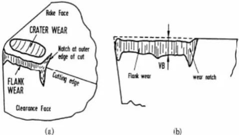
[image:1.595.332.572.606.742.2]

Cutting tools are subjected to an extremely severe rubbing process. They are in metal to metal contact, between the chip and work piece, under conditions of very high stress at high temperature. The situation is further aggravated due to the existence of extreme stress and temperature gradients near the surface of the tool. During cutting, cutting tools remove the material from the component to achieve the required shape, dimension and finish.

(2)

448

1.2 EFFECTS OF TOOL WEAR ON TECHNOLOGICAL PERFORMANCE

• Decrease the dimension accuracy; • Increase the surface roughness; • Increase the cutting force; • Increase the temperature; • Likely cause vibration; • Increase the cost.

1.3 THERMAL ANALYSIS:

In machining operations, mechanical work is converted to heat through the plastic deformation involved in chip formation and through friction between the tool and work piece. Some of this heat conducts into cutting tool, resulting in high tool temperatures near cutting edge.

Experiment Retrospection: Many

experimental methods have been devised to measure the tool, chip or work piece temperature and their distribution, these are:

• Tool-Chip Thermocouple Technique • Embedded Thermocouple Technique • Infrared Radiation Technique

• Metal Microstructure and Micro-hardness Variation Measurement

2. INSTRUMENTATION AND

EXPERIMENTATION

The objective of the present work is to develop methodology to relate tool wear with mechanical properties of a material such as Hardness. Here hardness is related with the modified temperature, including the effect of strain rate, of cutting tool. Finite Element Analysis is used to depict the temperature at various points of cutting tool by changing various machining parameters such as cutting speed (V), depth of cut (d), feed rate (f).

2.1 INSTRUMENTATION

The various instruments used for

experimentation are discussed here in this section:

FORCE MEASUREMENT

A force measurement actually involves the measurement of a deflection, caused by that force, with a suitable calibration between the force and the deflection it produces. For measuring small deflections, various devices have been used. Some of them are listed below:

1. The dial indicator. 2. Pneumatic devices. 3. Optical devices. 4. Piezoelectric crystals. 5. Strain Gauges.

Out of these, most widely used dynamometer is of strain gauge type. In this category, bounded- wire strain gauges have commonly been used. Usually these bonded wire gauges have been specified by the resistance and the gauge factor (F). The gauge factor is a measure of sensitivity of gauge and is defined as:

Where, ∈ is the normal strain and can be

calculated as:

(3)

449

[image:3.595.333.549.295.355.2]

Fig 2.1: Wheatstone bridge (Image Source: www.Google.co.in)

[image:3.595.64.218.361.439.2]

A two component cutting force dynamometer of cantilever type is used in the present work. The dynamometer structure is made of aluminum. The action of the forces is to bend the structure. The axial cutting force, Fc, bends the structure about the one axis and the tangential feed force, Ff, bends the structure about another axis.

Fig 2.2: Dynamometer (Image Source: www.Google.co.in)

2.2 EXPERIMENTATION

Experiments were carried out on a turning lathe. A carbide tip turning tool was clamped in a two component strain gauge dynamometer using a tool holder designed in a machine lab

during the thesis work. For the

experimentation, EN 24 steel work piece of 600mm length was held in a three – jaw chuck and supported by a center in the tail stock.

The experiments were made on the HMT lathe using a bar turning process under dry conditions. For the range of range of cutting conditions (cutting speed, feed, and depth of cut) it was required to measure the two force components Ft and Ff, thickness of chip and flank wear. A total of eight experiments were carried out, all with the same basic configuration and carbide inserts were

replaced after performing a single test so as to see the effect of temperature on the tool individually at different cutting conditions. The selected ranges of each parameter used are given below:

• Work material: The EN 24 Steel (0.35- 0.45 %C, 0.45- 0.6 %Mn, 1.3 - 1.8 %Ni) was chosen for the present investigation with a diameter of 60 mm and 600mm length.

The figure 3.3 shows the dimensions of the work piece (EN24) before the turning process.

• Tool material: The tool material used should be capable of high speed machining with dry cutting conditions. In present investigation carbide inserts were used for performing the experiments.

• Tool geometries:

a) Tool length: 16.02mm b) Tool width: 8.02 mm c) Nose radius: 0.4 mm

• Test conditions: carbide inserts were used to machine EN24 steel with following cutting parameters

a) Rotational speed:70.08 – 179.82 (m/min) b) Feed: 0.0787 – 0.175 (m/sec)

c) Depth of cut: 0.508,0.762,127 (mm)

[image:3.595.333.542.668.734.2]

(4)

450

Then the actual experiments have been carried out with the different input cutting conditions for different experiments for constant volume of material removal in each case. The

experiments carried out can be classified:

1. Carry out experiment on lathe machine using EN 24 as work piece and commercial available Carbide Tool of triangular shape.

2. Machining is done with different sets of Cutting speed, depth of cut, & feed rates.

3. Measuring the cutting forces with

dynamometer.

3.ANALYSIS

The present chapter deals with the formulation of three-dimensional governing equation for heat conduction used to obtain the temperature distribution on the face of the tool bit, to be used for obtaining the hardness at the various positions on the tool. The eight noded brick elements have been used for the FEM modeling.

3.1 GOVERNING EQUATION FOR THE HEAT TRANSFER

Governing equation for the heat transfer problem can be written as:

Following assumptions have been considered for the simplicity if the computation required:

1. Conduction occurs in the steady state,

2. Material is isotropic and homogeneous as (Kx = Ky = Kz = K)

3. Internal heat generation is zero.

3.2 BOUNDARY CONDITION

Following boundary conditions have been used for the solution of the present problem:

1. Temperature is specified at nodes which are in touch with shear zone [1], [4], [20], and [22], and

∆y = spacing between successive planes (25 *10-4 mm) ∆y = spacing between successive planes (25 *10-4 mm)

2. Convection is taking place on surface from

the tool bit to air, taking

Where, T ∞ = 27 ο C

3.3 FEM FORMULATION

To achieve the close boundary

(5)

451

coordinate system into distorted shapes in global Cartesian system and then evaluating the element equation for the distorted element. The parent element may be selected from lagrangian / serendipity family. The Local Coordinate System associated with parent

element is called curvilinear coordinate. The

Serendipity coordinates for elements are represented as:

Here, nc = Total number of nodes per element and for isoperimetric elements, Mi = Ni

Now to evaluate the B–matrix we need to evaluate the derivative of shape function with respect to x, y and z. The derivative cannot be found out directly as shape function is expressed in terms of natural coordinates (ξ, η, ζ). So by using chain rule differentiation

The above equation can be further written in the form as given below [K]{T}= {Q}

Where [K] = Thermal conductance coefficients matrix

{T}= Nodal temperature vector.

{Q}= Nodal heat flux or heat load vector.

3.4 HARDNESS OF TOOL

Since effects of temperature are being considered on flank wear, so it becomes necessary to consider thermal softening of cutting tool material. Relationship between temperature and thermal softening.

(6)

452

[image:6.595.84.294.158.575.2]

3.5 SOLUTION SCHEME

Fig 3.1: Solution Flow Chart.

4. RESULTS AND DISCUSSIONS

In the present chapter the results for the present problem, that is for the solution of the thermal softening of the tool material in order to predict the tool wear have been developed in accordance with the previously developed models for tool wear [4], [20]and [22].

The number of experiments has been conducted to find out the cutting forces and flank wear of the tool, made of tungsten carbide, at varying machining parameters, which are cutting speed (V), cutting feed (f) and depth of cut (d). Using the experimental data, the strain rate and average interface temperature for the various cutting conditions have been obtained, which have been ultimately used to determine the modified temperature at the tool and the work piece contact area.

4.1 MODELLING OF SOLUTION DOMAIN USING FEM

In order to use the finite element technique, mathematical expressions have been derived and discussed in the previous chapter and have been used to predict the temperature at the various locations of the cutting tool. The following are the details of the discrimination of the solution domain carried out for the FEM Analysis and thus used in the developed computer program for the generation of the results. Problem is for: 3 D heat conduction

Type of elements: Eight Noded brick elements (Serendipity family)

Total node: 288 Total elements: 168

Node per element: 8 Node per face: 4

Number of fixed nodes: 3 (temperature at the tip of the cutting tool)

(7)

453

4.2 VARIATION OF HARDNESS WITH FLANK-EDGE DISTANCE

[image:7.595.333.559.271.364.2]

The figure 5.2 shows the relation of tool hardness with the flank distance at different temperature distribution on flank edge of the carbide tool bit. As at the tool tip the temperature is maximum, therefore the hardness is less.. At the same flank-edge distance, for these values of modified cutting temperatures, we have different hardness values along the flank face of the tool. The temperature starts decreasing because of heat loss as we move away from the tool tip along the flank surface the hardness of material increases.

Fig 4.1: Relation between hardness and flank distance

4.3 VARIATION OF TEMPERATURE WITH CUTTING FORCE

Fig 4.2: variation of temperature with the cutting force

The figure 4.2 shows the variation of temperature with the cutting force. As shown in the graph, as the cutting forces increases the temperature at the tip of the cutting tool also

increases due to higher frictional forces at the tip of the carbide tool bit. This increased temperature of the tool leads to the reduction of hardness value of the cutting tool and thus the tool wear.

[image:7.595.85.307.402.498.2]

4.4 VARIATION OF FLANK WEAR WITH CUTTING FORCE

Fig 4.3: variation of the wear with the cutting tool Force

The figure 4.3 shows the variation of the wear with the cutting tool Force. As shown the flank wear of carbide insert increases with the increase in the forces during the bar turning process. This is because increase in forces leads to increase in the temperature of the cutting tool as shown in figure 5.3 and increased temperatures further leads to the flank wear of the cutting tool due to the thermal softening.

4.5 VARIATION OF FLANK WEAR WITH MODIFIED CUTTING TOOL

TEMPERATURE

[image:7.595.70.296.576.669.2]

(8)

[image:8.595.80.300.145.207.2]

454

Fig 4.4: Variation of flank Wear with respect to modified temperature

4.6 VARIATION OF TEMPERATURE WITH CUTTING VELOCITY

Fig 4.5: Relation of cutting velocity versus temperature.

[image:8.595.333.562.181.263.2]

The figure 4.5 shows a relation of cutting velocity versus temperature, at constant feed at different levels depth of cuts used in experimentation work. The inference that can be drawn from the above graph is that when we increase the cutting velocity the temperature keeps on increasing.

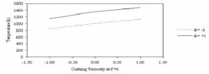
Fig 4.6: Relation of cutting velocity versus temperature.

The figure 4.6 depicts the same trends as figure 4.5, from these trends it’s depicted that with the increase in velocity of cutting, the temperature raises. These two graphs are at constant depth of cuts for each curve. The figure 4.7 shows results of temperature with cutting velocity at constant depth of cuts. It

[image:8.595.70.290.296.384.2]

shows temperature increase with increase in depth of cut.

Fig 4.7: Results of temperature with cutting velocity.

4.7 VARIATION OF FLANK WEAR WITH CUTTING VELOCITY

(FOR CONSTANT FEED RATE)

Fig 4.8: variation of wear with the cutting velocity

Here the results have been shown for the variation of wear with the cutting velocity of the tool. In figure 4.8 trend of cutting velocity with wear has been shown at constant feed of -1, that is the lowest feed taken in experiments at different depth of cuts shows almost same pattern of increasing flank wear with increase in velocity.

4.8 VARIATION OF FLANK WEAR

WITH CUTTING VELOCITY(FOR

CONSTANT DEPTH OF CUTS)

[image:8.595.70.284.550.626.2]

(9)

[image:9.595.78.288.147.219.2]

455

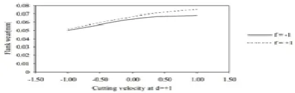
Fig 4.9: variation of wear with the cutting velocity at constant depth of cuts.

Fig 4.10: variation of wear with the cutting velocity at constant depth of cuts.

The figure 4.10 also shows similar results but at depth of cuts (d = +1). The trend is almost same depicted in other graphs as shown before, that is with increase in the cutting velocity for some constant value of depth of cut, the tool wear increases.

5. CONCLUSIONS

Based on the results presented in previous sections, the following conclusions have been observed:

1. The hardness increases with increase in distance from the flank edge and with decrease in the tool-work piece contact temperature.

2. The change in the tool work piece contact

temperature depends upon the cutting

parameters and it increases with increase in resultant cutting force, but do not follow a linear trend and thus we can find an optimum set of machining parameters to have a minimum heat generation at tool-work piece contact.

3. The flank wear is directly proportional to the resultant cutting force and approximately follows a linear trend.

4. The flank wear increases with increase in modified cutting tool temperature (due to increase in the strain rate), but there is a nonlinear trend so we can find an optimum value of cutting parameters so as to give minimum strain rate, because heat generated increases with increase in the strain rate.

5. The contact temperature increases with the increase in the cutting velocity, but at constant cutting velocity, there is a significant increase in the contact temperature with increase in the depth of cut as compared to the increase in the contact temperature with the increase in the feed rate.

5.1 SCOPE FOR FUTURE WORK

With increasing competitiveness as observed in the recent times, manufacturing systems in the industry are being driven more and more aggressively. So there is always need for perpetual improvements. Thus for getting still more accurate results we can take into account few more parameters as given below:

• The transient analysis for the machining operation can be studied.

• The study can also be extended on coated carbide tools, CBN, or other harder tools.

• CNC machines can be used for the experimentation to have the better control of the process variables and also parameters can be set to the desired accuracy.

• The presently developed system can be used

for other conventional as well as

[image:9.595.69.284.273.341.2]

(10)

456

References

[1]. J N Reddy, “An introduction to finite element Method”, McGraw-Hill, 1993.

[2]. B.S Raghuwanshi, “A Course in Workshop Technology”, Dhanpat Rai & Co, Vol-2 (1998). [3]. G.K.Lal, “Introduction to machining science”,

New Age International Publishers, 1999. [4]. R.K.Jain, “Production Technology”, Khanna

Publishers, 2001

[5]. Tirupathi R.Chandrupatla, Ashok D. Belegundu, “Introduction to Finite Elements in Engineering”, Pearson Education, 2002. [6]. Shih Albert J., Yang Henry T.Y.,

“Experimental and Finite Element Predictions of Residual Stresses due to Orthogonal Metal Cutting”, International Journal for Numerical Methods in Engineering, vol. 36(1993), pp.1487-1507.

[7]. Shih Albert J, “Finite Element Simulation of Orthogonal Metal Cutting”, Journal of Engineering for Industry”, ASME, vol. 117(1995), pp. 84-93.

[8]. Gillibrand D., Bradbury S.R., Yazdanpanah, Mobayyen S.,“A Simplified approach to Evaluate the Thermal Behaviour of Surface Engineered Cutting Tools”, Journal of Surface & Coatings Technology, vol. 82(1996), pp.344- 351.

Author’s Profiles:

B. Srinu Completed B.Tech in Mechanical Engg,(2013) at JITS, Warangal, and Master’s Degree in CAD/CAM,(2015) at MEC, Hyderabad. He had 2 years of teaching experience, and presently working as Asst. Prof. at CMR Engineering College, Hyderabad.

Shankarlinga B S Completed B.E degree in Mechanical Engineering (2013) at GEC Raichur, and master degree in Product Design and Manufacturing (2015) at PG center, VTU, Belagavi, He had 2 years of teaching experience. Currently he is working as Asst.Prof, in CMR Engineering College, Hyderabad, India.