WiMAX Traffic Forecasting on Daily basis with Trainable Cascade-Forward Backpropagation Network in Wavelet Domain

(1)

International Journal of Emerging Technology and Advanced Engineering

Website: www.ijetae.com (ISSN 2250-2459,ISO 9001:2008 Certified Journal, Volume 4, Issue 8, August 2014)

152

WiMAX Traffic Forecasting on Daily basis with Trainable

Cascade-Forward Backpropagation Network in Wavelet

Domain

Mankhush Singh

1

, Simarpreet Kaur

2

1_{M.Tech (E.C.E) Student,}2_{Department of E.C.E, Baba Banda Singh Bahadur Engineering College, Fatehgarh Sahib}

Abstract— In this Paper, the WiMAX Traffic Forecasting on Day basis is done. The traffic time series is decomposed with Stationary Wavelet Transform (SWT). Further these coefficients will be trained and predicted with the Trainable Cascade-Forward Backpropagation Neural Networks. The quality of forecasting obtained is shown in terms of the four parameters.

Keywords— MAE, Neural network SWT, RSQ, RMSE, SMAPE, WiMAX.

I. INTRODUCTION

Worldwide Interoperability for Microwave Access (WiMAX) technology is a modern solution for wireless networks. One of the most difficult problems that appears in the WiMAX network is the non uniformity of traffic developed by different base stations. This comportment is induced by the ad hoc nature of wireless networks and concerns the service providers who administrate the network. The amount of traffic through a base station (BS) should not be higher than the capacity of that BS. If the amount of traffic approaches the capacity of the BS, then it saturates. Due to the traffic non-uniformity, different BS will saturate at different future moments. These moments can be predicted using traffic forecasting methodologies.

II. TRADITIONAL APPROACHES

The traditional approaches for time series forecasting assume that time series is issued from linear processes, but it may be totally inappropriate if the underlying mechanism is nonlinear [5]. One of the models is based on Box-Jenkins methodology which is used for building the time series model in a sequence of steps which were repeated till the optimum model is not achieved.

Second class of models used the structural state space methods that are used to predict the stationary, trend, seasonal, and cyclical data. These methods capture the observations as a sum of separate components (such as trend and seasonality). Between all of the above forecasting models, artificial neural networks (ANNs) have been shown to produce better results [3], [4] and [7]. In [10], the performance and the computational complexity of ANNs are compared with the ones obtained using ARIMA and fractional ARIMA (FARIMA) predictors, Wavelet based predictors and ANNs. The results of this study show the significant advantages for the ANN technique. In [6], the advantage of the ANN over traditional rule-based systems is proved. The authors of [8], [11] and [9] propose a time delayed neural network (TDNN). The forecasting accuracy by using Wavelet Transform is described in [2]. The paper presents a forecasting technique for forward energy prices, one day ahead. The results demonstrate that the use of Wavelet Transform as a pre-processing procedure of forecasting data improves the performance of prediction techniques.

III. FORECASTING PROCEDURE

(2)

International Journal of Emerging Technology and Advanced Engineering

153

Input Data

Test Data

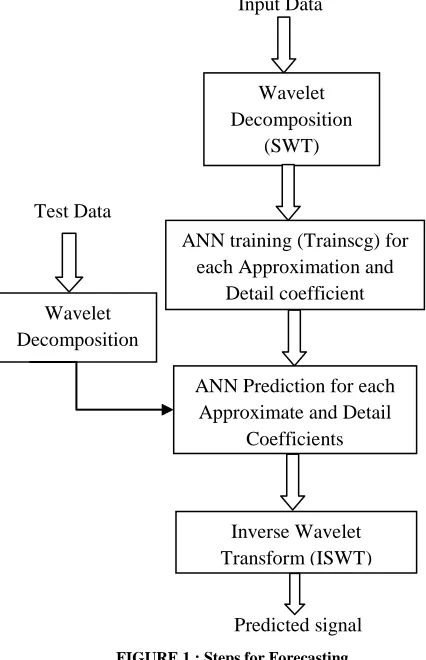
[image:2.612.52.265.139.469.2]

Predicted signal

FIGURE 1 : Steps for Forecasting

1) Using the Haar Wavelet decompose the data for input and testing, with the Stationary Wavelet Transform. 2) Arrange the Approximate and Detailed coefficients

obtained from the each of the Four levels.

3) Establish the trainable cascade-forward

backpropagation networks for each level of the decomposition obtained from the input data.

4) keeping the "tansig" (Hyperbolic tangent sigmoid transfer function) for calculating the layer's output from its network input. Train these networks using "trainscg" (Scaled conjugate gradient backpropagation function) of Matlab.

5) Predict each decomposition level of the forecasted signal using the decomposed signal and the obtained model.

6) Apply Inverse Stationary Wavelet Transform to obtain the final predicted signal.

IV. THE WAVELET TRANSFORM

Wavelets divide the data into several frequency components, then process them at different scales or resolutions. The multi-resolution analysis (MRA) is a signal processing technique that considers the signal's representation of multiple time resolutions. At each temporal resolution two categories of coefficients are obtained: Approximation and Detailed coefficients. Generally the MRA is implemented based upon the algorithm proposed by Stephane Mallat [12], which computes the Discrete Wavelet Transform (DWT). The disadvantage of this algorithm is the decreasing of the sequences length of the coefficient with the increase of the iteration index because of the utilization of the decimators. Another way to implement a MRA is to use Shensa’s algorithm [13] (which corresponds to the computation of the Stationary Wavelet Transform (SWT)). In this case the use of decimators is avoided but at each iteration different low-pass and high-pass filters are used. In this paper we used the SWT with the following purposes:

 To extract the overall trend of the temporal series that describes the traffic under analysis with the aid of the approximation coefficients.

 To extract the variability around the overall trend with the aid of some detail coefficients.

The reconstruction is done through the Inverse Stationary Wavelet Transform (ISWT). In [1], the best mother wavelet used for the prediction accuracy of the traffic variability is the Haar wavelet. So Haar will be used as wavelet for decomposition in SWT by us.

V. ARTIFICIAL NEURAL NETWORKS AND DATA

CONFIGURATION

We used Trainable Cascade-Forward Backpropagation network in our forecasting process. An Artificial Neural Network is a mathematical nonlinear model which is composed of interconnected simple elements, called artificial neurons. An ANN has three characteristics:

1) The architecture of interconnected neural units.

2) The learning or training algorithm for determining the weights of the connections. The training function used in our approach is Trainscg which is a network training function that updates weight and bias values according to the scaled conjugate gradient method.

Wavelet Decomposition

(SWT)

ANN training (Trainscg) for each Approximation and

Detail coefficient

ANN Prediction for each Approximate and Detail

Coefficients

Inverse Wavelet Transform (ISWT) Wavelet

(3)

International Journal of Emerging Technology and Advanced Engineering

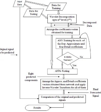
[image:3.612.109.504.144.584.2]

154

FIGURE 2 : Block Diagram of the Trainable Cascade-Forward Backpropagation Neural network modeling

3) The activation function that produces the output based on the input values. And the Transfer Function used here is Tansig which is a neural transfer function that calculates the layer's output from its network input.

Now the first step is to split the data into training and testing data sets. The next step is the MRA pre-processing of both the training and testing data sets. The nth level of decomposition depends upon the length of the input data.

(4)

International Journal of Emerging Technology and Advanced Engineering

155

Giving us the 672 samples for a single week and 5376 samples for the eight weeks. The output signal is compared with the real data and the results are given out in terms of four parameters.

VI. RESULT PARAMETERS

The Forecasting ability of our model is evaluatedin terms of the following well-known evaluation parameters :

 Symmetric Mean Absolute Percent Error

(SMAPE): calculates the symmetric absolute error in percent between the actual traffic X and the forecasted traffic F across all observations t of the test set of size n for each time series s.

the ideal value of SMAPE being 0.

 Mean absolute error (MAE): It represents the average absolute error value. The mean absolute error (MAE) is given by:

 R-Square (RSQ): The coefficient of determination R2, in statistics, is the proportion of variability in a data set that is accounted for by a statistical model. In this definition, the term variability is defined as the sum of squares. A version for its calculation is:

where

The ideal value of RSQ being 1.

In which Xt, Ft are the original data values and modeled

values (predicted) respectively, while Xt and Ft are the

means of the observed data and modeled (predicted) values, respectively. SST is the total sum of squares, SSR is the

regression sum of squares.

 Root Mean Square Error(RMSE): It measures the differences between the values predicted by the model and the values actually observed from the time-series being modeled or estimated.

Where Ft is the prediction and Xt is the true data value.

TABLEI

FORECASTING RESULTS FORDAYPREDICTIONS

Week No. Week 8 Week 7

Day Thursday Friday Saturday

SMAPE 0.3734 0.3523 0.3503

MAE 0.3454 0.3456 0.3191

RSQ 1.1486 1.0902 0.9915

RMSE 1.5396 1.5316 1.4024

TABLEI

CONTINUED...

Week

No. Week 6 Week 5 Week 4

Day Sunday Saturday Wednesday

SMAPE 0.3053 0.3786 0.3510

MAE 0.2955 0.3500 0.3414

RSQ 1.0276 1.0618 1.0123

(5)

International Journal of Emerging Technology and Advanced Engineering

156

0.3734

0.3523 0.3503

0.3053

0.3786

0.351

0 0.1 0.2 0.3 0.4

W8(Thursday) W7(Friday) W7(Saturday) W6(Sunday) W5(Saturday) W4(Wednesday)

SMAPE Values

CHART 1: SMAPE Values for DAY Prediction of the Traffic

0.3454 0.3456

0.3191

0.2955

0.35

0.3414

0.26 0.28 0.3 0.32 0.34 0.36

W8(Thursday W7(Friday) W7(Saturday) W6(Sunday) W5(Saturday) W4(Wednesday)

MAE Values

CHART 2: MAE Values for DAY Prediction of the Traffic

1.1486

1.0902

0.9915

1.0276

1.0618

1.0123

0.9 0.95 1 1.05 1.1 1.15

RSQ Values

(6)

International Journal of Emerging Technology and Advanced Engineering

157

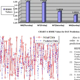
1.5396 _1.5316

1.4024

1.3511

1.5014

1.486

1.25 1.3 1.35 1.4 1.45 1.5 1.55

RMSE Value s

[image:6.612.56.364.167.475.2]

CHART 4: RMSE Values for DAY Prediction of the Traffic

FIGURE 3 : Trends of the Original Data and the Predicted Data

VII. CONCLUSION

In this paper the Haar wavelet decomposition using the Stationary Wavelet Transform gave us the Approximate and Detailed coefficients for four decomposition levels. Then these coefficients were trained by the Trainable Cascade-Forward Backpropagation Neural network for predicting the WiMAX traffic for the single day. It is observed that the SMAPE, MAE, RSQ and RMSE values have improved because of the use of Training Function "Trainscg" of Matlab. The neurons that used the "tansig" transfer function for obtaining the output from the neural network have added for the further improvements. This forecasting technique can also be used for building prediction models for the time series that are present there in our various day to day businesses and rate exchange processes like Stock Exchanges.

Also it would be better to have more data for analysis in order to have higher performance and to reduce the prediction errors.

REFERENCES

[1] Cristina Stolojescu, Ion Railean, Sorin Moga, Alexandru Isar, Comparison of Wavelet Families with Application to WiMAX Traffic Forecasting, 12th International Conference on Optimization of Electrical and Electronic Equipment, OPTIM 2010.

[2] Nguyen, H. T, Nabney, I. T, Combining the Wavelet Transform and Forecasting Models to Predict Gas Forward Prices, ICMLA '08: Proceedings of the 2008 Seventh International Conference on Machine Learning and Applications, IEEE Computer Society, pp. 311-317, 2008.

[3] S. Armstrong, M. Adyaa, An application of rule based forecasting to a situation lacking domain knowledge, International Journal of Forecasting, Vol. 16, pp. 477-484, 2000.

[4] A. Mitra, S. Mitra, Modeling exchange rates using wavelet decomposedgenetic neural networks, Statistical Methodology, vol. 3, issue 2, pp. 103-124, 2006.

[5] G. Zhang, B. E. Patuwo, M. Y. Hu, Forecasting with artificial neural networks: The state of the art, International Journal of Forecasting 14, pp.35-62, 1998.

[6] N. Clarence, W. Tan, Incorporating Artificial Neural Network into a Rulebased Financial Trading System, The First New Zealand International Two Stream Conference on Artificial Neural Networks and Expert Systems (ANNES), University of Otago, Dunedin, New Zealand, November 24-26, 1993.

[7] G. Ibarra-Berastegi, A. Elias, R. Arias, A. Barona, Artificial Neural Networks vs Linear Regression in a F luid Mechanics and Chemical Modeling Problem: Elimination of Hydrogen Sulphide in a Lab-Scale Biojilter, IEEElACS International Conference on Computer Systems and Applications, pp.584-587, 2007.

(7)

International Journal of Emerging Technology and Advanced Engineering

158

[9] G. Peter Zhang, Min Qi, Neural network forecasting for seasonal and trend time series, European Journal of Operational Research 160, pp. 501-514, 2005.

[10] H. Feng, Y. Shu, Study on Network Traffic Prediction Techniques, Proceedings of the International Conference on Wireless Communications, Networking and Mobile Computing, Vol. 2, pp. 1041- 1044, 2005.

[11] Daniel S. Clouse, C. Lee Giles, Bill G. Home, Garrison W. Cottrell, Time-Delay Neural Networks: Representation and Induction of FiniteState Machines, IEEE Transaction on Neural Networks, vol. 8, no. 5, September 1997.

[12] S. Mallat, A Wavelet Tour of Signal Processin, Second Edition, 1999.