Improved Algorithm for Auto-Tuning of PID Controller using Successive Approximation Method

(1)

International Journal of Emerging Technology and Advanced Engineering

Website: www.ijetae.com (ISSN 2250-2459, ISO 9001:2008 Certified Journal, Volume 9, Issue 3, March 2019)

55

Improved Algorithm for Auto-Tuning of PID Controller using

Successive Approximation Method

Gade Sachin Shamkiran

1

, Dr. Sanjay A. Pardeshi

2

1

Research Scholar Shivaji University Kolhapur Maharashtra

2_{Professor, RIT, Islampur, Sakharale}

Abstract— ON line auto tune algorithm of Proportional-Integral-Derivative (PID) controller using successive approximation method is reviewed in this paper. Furthermore, detailed mathematical analysis of PID control equation is formulated for understanding of basic PID controller. The result of mathematical analysis come up with a numerical based tuning method. This new tuning method is the updated or improved tuning method over the existing tuning strategies based on numerical method. Using this new tuning method, PID controller has less overshoot and settling time as compared with its earlier numerical tuning algorithm. Effect of noise on PID parameters during online tuning process is analyzed and suggested method to modify PID parameters. In this present work, settling time is calculated as the function of PID parameters and settling time is correlated with new constant R and R’. MATLAB based simulation results are much more agreed with theoretical analysis of PID controller.

Keywords—PID Controller, Tuning of PID controller, Successive Approximation Method, Online Tuning, PID mathematical analysis.

I. INTRODUCTION

Well-tuned PID controller shows good performance with small overshoot, minimum settling time. The tuning of PID controller is the well-known problem in the research area and many of researchers are working on tuning method of PID controller. PID tuning rules or methods suggested in literature is broadly categorized on the basis of concepts like process dynamics [2.3], analytical tuning method [4], fuzzy rule based tuner [5-10], using hybrid approach [11-13], genetic algorithm [14-16] and optimization algorithm [17]. But, it is found that there are only a small number of literatures suggested online auto tuning of PID controller [18-25]. Most of the process industries try to tune their system online. There are only few tuning methods those are based on numerical method [26, 27].

In this paper, in-depth analysis of Successive Approximation Method (SAM), PID tuning rules have been considered which are to be considered as foremost rules ended [26, 27]. The analysis is carried out for settling time and effect of noise on PID parameters.

This will help more for theoretical design of PID controller. Supplementary to the previous rule of SAM new improved algorithm is discussed with noise correction technique and this showed good performance as compared with its earlier algorithm. New constants R, R‘ and settling time has found correlation and consecutively this is suitable for determination of PID parameters under constrained conditions.

II. TRADITIONAL PID CONTROLLER

In 1922, Nicholas Minorsky was first who proposed Traditional PID controller for automatic steering of ships [1]. The equation of motion and class of control equations are as follows

(1)

(2)

(3)

(4)

Equation 1 is representing equation of motion and equation 2, 3 and 4 are the first, second and third order of class of control. Integrating equation 3 then,

∫ (5)

Integral term = ∫

Proportional term =

Derivative term =

Condition for stability is,

( ) (6)

P is the state of process dynamics that closely related with the derivative gain of PID controller. The modular parallel non-interacting form of PID controller is,

(2)

International Journal of Emerging Technology and Advanced Engineering

56

This is well known PID controller equation and computer implementation of the PID equation is possible using a numerical method. Numerical differentiation and integration after simplification is given as,

*∑ ( )

_(∑ _{( )}

( ) ( )

)

+ (8)

∫ [( ) ∑ ∑ ( )](9)

Where e is error (e) =set point (SP) – process value (PV) Assume, h = 1 unit sample time. At e=0 from equation 7

∫ (10)

III. AUTO TUNING USING SUCCESSIVE APPROXIMATION

METHOD

Online auto-tuning of PID controller using Successive Approximation Method provides following tuning rules while other parameters momentarily equating to zero [26,27].

(11)

(12)

(13)

Assume real roots only then the solution of differential equation 7 is,

(14)

Where C_1 and C_2 are constants and calculated by using initial and steady state condition and r_1, r_2 given as,

√

(15)

√ (16)

Software model for tuning mode of PID controller is mentioned in [26] as follows,

This equation can be written as,

(17)

Assume real roots only then the solution of differential equation 17 is as follows,

(18)

Integrating equation 7 and Assume real roots only then the solution of this equation is as follows,

(19)

Equation 14 and 18 are the indirect solution of equation 2 and 3 respectively and equation 19 is the solution of integral of equation 2. Thus in other word equation 14, 18 and 19 are the solution of three different class of control.

1 SETTLING TIME

Assume at steady state the error tends to 0 and constants from the equation 14, 18 and 19 are fitted such that in the said equation this to satisfy the constraints by assuming approximate curve fitting, since from a mathematical point of view there is no change in the value of constant when either differentiating or integrating particular equation. (Derivative of constant is zero.) Hence note down as,

and (valid only under

asymptotic approximation when steady-state error tends to zero) and equating remaining terms as follows,

(20)

Consider three set as,

(21)

(22)

(23)

Solving differential equation 21 and 22 for ‗t‘ which is nothing but settling time of PID controller as error approaches zero. Solutions are as follows,

₍₂₄₎

(3)

International Journal of Emerging Technology and Advanced Engineering

57

(26)

For the simplicity, let consider as,

(27)

₍₂₈₎

Differentiating equation 28 w.r.t. ‗R‘ and after simplification is given as,

(

( )

) ( ) (29)

Similarly, the following expression can be derived,

(30)

₍₃₁₎

Differentiating equation 31 w.r.t. R' and after simplification is given as,

(

( )

) ( ) (32)

Settling time by the equation 28, 29, 31 and 32 is R and R' dependent.

IV. IMPROVED TUNING METHOD

Equation number 18, 14 and 19 are the solution of dy/dt,

y, ∫ respectively. The solution of each is recursive

function as examined equations with the constant parameter

as a weighting factor. Reciprocal of these parameters Ki,

KP, KD is the weighting factor of equation 18, 14, and 19

respectively. Tuning rules can be formulated using equation 7, 17 and integral form of equation 7 according to the method suggested in [26, 27] as follows,

factor= (33)

∫ factor= (34)

∫ ∫ ∫ factor= (35)

Notice that for all class of control equations derived as

like dy/dt , y, ∫ these are all special cases of each

other having same PID constants. Ki, KP, KD are the PID

parameters and those are constants, hence PID parameters calculated using equation 33, 34 and 35 should be same.

Integral action is responsible for the sum of error throughout time interval up to only settling time and after settling time integral action should be replaced by ‗u‘ so that the saturation limit for integral action is inserted. Suppose noise is added in each error signal then the integral action also provides the sum of noise present in error signal. Thus the integral action provides the sum of error as well as the sum of noise.

Derivative action provides the rate of change of error and this action is more sensitive to noise. Suppose noise is added to each error signal then the derivative action provides rate of change of error with noise and the added error can have brought out a common factor of derivative action and if divided by this factor to derivative constant noise will cancel out from this term and hence for auto-tuning using successive approximation method uses derivative form instead of integral form because noise can be canceled out by multiplying suitable correction factor to the PID constants. Equation 33 is selected for the tuning of PID parameters and these are well-known rules of successive approximation method. Equation 7 is used after the tuning process is completed for normal mode.

PID constants are calculated with the assumption that momentarily other PID parameters equating to zero and hence some error lies in the tuning parameters. This hypothesis is assumed for the simplicity of present algorithm but to the correct form of tuning equations, the precise form of tuning rules can be provided assuming that all PID constants are present when calculating PID parameters during auto tuning mode. The sequence of parameter calculations are as follows and one should stick up with this sequence. The improved tuning rules for successive approximation method is as follows,

( ) ₍₃₆₎

( )

(37)

( ) (38)

V. CORRECTION DUE TO NOISE AND CONVERGENCE

(4)

International Journal of Emerging Technology and Advanced Engineering

58

Noise filtering method can be inserted during updating of PID constants during auto-tune mode. If the averaging method is used then updating equations will be given as,

₍₃₉₎

The adaptive filter may be suggested at this stage to cancel out the noise and correcting PID constants at a great level of accuracy. The correction factor is calculated which is based on the root locus of equation 15 and 16.

Consider 36, 37 and 38 to be tested for convergence, when output is bounded and provide finite results for finite and bounded inputs, there should upper and lower bounds. Hence, PID parameters are bounded as follows,

Let consider that,

Plant output limits (40)

If plant output is bounded then the error shall be within the limit as,

Error limits (41)

As the error is limited then PID parameters are bounded as,

Proportional (42)

Integral (43)

Derivative (44)

Iteration loop is terminated if,

| |

(45)

| |

(46)

| |

(47)

Where these are the predefined allowable

absolute relative error values. If the condition in equation 45, 46, 47 is satisfied then the tuning process will be terminated.

VI. ILLUSTRATIVE EXAMPLE

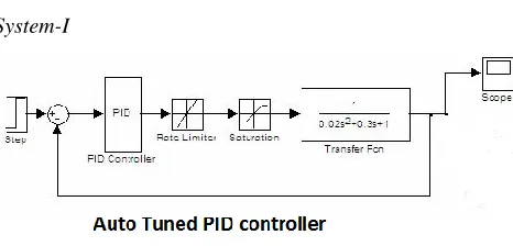
[image:4.612.327.560.145.257.2]

System-I

Figure 1: SAM PID MATLAB model

MATLAB Simulink model (Fig. 1) is developed to simulate improved SAM PID controller with a system suitable for illustration purpose. Consider second order simple plant/system with following transfer function as

( ) (40)

Auto tuning of said system is carried out using three different algorithms which are listed below,

1. Auto-tuning using SAM PID method. (equation 33)

(Method 1)

2. Auto-tuning using improved SAM PID method

(equation 36, 37 and 38) (Method 2)

3. Auto-tuning using improved SAM PID method with

noise correction suggested in section 5 and 6. (Method 3)

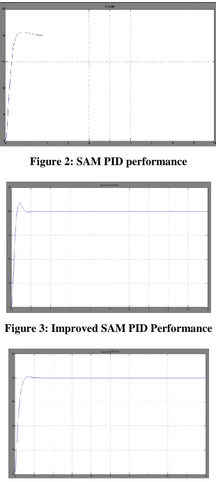
These three tuning methods are termed as Method 1, Method 2 and Method 3 in this literature. Auto-tune is carried out using these methods whose performance is shown in figure 2, figure 3 and figure 4. The various parameters are tabulated in Table 1.

(5)

International Journal of Emerging Technology and Advanced Engineering

59

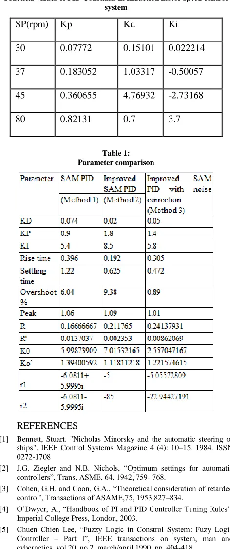
Method 1 algorithm is calculating this value by equating other PID parameters momentarily to zero hence there is no interdependent effects but method 3 algorithms dealing with interdependency of all PID parameters.

Proportional term is directly related to the speed of control action slow or fast. Moderate value of KP is suggested for better stability. Greater the value of KP thus faster is the controller. Method 2 has Kp=1.8 and rise time =0.192 whereas method 1 has Kp=0.9 and rise time=0.396. Thus the algorithm used for method 2 is acting faster than earlier SAM PID algorithm. Method 2 algorithm has shown the greater overshoot which is undesirable but method 3 has the much more improved value of 0.89 % (earlier 9.38 %).

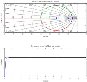
Figure 5, 6 and 7 shows the root locus of the three methods respectively. Performance of the system will be smooth and damping nature of output can be overcome by selecting real roots only. This is demonstrated with the help of Table 1 that only method 1 has complex roots whereas the other two methods have real roots only appearing on the right side of root locus.

System-II Control of Induction Motor

The system was developed in the laboratory. The block diagram of the experimental setup is shown in Fig. 8. The testing of the system is carried out under no load condition. The performance of the auto-tuned PID in controlling the Induction motor is just studied by varying the speed of the motor.

To prove the performance of Auto-tuned PID, the proposed controller is applied in the present Induction Motor for the speed control and its performance is recorded by taking the practical results at different set points. The practical result in Fig.9 and Fig.10 shows the successful implementation of auto-tuned PID controllers in the present Three Phase Induction Motor Control. The red horizontal line at Y-axis represents the set point of speed and the black curve represents the change in speed with time in seconds. The settling time of 0.6 sec. is obtained at both the set points. It is clear from the result of that the motor coverage to the desired speed with minimum overshoots. The ripple is almost disappearing in case of the proposed controller. The settling time gets improved with almost constant first peak time is achieved with the proposed SAM-PID controller by using the V/F control method. However, the peak overshoot is 40%.

VII. CONCLUSION

Presently improved tuning algorithm is acting faster and responds quickly to error signal then its earlier algorithm.

[image:5.612.366.521.324.669.2]

Noise corrected improved algorithm settle down in very short duration of time and overshoot approximately equal to less than 1% (Except 3-phase Induction Motor). In the noisy environment improved algorithm with a noise, the correction method is suggested. Thus, the new tuning algorithm tuned PID controller for faster response and better noise rejection property so that this algorithm is robust in the noisy environment. The roots of r1 and r2 should be real only and left the side of root locus for better stability and performance of the algorithm. The three-phase induction motor control by using SAM-PID controller is more stable and efficient. The auto tune algorithm is robust and demonstrates the performance in noisy environment. Thus, it can be used in various ways. To improve the system performance SAM-PID controller also has the feature of adaptive and optimal controlling.

Figure 2: SAM PID performance

Figure 3: Improved SAM PID Performance

(6)

International Journal of Emerging Technology and Advanced Engineering

[image:6.612.89.245.151.490.2]

60

[image:6.612.344.556.424.590.2]

Figure 5: root locus of SAM PID

Figure 6: root locus of improved SAM PID

Figure 7:- root locus of improved SAM PID with noise correction method.

Figure 8:- 3-phase induction motor control

Fig. 9 Plot of speed versus time (sec) at set point 800

0.0 0.2 0.4 0.6 0.8 1.0

0 100 200 300 400 500 600 700 S p ee d (r p m ) Time (S) Speed(rpm) Set Speed (rpm)

Fig. 10 Plot of speed versus time (sec) at set point 450

-25 -20 -15 -10 -5 0 5

-10 -5 0 5 10 0.87 0.93 0.97 0.992 0.24 0.46 0.64 0.78 0.87 0.93 0.97 0.992 5 10 15 20 25 0.24 0.46 0.64 0.78

Root Locus : SAM PID

Real Axis Im a g in a r y A x is

0 2 4 6 8 10 12 14 16 18 20

0 0.5 1 1.5

Step Response : SAM PID

Time (sec) A m p li tu d e

-300 -250 -200 -150 -100 -50 0 50 -100 -50 0 50 100 0.3 0.52 0.7 0.82 0.9 0.95 0.978 0.994 0.3 0.52 0.7 0.82 0.9 0.95 0.978 0.994 50 100 150 200 250 300

Root Locus : Improved SAM PID

Real Axis Im a g in a r y A x is

0 2 4 6 8 10 12 14 16 18 20

0 0.5 1 1.5

Step Response : Improved SAM PID

Time (sec) A m p litu d e

Root Locus : Improved SAM PID w ith noise correction

Real Axis Im a g in a ry A x is

0 2 4 6 8 10 12 14 16 18 20

0 0.5 1 1.5

Step Response : Improved SAM PID w ith noise correction

Time (sec) A m p litu d e

[image:6.612.94.244.518.658.2]

(7)

International Journal of Emerging Technology and Advanced Engineering

61

Table 2

Practical values of PID Constants in Induction motor speed control system

SP(rpm) Kp Kd Ki

30 0.07772 0.15101 0.022214

37 0.183052 1.03317 -0.50057

45 0.360655 4.76932 -2.73168

[image:7.612.49.285.151.713.2]

80 0.82131 0.7 3.7

Table 1: Parameter comparison

REFERENCES

[1] Bennett, Stuart. "Nicholas Minorsky and the automatic steering of

ships". IEEE Control Systems Magazine 4 (4): 10–15. 1984. ISSN 0272-1708

[2] J.G. Ziegler and N.B. Nichols, ―Optimum settings for automatic

controllers‖, Trans. ASME, 64, 1942, 759- 768.

[3] Cohen, G.H. and Coon, G.A., ―Theoretical consideration of retarded

control‘, Transactions of ASAME,75, 1953,827–834.

[4] O‘Dwyer, A., ―Handbook of PI and PID Controller Tuning Rules‖,

Imperial College Press, London, 2003.

[5] Chuen Chien Lee, ―Fuzzy Logic in Constrol System: Fuzy Logic

Controller – Part I‖, IEEE transactions on system, man and cybernetics, vol 20, no 2, march/april 1990, pp. 404-418

[6] Jong-Hwan Kim, Member, IEEE, Kwang-Choon Kim, and Edwin K.

P. Chong, Member, IEEE, ―Fuzzy Precompensated PID Controllers‖, IEEE transactions on control systems technology, vol. 2 , no. 4, december 1994 pp. 406-411

[7] Wei Li, Member, IEEE, ―Design of a Hybrid Fuzzy Logic

Proportional Plus Conventional Integral-Derivative Controller‖, IEEE transactions on fuzzy systems, vol. 6, no. 4, november 1998, pp. 449-463

[8] Kyoung Kwan Ahn and Bao Kha Nguyen, ―Position Control of

Shape Memory Alloy Actuators Using Self Tuning Fuzzy PID Controller‖, International Journal of Control, Automation, and Systems, vol. 4, no. 6, pp. 756-762, December 2006

[9] K. S. Tang, Member, IEEE, Kim Fung Man, Senior Member, IEEE,

Guanrong Chen, Fellow, IEEE, and Sam Kwong, Member, IEEE, ―An Optimal Fuzzy PID Controller‖, IEEE transactions on industrial electronics, VOL. 48, NO. 4, AUGUST 2001, pp. 757-765

[10] Zhen-Yu-Zhao, Member, IEEE, Masayoshi Tomizuka, IEEE and

Satoru Isaka, Member IEEE, ―Fuzzy Gain Scheduling of PID controller‖, IEEE transactions on system, man and cybernetics, vol 23, no 5, September/octomber 1993 pp- 1392-1398

[11] W. Li, X. G. Chang, Jay Farrell, and F. M. Wahl, ―Design of an

Enhanced Hybrid Fuzzy P ID Controller for a Mechanical Manipulator‖, IEEE transactions on systems, man, and cybernetics— part b: cybernetics, VOL. 31, NO. 6, DECEMBER 2001 pp- 938-945

[12] Un-Chul Moon, Member, IEEE, and Kwang Y. Lee, Fellow, IEEE,

―Hybrid Algorithm With Fuzzy System and Conventional PI Control for the Temperature Control of TV Glass Furnace‖, IEEE transactions on control systems technology, VOL. 11, NO. 4, JULY 2003, pp 548-554

[13] Isin Erenoglu Ibrahim Eksin Engin Yesil Mujde Guzelkaya, ―An

Intelligent Hybrid Fuzzy Pid Controller‖, Proceedings 20th European Conference on Modelling and Simulation ECMS, 2006 ISBN 0-9553018-0-7 / ISBN 0-9553018-1-5

[14] Jones, A.H.; De Moura Oliveira, P.B.; , "Genetic auto-tuning of PID

controllers," First International Conference on Genetic Algorithms in Engineering Systems: Innovations and Applications, 1995. GALESIA. (Conf. Publ. No. 414) , vol., no., pp.141-145, 12-14 Sep 1995 doi: 10.1049/cp:19951039

[15] Wang, P.; Kwok, D.P.; , "Auto-tuning of classical PID controllers

using an advanced genetic algorithm," Proceedings of the 1992 International Conference on Industrial Electronics, Control, Instrumentation, and Automation, 1992. Power Electronics and Motion Control., , vol., no., pp.1224-1229 vol.3, 9-13 Nov 1992 doi: 10.1109/IECON.1992.254429

[16] Liu Fan; Er Meng Joo; , "Design for auto-tuning PID controller

based on genetic algorithms," 4th IEEE Conference on Industrial Electronics and Applications, 2009. ICIEA 2009., vol., no., pp.1924-1928, 25-27 May 2009 doi: 10.1109/ICIEA.2009.5138538

[17] Zwe-Lee Gaing, Member, IEEE, ―A Particle Swarm Optimization

Approach for Optimum Design of PID Controller in AVR System‖, IEEE transactions on energy conversion, VOL. 19, NO. 2, JUNE 2004, pp. 384-391

[18] Shirazi, Mariko, Regan Zane, and Dragan Maksimovic. "An auto

tuning digital controller for DC–DC power converters based on online frequency-response measurement." IEEE Transactions on Power Electronics, 24.11 (2009): 2578-2588.

[19] Majhi, S., and D. P. Atherton. "Online tuning of controllers for an

(8)

International Journal of Emerging Technology and Advanced Engineering

62

[20] Jones, A. H., N. Ajlouni, and M. Uzam. "Online frequency domain

identification and genetic tuning of PID controllers." IEEE Conference on Emerging Technologies and Factory Automation, 1996. EFTA'96. Proceedings., 1996. Vol. 1. IEEE, 1996.

[21] Lago, Pedro, Teresa Mendonça, and Lio Goncalves. "Online

auto-calibration of a PID controller of neuromuscular blockade." IEEE

International Conference on Control Applications, 1998.

Proceedings of the 1998. Vol. 1. IEEE, 1998.

[22] Kookos, I. K., A. I. Lygeros, and K. G. Arvanitis. "On-line PI

controller tuning for integrator/dead time processes." European journal of control 5.1 (1999): 19-31.

[23] Schroder, P., et al. "Online genetic auto-tuning of mixed H2/H∞

optimal magnetic bearing controllers." International Conference on Control'98. UKACC (Conf. Publ. No. 455). IET, 1998.

[24] Huang, H-P., M-L. Roan, and J-C. Jeng. "On-line adaptive tuning for

PID controllers." IEE Proceedings-Control Theory and Applications 149.1 (2002): 60-67.

[25] Blažič, Sašo, et al. "Online fuzzy identification for an intelligent

controller based on a simple platform." Engineering Applications of Artificial Intelligence22.4 (2009): 628-638

[26] Gade S S, Shendge S B, Uplane M D,―On line Auto Tuning of PID

controller Using Successive Approximation Method,‖ IEEE International conference on Recent Trends in Information, Telecommunication and Computing (ITC-2010 cochin )12th – 13th March , Page numbers 277 - 280.

[27] Gade S S, Shendge S B, Uplane M D, ―Performance comparison of