discharge emanating from the
Gangotri glacier
by
Kirk Gunnar Larsen
A thesis submitted for the degree of
master of science
School of Environment and Life Sciences
College of Science and Technology
University of Salford, UK
List of Figures . . . iii
List of Tables . . . ix
Dedication . . . x
Acknowledgements . . . xi
Declaration . . . xii
Abstract . . . .xiii
1 Introduction . . . 1
1.1 Theses outline . . . 5
1.2 Aim & objectives . . . 6
2 Study Area . . . 8
3 Background . . . 16
3.1 The 0◦C isotherm and summer snowfall . . . 16
3.2 Retreat of the Gangotri glacier and other Himalayan glaciers . . 24
3.3 Himalayan streamflow . . . 31
4 Methods . . . 38
4.1 Discharge data . . . 38
4.2 Air temperature and precipitation data . . . 40
4.3 Data analysis . . . 40
5.1 Air temperature, precipitation and
discharge for the summers of 2001-2004 . . . 43
5.2 Interaction between discharge and precipitation in relation to the elevation of the 0 ◦C isotherm . . . 55
5.3 Interaction between discharge and air temperature in relation to the elevation of the 0 ◦C isotherm . . . 63
5.4 Specific summer snowfall events and the response of discharge . 71 6 Discussion . . . 77
6.1 Year to year trends in discharge, air temperature and precipitation 77 6.2 General influence of air temperature and precipitation on dis-charge . . . 82
6.3 Interaction of air temperature and precipitation with discharge, in relation to the elevation of the 0 ◦C isotherm . . . 86
6.4 Relationship between discharge, air temperature and precipita-tion during specific summer snowfall events . . . 90
7 Conclusion . . . 98
7.1 Summary of key findings . . . 98
7.1.1 Meeting the aim and objectives . . . 100
7.2 Limitations . . . 102
7.3 Considerations for future research . . . 102
1.1 Effects of a warming climate on discharge from a glacier (Hock
et al., 2005). . . 2
1.2 Four major climatic zones present within the Himalayas (Khan
et al., 2017). . . 4
1.3 Schematic diagram of monsoon rainfall over Gangotri glacier and Bhagirathi basin at differing elevations (Khan et al., 2017). 4
2.1 Span of the Himalayas across Pakistan, India, Nepal, Bhutan
and China. . . 9
2.2 The North West Garhwal Himalaya displaying glaciers and rivers
within Bhagirathi basin (Adapted from Sharma and Owen, (1996)). 10
2.3 Elevation zones as a percentage of the Bhagirathi basin and an
area-elevation curve (Singh et al., 2008). . . 11
2.4 Damage sustained by a major rockslide affecting Gangotri town.
(Haritashyaet al., 2006). . . 12 2.5 Cross sectional profile of Gangotri valley at varying distances
from the glacial snout (A. 2 km, B. 15 km, C. 23 km, D. 25 km),
with glacially eroded terraces marked by arrows (Baliet al., 2003). 14
2.6 Plan view of Gangotri valley including locations of each cross
section illustrated in Figure 2.5 (Baliet al., 2003). . . 15
3.1 How vertical movements of the 0◦C isotherm partitions differing
areas of a basin into parts which precipitation falls as rain or
snow, and how movement of the transient snow line influences
the snow covered and snow free areas of a basin (Collins, 1998b). 17 3.2 Linear regression displaying the relationship between 0◦C isotherm
3.3 Linear relationship between freezing level heights and mass
bal-ance for a number of glaciers located in High Asia (Wanget al.,
2014).(Continued. . .) . . . 20 3.3 Linear relationship between freezing level heights and mass
bal-ance for a number of glaciers located in High Asia (Wanget al.,
2014).(Concluded.) . . . 21 3.4 Changes in equilibrium line altitude (ELA) and freezing level
height (FLH) between 1958 and 2003 for ¨Ur¨umqi glacier (Zhang
and Guo, 2011). . . 22
3.5 Distance to the surface (d) and surface albedo for the
Morter-atschgletscher between Julian days 180 (June 28) and 210 (July
28) for the year 2000 (Oerlemans and Klok, 2004). . . 23 3.6 Glacier boundaries of the Gangotri glacier for 1962 and 2006
(Negi et al., 2012). . . 26
3.7 Cumulative length changes of selected glaciers located within
the Indian Himalaya (Bhambri and Bolch, 2009). . . 27
3.8 Images gathered via remote sensing of Tara Bamak glacier
dur-ing 1968 (a) and 2006 (b) (Bhambri et al., 2011). . . 28
3.9 Images gathered via remote sensing of the frontal area of
Gan-gotri glacier during 1968 (a) and 2006 (b) (Bhambri et al., 2011). 28
3.10 Cumulative length changes of glaciers located in the east, central and west Himalaya with the Karakoram region (Bolchet al., 2012). 30
3.11 Cumulative rainfall and discharge flowing from the Dokriani
glacier throughout the ablation season for the years 1994, 1998,
1999 and 2000 (Thayyen et al., 2005). . . 32
3.12 Daily total discharge (columns) and measured daily total
sus-pended sediment (line) from the Batura glacier between April
& October 1990 (Collins and Hasnain, 1995). . . 33
3.13 Diurnal discharge measured at Bhojbasa for Gangotri glacier,
3.14 Monthly summer variations of discharge at (A) Tela and (B)
Gujjar Hut and percentage contribution from the glacier
catch-ment (Thayyen and Gergan, 2010). . . 35 3.15 Mean monthly streamflow for Chenab River at Salal at current
air temperature and +2◦C (Arora et al., 2008). . . 36
3.16 Daily discharge from July to August from Dunagiri glacier for
1985 (a), 1987 (b), 1988(c) and 1989 (d) (Srivastava et al., 2014). 37
4.1 Stage-discharge relationship established for the ablation season
of 2000, 3 km downstream of the Gangotri glacier (Singh et al.,
2006b). . . 39
5.1 Daily average air temperature (◦C) at an elevation of 3800 m and daily total precipitation (mm) measured nearby to the snout of
Gangotri glacier, with daily average discharge measured 3 km
downstream for 2001 between Julian days 121 (May 1) and 293
(October 20). . . 45
5.2 Daily median air temperature (◦C) at an elevation of 3800 m
and daily total precipitation (mm) measured nearby to Gangotri
glacier, with daily average discharge measured 3 km downstream
for 2002 between Julian days 128 (May 8) and 293 (October 20). 47
5.3 Daily median air temperature (◦C) at an elevation of 3800 m and daily total precipitation (mm) measured nearby to Gangotri
glacier, with daily average discharge measured 3 km downstream
for 2003 between Julian days 129 (May 9) and 293 (October 20). 49
5.4 Daily median air temperature (◦C) at an elevation of 3800 m
and daily total precipitation (mm) measured nearby to Gangotri
glacier, with daily average discharge measured 3 km downstream
for 2004 between Julian days 128 (May 7) and 286 (October 12). 51
5.5 Discharge and precipitation for 2001 (A), 2002 (B), 2003 (C)
and 2004(D), with their R2 values and equations. . . 56 5.6 Discharge and precipitation for 2001 (A), 2002 (B), 2003 (C)
and 2004(D) filtered for when the 0◦C isotherm was positioned
5.7 Discharge and precipitation for 2001 (A), 2002 (B), 2003 (C)
and 2004(D) filtered for when the 0◦C isotherm was positioned
below 5000 m, with their R2 values and equations. . . 60 5.8 Discharge and precipitation for 2002 (A) and 2004 (B) filtered
for when the 0◦C isotherm was positioned below 4500 m, with
their R2 values and equations. . . 61
5.9 Discharge and air temperature for 2001 (A), 2002 (B), 2003 (C)
and 2004(D), with their R2 values and equations. . . 64
5.10 Discharge and air temperature for 2001 (A), 2002 (B), 2003 (C)
and 2004(D) filtered for when the 0 ◦C isotherm is positioned
below 5500 m, with their R2 values and equations. . . 66 5.11 Discharge and air temperature for 2001 (A), 2002 (B), 2003 (C)
and 2004(D) filtered for when the 0 ◦C isotherm is positioned
below 5000 m, with their R2 values and equations. . . 68
5.12 Discharge and air temperature for 2001 (A), 2002 (B), 2003 (C)
and 2004(D) filtered for when the 0◦C isotherm was positioned
below 4500 m, with their R2 values and equations. . . 69
5.13 Example of a summer snowfall event occurring in 2001,
includ-ing precipitation (columns), air temperature (dotted line) and
discharge (solid line). . . 72
5.14 Example of a summer snowfall event occurring in 2002, includ-ing precipitation (columns), air temperature (dotted line) and
discharge (solid line). . . 74
5.15 Example of a summer snowfall event occurring in 2004,
includ-ing precipitation (columns), air temperature (dotted line) and
discharge (solid line). . . 76
6.1 Daily total discharge (solid line) from Dokriani glacier and daily
total rainfall (bars) including mean daily temperature and
dis-charge without inclusion of the rainfall component (dotted line)
6.2 Modelled and measured daily discharge averaged over 2001 to
2006 for the Dischma catchment, Switzerland. (Bavay et al.,
2009) . . . 79 6.3 Precipitation within the Gangotri valley for 1999 (a) and 2000
(b) (Kumaret al., 2002) . . . 81
6.4 Example of a summer snowfall event occurring in 2001
high-lighted within the red area, including precipitation (columns),
air temperature (dotted line) and discharge (solid line). . . 91
6.5 Example of a summer snowfall event occurring in 2002
high-lighted within the red area, including precipitation (columns),
air temperature (dotted line) and discharge (solid line). . . 92
6.6 Example of a summer snowfall event occurring in 2004 high-lighted within the red area, including precipitation (columns),
air temperature (dotted line) and discharge (solid line). . . 92
6.7 Images of the Vernagtbach basin on the August 28, 2003 and
September 4 (2003), before and after a summer snowfall event
(Escher-Vetter and Siebers, 2007). . . 95
6.8 Discharge emanating from the Vernagtbach basin between
3.1 Total recession and rate of retreat for Gangotri glacier between
1935 and 2004 (Kumaret al., 2007). . . 25
5.1 Total precipitation for the summers of 2001 to 2004. . . 53
5.2 Average discharge, precipitation event and air temperature for
summers 2001 to 2004. . . 53
5.3 Summary of R2 between daily average discharge and daily total
precipitation for each year, under each filter with their
corre-sponding p-value. . . 62
5.4 Summary of R2 between daily average discharge and daily av-erage air temperature for each year, under each filter with their
corresponding p-value. . . 70
6.1 Correlation between daily average discharge and daily average
air temperature for each summer investigated. . . 82
6.2 Correlation between daily average discharge and daily total
pre-cipitation for each summer investigated. . . 83
6.3 Correlations between climatic variables measured at Zermatt
(Z), Sion (S) and Saas Almagell (SA) and total annual runoff (Collins, 1987). . . 84
6.4 Summary of correlations between daily average discharge and
daily total precipitation under differing 0 ◦C isotherm filters. . . 86
6.5 The glacierised area for different elevation ranges within the
Gangotri glacier basin (Singhet al., 2008). . . 88
6.6 Summary of correlations between daily average discharge and
6.7 Correlation between daily total precipitation and daily average
discharge before, during and after a specific precipitation event
eternally thankful . . .
I would first like to thank the late Professor David N. Collins, who first ignited
my love for Alpine glaciers leading me to undertake postgraduate study in the area. I will never forget David’s expertise, kind heartedness and
approacha-bility, not to mention the incredible field trips. For these opportunities and
experiences I am immensely grateful, making my time at the University of
Salford as great as it was.
My gratitude is also extended to both Dr Neil Entwistle and Dr Robert
Williamson for their help and support given throughout the duration of my
postgraduate study, in particularly during the difficult past year. Their
ap-proachable and helpful manner has been outstanding and without their
guid-ance the completion of this thesis would not have been possible. For this I am truly indebted.
I also wish to thank both of my parents Gary and Alison Larsen as well as
Linda Owens for the unrivalled support and encouragement they have supplied
during my study. This has been utterly invaluable to me and for this I am also
sincerely thankful.
Furthermore, I would also like to thank my friends who often provided
nec-essary distraction from time to time. Thanks also go to my fellow student
George Pea, who has been great company throughout both my undergraduate and postgraduate study, often providing much needed camaraderie.
I would also like to thank NERC for the funding of this project, without which
This is to certify that the copy of my thesis, which is presented for the degree
of Master of Science by research, embodies the results of my own course of research, has been completed by myself and has been viewed by my supervisor
before presentation.
Study of Himalayan glaciers are important for a number of reasons
includ-ing hydroelectric power, drinkinclud-ing water supply, irrigation & water resources.
The aim of this investigation was to determine how summer snowfall events
between 2001 & 2004 influenced runoff flowing from Gangotri glacier, located
in the Garhwal region of the Himalayas. This was achieved by collating air
temperature, precipitation and discharge data for the study area. Data were
used to determine the hydrological regime within catchment and to establish the general influence that air temperature and precipitation have on discharge,
using regression and correlation analysis. Using a temperature lapse rate the
daily average elevation for the 0 ◦C isotherm was calculated. This
differenti-ated days in which snowfall events would cover a large majority of the glacier
through filtering elevation. Correlation analysis was used to assess the
rela-tionship between air temperature and discharge; before, during and after these
precipitation events. It was found that air temperature was the driving factor
for discharge with R2 results ranging from 0.38 to 0.67 for the study period, whereas between discharge and precipitation R2 ranged from 0 to 0.16. Under lowering 0 ◦C isotherm filters the relationship between air temperature and
discharge became weaker for all years apart from 2004, whereas the
relation-ship between discharge and precipitation became more negative for 2001 &
2004. These findings suggest a decreasing influence of air temperature and
presence of snowfall, where an increase in precipitation causes a decrease in
discharge. During three specific snowfall events correlation between discharge
and air temperature before the snowfall event was positive, during the period
of snow cover was negative and after the snowpack had depleted returned to a
Introduction
Glaciers and ice caps occupy around 10% of the Earth’s land mass concentrated
primarily in polar regions, but are important in that they hold nearly 77% of
total fresh water. Himalayan glaciers alone store around 12 000 km3 of fresh
water and source some of the worlds largest rivers such as the Indus, Ganga
and Brahmaputra (Dyurgerov and Meier, 2005; Ninh, 2007). The Himalayas
are both the highest and youngest mountain range in the world, boasting the
largest glacial coverage outside of the polar regions and are sometimes referred to as ‘the third pole’ (Dyurgerov, 2001; Khanet al., 2017; Pandey et al., 1999;
Singh et al., 2014).
The Indian region of the Himalayas contains around 9 575 glaciers spanning
an area of nearly 40 000 km2 (Raina and Srivastava, 2014; Sangewar et al.,
2009). Himalayan glaciers and their study is of increasing importance to India
for a number of reasons including hydroelectric power, drinking water supply,
irrigation and other water resources. The demand for these resources is also
increasing due to pressures from industrial development and urbanisation as a result of rapid population growth (Singh et al., 2011).
Understanding glacial response to meteorological conditions including summer
snowfall events is also of increasing importance, due to a warming climate. A
century due to climate change, evident in a number of studies including those
conducted by Bahugunaet al., (2007), Kulkarni and Bahuguna, (2002),
Kulka-rni et al., (2007), and Yao et al., (2007). It has also been suggested by the Intergovernmental Panel on Climate Change that total glacier mass within
Alpine regions could decline by up to a quarter by 2050 and around half by
2100 (Watsonet al., 1996). The decline of glaciers within the Himalayan region
would be detrimental to near 500 million inhabitants who rely on meltwater
derived from glaciers within major rivers (Rees and Collins, 2006).
The potential effects of a warming climate on glaciers are displayed in
Fig-ure 1.1 from a study conducted by Hock et al., (2005), who investigated the
response of glacial discharge to climatic warming.
Figure 1.1: Effects of a warming climate on discharge from a glacier (Hock et al., 2005).
The diagram illustrated in Figure 1.1 displays the effect mass loss through
climatic warming has on glaciers including larger peak flows, more specific
runoff, reduction of firn volume and faster depletion of winter snow cover. The
depletion of winter snow cover is one of the most influential effects, as this
leaves more bare ice exposed to radiation leading to more glacier mass loss and
the further effects this causes (Hock et al., 2005). During a warming climate
flow cannot be sustained and will eventually begin to decrease and disappear
as the glacier declines in mass (Rees and Collins, 2006).
Within the Himalayas, monsoonal rainfall during summer plays a large role on the status of glaciers. The monsoon is predominantly caused by high
upper-tropospheric air temperatures above the Tibetan Plateau, through warming of
the land mostly situated at elevations above 3500 m. This produces a
temper-ature gradient between the Indian Ocean and Tibetan Plateau, causing warm
and moist air to rise upwards over the Himalayas which cools and produces
clouds forming the monsoon (Fu and Fletcher, 1985; Immerzeel et al., 2009;
Zhisheng et al., 2011).
The Indian summer monsoon weakens from east to west meaning the Hi-malayas can be split into 4 zones (Figure 1.2). Zone 1, furthest west, represents
a region mainly controlled by westerlies as opposed to monsoonal influences.
Glaciers located within the region of Zone 1 are influenced mainly by winter
precipitation. Zone 2, located over the Karakoram and western region of the
Himalayas, experiences both influence from monsoonal rainfall and a small
influence from the westerlies. Zone 3 is located in the Central Himalayan
re-gion and is predemonantly influenced by monsoonal rainfall including parts
of Tibet, Nepal and India, with many glaciers within this zone debris
cov-ered. Moreover, Zone 4 is located over the eastern most area where many of the glaciers are summer accumulation type due to domination of the summer
monsoon (Khanet al., 2017).
Distribution of monsoonal rainfall within the Bhagirathi basin containing
Gan-gotri glacier is evident in Figure 1.3. It is apparent that more rainfall occurs at
lower elevations of the basin, but some still occurs at higher elevations over the
glacier. If air temperature is low, causing a low elevation of the 0 ◦C isotherm
Figure 1.2: Four major climatic zones present within the Himalayas (Khanet al., 2017).
Literature directly investigating the effect of summer snowfall events on
dis-charge from glacierised basins appears to be rare, especially within the
Hi-malayan region. This may partly be due to difficulties recording data regarding meteorological conditions within the Himalayas and discharge from glacierised
basins. Poor accessibility to high altitudes, harsh weather and precipitous
terrains may cause logistical problems for transportation of equipment (Singh
et al., 2005b). The area of study is of importance as summer precipitation
events have the potential to offset melt for short periods of time within
sum-mer months, which may slightly extend the life span of a glacier, especially
those which experience monsoonal rainfall.
Work displayed in following chapters attempts to understand the effect that
specific summer snowfall events have on discharge from a highly glacierised basin, located in the Indian Himalayas. It is hypothesised that a summer
pre-cipitation event which falls as snow will have a dampening effect on discharge,
despite an increasing air temperature. It is also thought that as the elevation of
the 0 ◦C isotherm decreases, the relationship between precipitation and runoff
will become negative and the relationship between air temperature and runoff
will become weaker.
1.1
Theses outline
This thesis comprises of seven chapters including introduction, study area,
background, methods, results, discussion and conclusion. The introduction
includes a small background to the general topic area, explains why this area
of research is important and hypothesises what this investigation expects to
find. Introduction also includes aim & objectives, which sets out what the
study aims to achieve and describes objectives in order to meet this aim.
Study area aims to provide information about the immediate region in which the investigation is based and the background aims to provide an insight into
the current understanding of each subsection through examining current
snow-fall, retreat of Gangotri glacier and other Himalayan glaciers and Himalayan
streamflow.
The methods chapter entails how the data were gathered regarding discharge, air temperature and precipitation with the data analysis utilised. Chapter
5 quantifies results of the investigation in detail, comprising of sections
re-garding general air temperature, precipitation and discharge for the summers
of 2001-2004, the interaction between discharge and precipitation, interaction
between discharge and air temperature in relation to the elevation of the 0
◦C isotherm and displays specific summer snowfall events with response of
discharge. Chapter 6 contains the discussion, explaining and accounting for
results within Chapter 5, with the utilisation of literature. The discussion will
attempt to explain year to year trends in discharge, air temperature and pre-cipitation, general influence of air temperature and precipitation on discharge,
interaction of air temperature and precipitation with discharge in relation to
the elevation of the 0 ◦C isotherm as well as relationship between discharge,
air temperature and precipitation during specific summer snowfall events.
The conclusion will provide an overall summary of main themes and findings
presented within this thesis, and describe how the aim and objectives were met.
Concluding remarks regarding limitations of the study and considerations for
future research in the topic area are also included.
1.2
Aim & objectives
The overall aim of the research is to investigate how summer snowfall events
influence discharge emanating from Gangotri glacier. This is to provide an
insight as to the effect a specific snowfall event over the ablation area of the
glacier has on runoff, utilising calculation of the 0 ◦C isotherm elevation. The
period under analysis occurred between May and October ranging from 2001 & 2004, using data regarding precipitation, discharge and air temperature.
1. Determine the discharge and meteorological regime for Gangotri glacier.
Gathering previously collected meteorological data will allow for determination
of the discharge and meteorological regime within the immediate area of the glacier.
2. Establish daily average elevation of the 0 ◦C isotherm for each summer
day.
Calculating the elevation of the 0◦C isotherm for each summer day will enable
the determination of precipitation type (rain or snow) over Gangotri glacier.
3. Identify precipitation events where snowfall covers a large amount of the
ablation zone.
Summer precipitation events which fall as snow over a majority of the glacial
area, identified through the third objective will allow for the fulfilment of the
overall aim of the study. This is by collaborating such precipitation events
with discharge and air temperature in order to observe their direct effect on
Study Area
The Himalayan arc spans a length of around 2 500 km with a width of 200 km
to 250 km, crossing through India, China (Tibet), Bhutan, Nepal and Pakistan
as displayed in Figure 2.1 (Le Fort, 1975). The Himalayas were formed around
40-50 million years ago, when the Indian subcontinent collided with Asia
fol-lowing the breakup of Pangea. Due to their low density and buoyancy neither
plate subducted, causing the crust between two continents to thicken through
compressional forces. This produced rapid uplift forming the Himalayas, which still continues today (Molnar, 1986).
The Himalayas are often referred to as ‘the water towers of Asia’, due to
large amounts of snow and ice which are present supplying water via rivers
to millions of people. Meltwater which emanates from snow and ice feeds a
number of large river systems including the Brahmaputra, Ganges, Yangtze,
Mekong and the Yellow Rivers. The river basins cover a vast expanse of around
9 million km2, of which 2.8 million km2 are within the Hindu Kush region of the Himalayas alone. There are an estimated 54 000 glaciers located within the region spanning an overall area of around 61 000 km2 (Bajracharya and
Figure 2.1: Span of the Himalayas across Pakistan, India, Nepal, Bhutan and China.
The primary area of study is the Bhagirathi basin located within the North
West Garhwal region, Uttarakhand. This area contains Gangotri glacier which
is the largest of glaciers located within Garhwal as displayed in Figure 2.2,
adapted from a map created by Sharma and Owen, (1996). Gangotri glacier
will be the primary glacier investigated, spanning an elevation of 4000 m to
The total area of different elevation zones for the Bhagirathi basin and their
individual percentage of total basin area are illustrated in Figure 2.3 created
by Singhet al., (2008). In 1999 Bhagirathi basin contained around 238 glaciers covering nearly 12% of the basins total area, with the Bhagirathi River flowing
from this valley being one of the main tributaries to the Ganga (Dobhal and
Mehta, 2010). Gangotri glacier itself is a product of a number of joining glaciers
including Swachand, Maiandi, Ghanohim and Kirti glaciers, with Chaturangi
glacier (Figure 2.2) also joining until 1971, before retreating 100 m (Vohra,
1988). Gangotr i Glacier Chaturangi Glacier Raktavarn Glacier Meru Glacier Manda Rudugaira Glacier Dudu Kedar Glacier Mecha Jaonil Glacier Dokriani Glacier Goni Chalan Glacier Bhatiakunt Glacier
Sian Glacier Rahtia Glacier Lamkhaga Glacier Kalapani Glacier River Bhagir athi
Figure 2.3: Elevation zones as a percentage of the Bhagirathi basin and an area-elevation curve (Singh et al., 2008).
In terms of geomorphology, the Bhagirathi basin is located within an active
and relatively young tectonic mountain range. Bhagirathi basin has steep sides
extending down to the Bhagirathi River, which flows east-northeast to
which Bhagirathi basin lies is still seismically active and continues to
experi-ence rapid uplift exposing augen gneiss, quartzites, phylites and granites. A
combination of fluvial incision, heavy monsoonal rainfall and earthquakes also mean that mass movements such as landslides are relatively common (Barnard
et al., 2004).
A recent example of a mass movement event that occurred in Bhagirathi basin
was investigated by Haritashyaet al., (2006) who studied hydro-meteorological
conditions of a storm that occurred in June 2000, causing unusually high levels
of precipitation on the upper region of the river. The storm induced a number
of rockslides/landslides between the snout of Gangotri glacier and Gangotri
[image:26.595.113.512.318.579.2]town causing damage such as that displayed in Figure 2.4.
Figure 2.4: Damage sustained by a major rockslide affecting Gangotri town. (Haritashyaet al., 2006).
In addition to causing damage to the town, a rockslide blocked the Bhagirathi
sudden high river flow downstream peaking at 124 m3s−1. This resulted in a rise of the river bed of around 3 m and a change in the rivers course (Haritashya
et al., 2006).
The valley containing Gangotri Glacier is a U-shaped valley, which is around
1.5 km wide where the glacial snout lies. Downstream of the glacial snout the
valley is marked by a number of debris cones, out-wash plains and recessional
moraines formed by previous glacial extent. The Bhagirathi River has incised a
V-shaped valley into the bottom of the U-shaped valley, as displayed in Figure
2.5 due to its high velocity caused by a steep gradient. The geographical
location within the Gangotri valley of each cross section are further illustrated
in Figure 2.6.
The fast flowing nature of the Bhagirathi River provides high sediment
trans-port capacity during peak flow, carrying sediments associated with glacial
erosion. Where the river experiences low gradients in wide areas of the valley
there is much deposition of glacial outwash, creating multiple channels of a
Figure 2.5: Cross sectional profile of Gangotri valley at varying distances from the glacial snout (A. 2 km, B. 15 km, C. 23 km, D. 25 km), with glacially eroded
Background
Gangotri glacier and wider Himalaya have been the subject of investigation
by many researchers for a number of years regarding glacial retreat and
dis-charge from glacierised basins, such as that containing Gangotri glacier. Such
research is of particular importance for planning and management of water
resources and also the design and operation of engineering projects including
hydropower (Singhet al., 2005a). Alford and Armstrong, (2010) state that as
a result of retreat; Ganga, Brahmaptra and other rivers located in North India could become more seasonal rivers in future, with decline of glaciers in the
Himalayas. This suggests that research of streamflow from glacier fed rivers
will become of increasing importance as glaciers decline, building upon those
already conducted.
3.1
The 0
◦C isotherm and summer snowfall
Elevation of the 0 ◦C isotherm is of great importance to glaciers around the
world, but is an area which has experienced little research focusing particularly
on high mountain glaciers, especially within the Himalayas. This is due to a
lack of high elevation weather stations which can only partly be substituted
isotherm or ‘freezing level’ as “The elevation above sea level at which the
air temperature is close to 0◦C”. Elevation of the 0 ◦C isotherm determines
whether precipitation falls as rain or snow, effectively splitting basins into two zones whereby precipitation which falls below the 0 ◦C isotherm falls as rain
and above falls as snow, evident in Figure 3.1 (Collins, 1998b).
Glaciers that encounter heavy monsoonal rainfall during summer are often
summer accumulation type and changes in air temperature at high altitude in
these regions may alter their accumulation pattern (Higuchi and Ohata, 1996).
Figure 3.1 displays how changes in elevation of the 0 ◦C isotherm determines
areas within a glacierised basin which receive rain or snow, and also displays
how movement of the transient snow line effects the percentage of snow covered
[image:31.595.134.504.345.554.2]and snow free areas.
Figure 3.1: How vertical movements of the 0◦C isotherm partitions differing areas of a basin into parts which precipitation falls as rain or snow, and how movement
of the transient snow line influences the snow covered and snow free areas of a basin (Collins, 1998b).
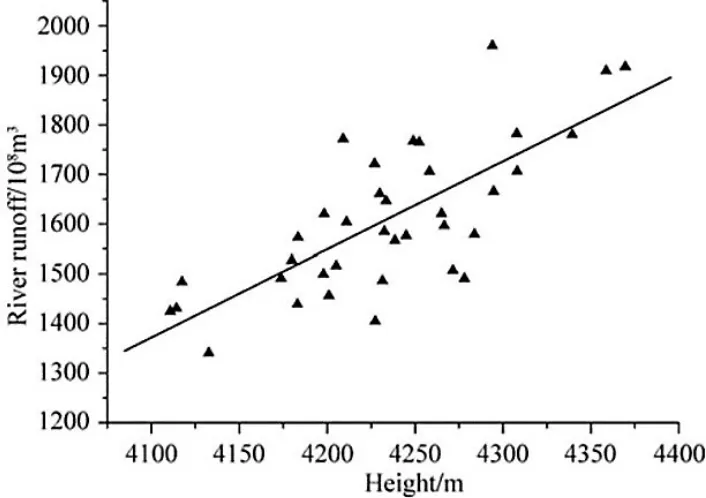
A study conducted by Zhang et al., (2010) investigated response of runoff to
movement of the summer 0◦C isotherm over the Xinjang region. It was found
and runoff, as displayed in Figure 3.2. This indicates that as elevation of the
0 ◦C isotherm increases, as do measurements of runoff and vice versa. This is
because as the height of the 0 ◦C isotherm increases, it is usually followed by a glaciers equilibrium line creating a larger ablation area and therefore more
runoff during summer. The regression coefficient between variables is also high
at 0.74, indicating that 74% of the runoff value can be explained by height of
[image:32.595.123.476.249.498.2]the 0 ◦C isotherm.
Figure 3.2: Linear regression displaying the relationship between 0 ◦C isotherm height and runoff from Xinjang (Zhanget al., 2010).
Wang et al., (2014) investigated freezing level heights in High Asia utilising
NCEP/NCAR reanalysis and its effects on glacier changes. Figure 3.3 displays
the findings of Wang et al., (2014) in terms of relationship between freezing
level height and mass balance for a large number of glaciers.
All glaciers investigated in Figure 3.3 encounter a negative relationship of differing severities between mass balance and freezing level heights. Glaciers
Shum-skiy (Figure 3.3d & 3.3e). Whereby as atmospheric freezing level height
in-creases, mass balance of each glacier steeply decreases. This indicates that
as air temperature potentially increases in the future, height of the freezing level will also increase and therefore decrease the mass balance of a number of
glaciers, causing shrinkage. This is evident in areas such as Eastern Tianshan,
Altai and Qilian Mountains which are all areas that have experienced largely
increasing trends of freezing level heights (Wang et al., 2014).
Moreover, a study conducted by Zhang and Guo, (2011), using atmospheric
air temperature gathered from the Chinese radiosonde network, found upward
trends for the freezing level height between 1958 and 2005 which appeared to
be consistent with retreat of the High Asian cryosphere. Figure 3.4 published
by Zhang and Guo, (2011) shows that equilibrium line altitude for ¨Ur¨umqi glacier follows patterns displayed by freezing level height, indicating a strong
Figure 3.4: Changes in equilibrium line altitude (ELA) and freezing level height (FLH) between 1958 and 2003 for ¨Ur¨umqi glacier (Zhang and Guo, 2011).
The primary source of heat for glacial melt is derived from incoming shortwave
solar radiation. Surface albedo of a glacier essentially determines how much shortwave solar radiation is absorbed and how much is reflected, measured on
a scale from 0 - 1. Ice surface albedo ranges from around 0.4 - 0.6, whereas the
surface albedo of fresh snow is around 0.9. This difference in surface albedo
has a large influence on the volume of runoff produced and also effects glacial
mass balance. On June 21 when solar radiation reaches its maximum, much
snow cover gathered from the previous winter will still be present resulting in
much of the incoming solar radiation being reflected. As the transient snowline
retreats exposing large areas of bare ice, the surface albedo of the glacier will
reduce causing an increase in melt rate and therefore runoff. Additionally, if altitude of the freezing level is low during a large summer precipitation event it
can cause snow to fall on exposed glacial ice as opposed to rain. The addition
of fresh snow may temporarily raise the albedo of the glacial surface and offset
This is demonstrated in a study conducted by Oerlemans and Klok, (2004),
who investigated the effect of summer snowfall on glacier mass balance for
Morteratschgletscher, Switzerland with their findings displayed in Figure 3.5.
Figure 3.5: Distance to the surface (d) and surface albedo for the
Morteratschgletscher between Julian days 180 (June 28) and 210 (July 28) for the year 2000 (Oerlemans and Klok, 2004).
Results displayed in Figure 3.5 demonstrate distance to surface of the glacier
measured using a sonic ranger and surface albedo (half hourly between
0800-1600), with measurements taken between Julian days 180 (June 28) and 210
(July 28) during 2000. The snowfall event occurs on Julian day 192 (July 10) shown by distance to surface of the glacier decreasing indicating build
up of a snowpack. Corresponding with build up of the snowpack, albedo of
ice in the study area increases from 0.3 to around 0.75. Low albedo of fresh
snow can be explained by melting beginning almost immediately slightly
low-ering its albedo, but still protects underlying glacial ice (Oerlemans and Klok,
2004). Oerlemans and Klok, (2004) concluded that heavy summer snowfall
reducing the amount of absorbed radiation and simultaneously adding mass.
A study regarding the role of snow-albedo feedback and warming of high
ele-vation Himalayas was conducted by Ghatak et al., (2014). Using Community Climate System Model version 4 and Geophysical fluid Dynamics Laboratory
model, Ghatak et al., (2014) found that surface albedo decreases more at
higher elevations than lower elevations due to retreat of the 0 ◦ isotherm and
snow line. Decrease in surface albedo and consequential increase in absorbed
solar radiation causes an increased loss of snowpack, triggering warming over
Central Asian mountains, Himalayas and Karakoram. A study conducted by
Fujita, (2008) investigated influence of precipitation seasonality on mass
bal-ance, also concluded that decreased summer snowfall on glaciers would cause
accelerated melting through a lowering of surface albedo.
3.2
Retreat of the Gangotri glacier and other
Himalayan glaciers
According to Jain, (2008) Gangotri glacier has only experienced 18 km of
retreat over a period of around 4000 years, when the snout of Gangotri glacier was positioned at Gangotri temple. Gangotri glacier advanced during the
little ice age between the 16th and 18th centuries, but has experienced rates
of recession between 22 m and 27 m per year over the past few decades. Jain,
(2008) also studied the effect that retreat of Gangotri glacier would have on
the Ganga. It was found that although Gangotri glacier had retreated around
22-27 m per year, there was no profound effect on flow of the Ganga and may
have little effect as it continues to retreat in the future, as beyond the nearby
Haridwar its sole influence on the Ganga dwindles to less than 4%.
Retreat of Gangotri glacier was also investigated by Kumaret al., (2007) using rapid static and kinematic GPS survey. Using the GPS in rapid static mode
revealed Gangotri glacier had experienced differing rates of retreat between
dis-played in Table 3.1. Table 3.1 also shows that rate of retreat declined to 17.15
ma-1 between 1971 to 2004 as opposed to 26.50 ma-1 recorded between 1935 and 1971.
Table 3.1: Total recession and rate of retreat for Gangotri glacier between 1935 and 2004 (Kumaret al., 2007).
Gangotri glacier was further investigated by Negiet al., (2012) who monitored
the glacier using remote sensing and ground observations. It was found that
prevailing wet snow conditions have caused slope scouring leading to soil and debris deposition onto the surface of Gangotri glacier. This debris cover is said
to be one of the main factors causing fast melting of the glacier and appears
to be impacting the glaciers health in an influential manner, finding overall
glacial area loss to be 6%. Figure 3.6 displays boundaries of the Gangotri
glacier for 1962 and 2006. It is evident that the glacier has experienced retreat,
Figure 3.6: Glacier boundaries of the Gangotri glacier for 1962 and 2006 (Negi
et al., 2012).
An investigation conducted by Bhambri and Bolch, (2009) mapping glaciers in
the Indian Himalayas produced a graph displaying cumulative length changes
of Indian Himalayan glaciers including Gangotri glacier as displayed in Figure
Figure 3.7: Cumulative length changes of selected glaciers located within the Indian Himalaya (Bhambri and Bolch, 2009).
Findings of Bhambri and Bolch, (2009) within Figure 3.7 indicate that
Gan-gotri glacier declined at a steady rate between years 1840 and 1960. After 1960
Gangotri glacier along with a number of other glaciers begin to experience a
rapid shortening of cumulative length, indicating rapid retreat for all glaciers
selected. With regards to Gangotri glacier in particular, cumulative length
change appears to drop from around −1000 m in 1960 to around −2250 m in 2009, much steeper than cumulative length change experienced between 1840
and 1960 of around −900 m over a longer period of time.
Bhambri et al., (2011) also investigated glacial retreat using remote sensing
in the Himalayas but focused on those located within the Garhwal Himalaya,
including Gangotri glacier. Figures 3.8 & 3.9 display area changes for Tara
Figure 3.8: Images gathered via remote sensing of Tara Bamak glacier during 1968 (a) and 2006 (b) (Bhambriet al., 2011).
Results obtained by Bhambri et al., (2011) (Figures 3.8 & 3.9) show large
changes in both glaciers between 1968 & 2006. The image of Tara Bamak
glacier in Figure 3.8a is a Corona image taken in 1968, the outline of which is laid over an ASTER image taken in 2006 (Figure 3.8b). It is evident that
much of retreat suffered by Tara Bamak glacier has not only been effecting the
snout, but has also experienced retreat in its north-eastern region by splitting
of an ice mass from the main body.
In terms of Gangotri glacier, the 1968 Corona image (Figure 3.9a) and 2006
Cartosat-1 image (Figure 3.9b) focus on the snout. It is clear from Figure 3.9
that the snout of Gangotri glacier has experienced much retreat between 1968
and 2006 with the amount of area lost around 0.38 km2. Bhambriet al., (2011) state that the number of glaciers located in Garhwal Himalaya increased from 82 to 88 between 1968 and 2006 due to fragmentation of large glaciers, with
recession rates between 1990 and 2006 increasing.
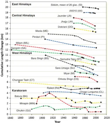
There has also been much research conducted on glacial retreat for many other
glaciers located in the Himalayas. Bolch et al., (2012) conducted research
regarding the cumulative length changes of a number of Himalayan glaciers,
Figure 3.10: Cumulative length changes of glaciers located in the east, central and west Himalaya with the Karakoram region (Bolch et al., 2012).
It is clear from Figure 3.10 that a large majority of glaciers located in the
Himalayas are experiencing retreat, especially after the 1970s. All appear to be
retreating apart from Batura, Minapin and Ghulkin located in the Karakoram
region, which all appear to be in advance or stable. It was also found that 25%
or stable between years 1976 and 2007.
Glacial retreat in the Himalayas was also investigated by Dobhal and Mehta,
(2010), who focused on Dokriani glacier using fixed date observations at the end of ablation period each year. It was found that Dokriani glacier has experienced
large changes in elevation and surface morphology. Between 1962 and 1991
total retreat of Dokriani glacier was measured at around 480 m meaning the
average rate of retreat for this period was 16.5 m/yr. Rate of retreat increased
to 17.8 m/yr between 1991 and 2000, but declined to 15.7 m/yr between 2000
and 2007 indicating that the rate of terminus retreat has recently declined
(Dobhal and Mehta, 2010).
3.3
Himalayan streamflow
The Indian monsoon also has a large influence on streamflow from glaciers
located in eastern and central Himalayas. The findings of Singh et al., (2000)
suggested a prominent role of monsoonal rainfall in determining runoff from
Dokriani glacier during July and August. Graphs illustrated in Figure 3.11
demonstrate cumulative discharge and rainfall for Dokriani glacier created by
Thayyen et al., (2005). The smooth curve of discharge measured throughout the ablation season of each year shows a similar trend to that of rainfall over
the same period of time. Although discharge and rainfall show a similar trend,
Thayyenet al., (2005) concluded that rise in discharge during the monsoon
pe-riod is more related to rising summer air temperatures as opposed to increased
Figure 3.11: Cumulative rainfall and discharge flowing from the Dokriani glacier throughout the ablation season for the years 1994, 1998, 1999 and 2000 (Thayyen
et al., 2005).
Seasonal variation of daily total discharge and measured daily total suspended
sediment for Batura glacier is illustrated within Figure 3.12, from April to
October. It is evident from Figure 3.12 that discharge begins to rise in early May, with the rise of the transient snowline during late June almost doubling
discharge before rapidly decreasing after early August. This is caused by
move-ment of the transient snowline which in turn causes the ablation zone of the
glacier to grow, creating a marked increase in discharge observed during the
summer period as the albedo of snow (0.9) is much higher than that of ice
Figure 3.12: Daily total discharge (columns) and measured daily total suspended sediment (line) from the Batura glacier between April & October 1990 (Collins and
Hasnain, 1995).
Moreover, Singh et al., (2005a) also investigated variations in discharge and
suspended sediment but on a diurnal scale from Gangotri glacier.
Measure-ments for discharge were gathered at a gauging site established at Bhojbasa,
around 3 km downstream of the terminus of Gangotri glacier. Figure 3.13
Figure 3.13: Diurnal discharge measured at Bhojbasa for Gangotri glacier, regarding clear days of the ablation period 2001 (Singh et al., 2005a).
Findings of Singh et al., (2005a) displayed in Figure 3.13 show a similar trend
to those displayed in Figure 3.12 by Collins and Hasnain, (1995). It is evident
in Figure 3.13 that discharge begins to rise in June and achieves its highest level during July, before beginning to decline. Results in Figure 3.13 also
indicate that during the first part of the melt season (May-June), discharge is
determined by extent of snow cover within the basin and snow depth (Singh
et al., 2005a).
Discharge was also investigated by Thayyen and Gergan, (2010) for Dokriani
glacier between 1998 and 2004 measured at Tela and Gujjar Hut. As with
pre-vious figures, Figure 3.14 shows that discharge flowing from Dokriani glacier
also peaks between July and August. It is also displayed in Figure 3.14 that
discharge from the glacier has begun to decrease over the years, despite
[image:49.595.121.504.156.482.2]per-centage contribution from the glacier catchment increasing.
Figure 3.14: Monthly summer variations of discharge at (A) Tela and (B) Gujjar Hut and percentage contribution from the glacier catchment (Thayyen and
Gergan, 2010).
An investigation conducted by Aroraet al., (2008) uses the SNOWMOD model
to research how potential increases in air temperature by +1◦C, +2◦C and
+3◦C affect streamflow from Chenab river basin, located in the western
Hi-malayas with an elevation ranging from 305 to 7500 m and a total glacierised area of 2.280 km2. The results in Figure 3.15 display total streamflow for
Chenab River measured at Salal between 1996 and 1999 with a simulated
Figure 3.15: Mean monthly streamflow for Chenab River at Salal at current air temperature and +2◦C (Arora et al., 2008).
The findings of Arora et al., (2008) displayed in Figure 3.15 show that with
an air temperature increase of +2◦C timing of when peak flow occurs for the
river remains the same around July and August. But their magnitude often
increases with an average increase of 19%, although this is not reflected within
winter streamflow.
Discharge originating from Dunagiri glacier in response to climate was the topic
of research for Srivastava et al., (2014). Dunagiri glacier lies at an altitude of 4200 m and is located within the Garhwal Himalaya of India. The study
focuses on years 1985, 1987, 1988 and 1989 over the ablation season from July
to September utilising daily values of discharge for each year, results of which
Figure 3.16: Daily discharge from July to August from Dunagiri glacier for 1985 (a), 1987 (b), 1988(c) and 1989 (d) (Srivastava et al., 2014).
Daily discharge displayed in Figure 3.16 shows that the largest peaks in
dis-charge for each year occur within July, with August displaying both increasing
and decreasing trends from year to year and September indicating a generally
decreasing trend for each year. Srivastava et al., (2014) also found that
abla-tion of Dungiri glacier was exponentially correlated with mean air temperature
Methods
Discharge data were obtained for Gangotri glacier between May & October
from 2001 to 2004. Precipitation and air temperature observations for the
same period, collected at Bhojbasa were also obtained. In the Indian
Hi-malaya, streamflow and meteorological monitoring sites located at high
alti-tudes nearby to glaciers are rare and most of which do not measure regularly,
indicating an inadequate hydrological and meteorological network in this area.
This makes acquisition of a long and complete data series on hydrometeorol-ogy for the Gangotri glacier and other glaciers difficult with few data sources
(Bolch et al., 2012; Chalise et al., 2003; Gurung et al., 2017; Singh et al.,
2006b).
4.1
Discharge data
Data gathered by Singh et al., (2006b) for discharge deriving from Gangotri glacier was measured around 3 km downstream of the snout. This area was
chosen as it met requirements of being a single channel with low turbulence and
was an accessible location. On the bank of the river a stilling well and concrete
wall were constructed with an automatic water level recorder placed on the
was also installed in order to calibrate the automatic recorder using manual
measurements. Discharge was estimated using a velocity-area technique, with
surface velocity of discharge measured utilising wooden floats and was found to be between 0.5 m s−1 and 4.5 m s−1, with mean velocity calculated by reducing
surface velocity by 10%. The area of cross section was measured using sounding
rods at the beginning and end of the melt season.
A stage-discharge relationship was then created for each year, in order to
convert measurements of water levels from the automatic water level recorder
into discharges utilising data collected from a range of flow stages. Figure 4.1
[image:53.595.123.496.312.627.2]displays the stage-discharge relationship created for 2000.
The method of estimating discharge for a river through the velocity-area
tech-nique has also been utilised by a number of other studies including those
conducted by Chhetri et al., (2016), Hood and Hayashi, (2015), Kumar et al., (2016), and Srivastava et al., (2014).
4.2
Air temperature and precipitation data
Air temperature and precipitation data for Gangotri glacier were collected
by Singh et al., (2005b), by establishing a meteorological observatory nearby
to the glacier terminus on the valley floor, situated at around 3800 m above sea level. The meteorological observatory used to collect relevant data was
equipped with a range of equipment including maximum and minimum
ther-mometers, anemometer, a self recording rain gauge, an ordinary rain gauge,
dry and wet bulb thermometers, evaporimeter, hydrograph, wind vane, a
sun-shine recorder and anemometer.
Timings for data collection taken by Singh et al., (2005b) were in concordance
with practice used by the India Meteorological Department providing daily
values for minimum and maximum air temperature and daily total values for
precipitation.
4.3
Data analysis
Data for discharge, air temperature and precipitation were collated in order to
perform data analysis investigating the 0◦C isotherm, summer snowfall events
and the effect these summer snowfall events had on discharge.
Daily average air temperature was first calculated from the maximum and minimum data and was then used to work out daily average elevation of the 0
◦C isotherm using a temperature lapse rate. The temperature lapse rate used
is derived from a study conducted by Singh et al., (2008), who investigated
a temperature lapse rate of 0.6◦C/100 m. A number of other studies also
found the temperature lapse rate of mountain regions to be between 0.5 and
0.7◦C/100 m including those conducted by de Scally, (1997), Hagemann et al., (2013), Luetschg et al., (2008), Singh and Jain, (2002; 2003), and Six and
Vincent, (2014).
Elevation of the 0 ◦C isotherm was calculated by using an equation based on
that utilised by both Singh and Jain, (2003) and Singhet al., (2008) in order to
calculate air temperature at specific elevations using only one meteorological
observatory, as given below:
Ti,j =Ti,base−δ(hj−hbase) (4.1)
where Singh and Jain, (2003) and Singhet al., (2008) describe components as
Ti,j being a measure of mean daily temperature on theith day, in the jth zone
measured in (◦C); Ti,base is daily mean temperature (◦C) on theith day at the
meteorological observatory, hj is hypsometric mean elevation (m) of the zone
investigated, hbase is elevation of the meteorological observatory (m) and δ is
the temperature lapse rate for the area (◦C/100 m).
Equation 4.1 was then modified in order to calculate daily average elevation of
the 0◦C isotherm within the basin containing Gangotri glacier as given below:
Eiso =
Ti,base
δ
!
+hbase (4.2)
where Eiso is elevation of the 0◦C isotherm; Ti,base is mean daily temperature
(◦C) on the ith day measured at the meteorological observatory, δ is the
tem-perature lapse rate for the area (0.6◦C/100 m) andhbase is the elevation of the
meteorological observatory.
Once established, Equation 4.2 was then applied to average air temperature
for each Julian day available using a temperature lapse rate of 0.6◦C/100 m,
for 2001 to 2004 collected by Singh et al., (2005b).
day, data were then filtered to only show air temperature, precipitation and
discharge on Julian days where the 0◦C isotherm was positioned below certain
elevations within the basin; including 5500 m, 5000 m and 4500 m. The starting elevation of 5500 m was chosen as this is around the mid point of Gangotri
glacier and subsequent filter elevations (5000 m & 4500 m) were chosen to give
an insight into how discharge was influenced by summer snowfall covering
almost the entire area of the glacier. Equation 4.1 was also used in order to
calculate average air temperature for each Julian day at the same elevations
used to filter data regarding the elevation of the 0 ◦C isotherm.
Once the data had been filtered for each elevation, correlation and regression
analysis were then performed on the data in order to determine the interaction
between summer snowfall events, discharge and elevation of the 0◦C isotherm. Filters were also used to identify individual summer snowfall events, which
were isolated and investigated in order to gather a more detailed account of
their specific effect on discharge. This was achieved using correlation analysis
on three specific periods around selected precipitation events. The first period
was before the snowfall event occurred, second was the snowfall event including
duration of which the snow cover endured and the third period was immediately
Results
The following section displays the results and analysis of this investigation
including air temperature, precipitation and discharge for the study period,
interaction between discharge and precipitation along with air temperature in
relation to altitude of the 0 ◦C isotherm and specific summer snowfall events
with the response of discharge.
5.1
Air temperature, precipitation and
discharge for the summers of 2001-2004
Discharge, air temperature and precipitation collected by Singhet al., (2006b)
and Singh et al., (2005b) for the summers of 2001 to 2004 are displayed in
Figures 5.1 to 5.4.
Over the summer of 2001 (Figure 5.1), daily average air temperature displays a generally arcing trend, although greatly fluctuates. The first value occurs on
Julian day 121 (May 1) with a temperature of 7.75◦C, which shows a generally
rising trend before reaching 14.25◦C on Julian day 188 (July 7) which is also
recorded on Julian day 202 (July 21). After the value of 14.25◦C on Julian
reaching its lowest value of 2.85◦C on Julian day 292 (October 19) after a sharp
drop from 8.35◦C on Julian day 283 (October 10). This occurs just before the
last value of 5.15◦C on Julian day 293 (October 20). Air temperatures of 14.25◦C recorded on Julian days 188 (July 7) and 202 (July 21), are 0.35◦C
(2.52%) higher than any other peak air temperature recorded within the time
period. The lowest value of 2.85◦C is 2.25◦C (44.12%) lower than any other
period of low air temperature recorded, before a drop in air temperature which
occurred on Julian day 283 (October 10). The average air temperature for 2001
was 9.84◦C.
Daily precipitation for 2001 is also illustrated. Although there appear to be
a number of summer precipitation events, none of that which occur are of a
considerably high magnitude, with average summer precipitation for the year only reaching 2.35 mm. The largest precipitation event recorded occurs on
Julian day 136 (May 16) with a value of 10.4 mm, 0.6 mm (6.12%) higher than
any other precipitation event recorded for that year. Total precipitation for
the summer of 2001 was 131.35 mm.
The trend within daily discharge in Figure 5.1 characterises a sharp increase,
peaking on Julian day 203 (July 22) with 176.70 m3s−1, rising from the lowest value of 8.50 m3s−1 on Julian day 121 (May 1). After two large drops in dis-charge between the largest peak occurring on Julian day 203 (July 22) and the second peak of 174.00 m3s−1 on Julian day 226 (August 14), discharge begins
to steadily decline before reaching 20.80 m3s−1on Julian day 293 (October 20).
Two peaks occurring on Julian days 203 (July 22) and 226 (August 14) were
32.50 m3s−1 (22.54%) and 29.80 m3s−1 (20.67%) higher respectively than any
other high flow event for discharge recorded. The lowest recorded discharge
for 2001 (8.50 m3s−1) occurs on Julian day 121 (May 1) attaining 12.30 m3s−1
Figure 5.1: Daily average air temperature (◦C) at an elevation of 3800 m and daily total precipitation (mm) measured nearby to the snout of Gangotri glacier, with daily average discharge measured 3 km downstream for 2001 between Julian days
Similarly to daily average air temperature for 2001, data for 2002 (Figure 5.2)
also shows a generally arcing trend, but appears to encounter more extreme
temperature variations. The series begins on Julian day 128 (May 8) at 8.45◦C and initially shows a generally rising trend, although displaying large variations
in air temperature. Examples of such variation include that recorded for Julian
day 141 (May 21), indicating an unusually low value of 4.55◦C and the highest
of the series for Julian day 175 (June 24) with 16.00◦C (1.65◦C warmer than
any other peak for 2002). After Julian day 198 (July 17) daily average air
temperature then begins to show a decreasing trend reaching its lowest point
on Julian day 250 (September 7) with an average temperature of 1.75◦C closely
followed by Julian day 256 (Septeber 13) with 2.10◦C, only 1.00◦C (36.36%)
and 0.65◦C (23.64%) lower than any other low temperature event recorded in the series. The series then ends on Julian day 293 (October 20) with 3.50◦C
and an average air temperature for the year of 9.25◦C.
Precipitation recorded for 2002 (Figure 5.2), displays almost entirely different
characteristics to that of 2001. Between Julian days 120 (April 30) & 215
(August 3) there only appears to be a small summer precipitation events,
highest of which occurring on Julian day 135 (May 15) producing 4.7 mm of
precipitation. Between Julian days 216 (August 4) & 257 (September 14)
there appears to be a large number of precipitation events, most are high
in magnitude. Precipitation appears to build up, starting on Julian day 216 (August 4) with 15.3 mm followed by a series of smaller events before reaching
47.0 mm on Julian day 251 (September 8). This is then followed by the largest
precipitation event, occurring on Julian day 256 (September 13) with a value
of 72.2 mm, 25.2 mm (53.62%) higher than 47.0 mm recorded previously. After
the largest precipitation event, there is then a smaller event on Julian day 257
(September 14) reaching only 3.5 mm and thereafter no more precipitation is
Figure 5.2: Daily median air temperature (◦C) at an elevation of 3800 m and daily total precipitation (mm) measured nearby to Gangotri glacier, with daily average
Figure 5.2 displays discharge for 2002, with a similar trend to 2001. Data
for discharge begins on Julian day 128 (May 8) at the lowest value within the
series of 12.00 m3s−1, 5.70 m3s−1(32.20%) lower than any other low flow event. Discharge begins to display a rapidly increasing trend with a large amount
of fluctuation, reaching a peak on Julian day 203 (July 22) with a value of
193.50 m3s−1. Discharge attained on Julian day 203 (July 22) appears highest
for 2002, 16.00 m3s−1 (9.01%) higher than the closest peak recorded 4 days
earlier on Julian day 199 (July 18). After 193.50 m3s−1 is recorded discharge
starts rapidly decreasing to a value similar to that at which it began, ending
with 17.70 m3s−1 on Julian 293. A large and sharp drop in discharge also occurs between Julian days 244 (September 1) and 254 (September 11), where
it decreases from 89.80 m3s−1 on Julian day 244 (September 1) to 19.20 m3s−1 on Julian day 254 (September 11), with an overall decrease during this period
of 70.60 m3s−1 (78.62%).
Daily air temperature for 2003 (Figure 5.3) shows a distinct arcing trend similar
to that for 2001. The series begins on Julian day 129 (May 9) with an average
air temperature of 4.25◦C, after which the average air temperature begins to
rapidly rise before reaching the largest peak on Julian day 185 (July 4) with
13.50◦C. After the peak on Julian day 185 (July 4), air temperature then drops
to 7.15◦C on Julian day 192 (July 11), before rising once again to 13.35◦C
on Julian day 205 (July 24) only 0.15◦C (1.11%) lower than the previous peak. After the second peak occurring on Julian day 205 (July 24), daily air
temperature then begins to display an overall decreasing trend, reaching its
lowest point of 1.50◦C on Julian day 292 (October 19), 0.90◦C (37.5%) lower
than any other low point. Following this low point average air temperature
begins slightly increasing and ends on a value of 2.75◦C on Julian day 293
(October 20). The average air temperature measured over 2003 between Julian
Figure 5.3: Daily median air temperature (◦C) at an elevation of 3800 m and daily total precipitation (mm) measured nearby to Gangotri glacier, with daily average
Daily total values of precipitation are also displayed for 2003. Precipitation
recorded for 2003 shows similar frequency of events to that recorded for 2001,
although the magnitude of events that occur in 2003 appear to be somewhat larger. The largest summer precipitation event appears to arise on Julian day
186 (July 5) with a small value of 12.60 mm, as compared with that achieved
for 2002 displayed in Figure 5.2. The peak precipitation event for this series
is also only 0.90 mm (7.69%) larger than the secondary peak occurring 6 days
later on Julian day 192 (July 11), with a value of 11.7 mm. Total precipitation
measured for 2003 is 215.50 mm, considerably higher than that measured for
2001, yet still substantially lower than that of 2002.
Discharge from Gangotri glacier for 2003 is displayed in Figure 5.3. As with
2001 and 2002, 2003 further exhibits an acutely similar trend. The time series begins on Julian day 129 (May 9) with a value of 8.00 m3s−1, which then begins
a steady rise to the highest value recorded for 2003 of 167.90 m3s−1 on Julian
day 212 (July 31), though not as sharply as that presented in Figure 5.2. The
peak recorded on Julian day 212 (July 31) is 15.50 m3s−1 (10.17%) larger than
any other visible spike in discharge. Furthermore, Figure 5.3 exhibits that
after the peak is recorded on Julian day 212 (July 31), discharge begins to
rapidly drop to a value of 14.80 m3s−1 on Julian day 293 (October 20) where the series ends. The starting daily discharge value and also the lowest on Julian
day 129 (May 9) of 8.00 m3s−1 appears to be 11.00 m3s−1(57.89%) lower than any other low flow event for 2003.
Daily average air temperature and discharge with daily total precipitation for
2004 is displayed in Figure 5.4. Daily air temperature for 2004 appears quite
different to that displayed for 2001 & 2003, but does bear resemblance to daily
average air temperature for 2002, only showing a slight arc throughout the
Figure 5.4: Daily median air temperature (◦C) at an elevation of 3800 m and daily total precipitation (mm) measured nearby to Gangotri glacier, with daily average