Analysing Performance of Sorting Algorithms

(1)

International Journal of Emerging Technology and Advanced Engineering

Website: www.ijetae.com (ISSN 2250-2459,ISO 9001:2008 Certified Journal, Volume 5, Issue 8, August 2015)

228

Analysing Performance of Sorting Algorithms

Sidharath Singla

1

, Geetika Sethi

2

1,2_{Assistant Professor in A.S College Khanna (Punjab), India} Abstract— This research paper presents the different

sorting algorithms of data structures like bubble, selection, quick, heap, insertion and merge and also presents their performance analysis with respect to number of clock ticks and number of swaps. These sorting algorithms are the widely applicable sorting algorithm and have been a major area of focus from a long time. This paper presents detailed study of working of algorithms and their performance analysis to reach our conclusion..

Keywords— Bubble sort, Heap Sort, Insertion Sort, Merge Sort, Number of Swaps, Quick Sort, Selection Sort, Space Complexity, Time Complexity, Other Performance Parameters.

I. INTRODUCTION

In this era of rapid evolution in field of Computer Science, the sorting algorithm and data structure plays a significant role in the design and development of virtually any kind of software system. Sorting is a process of arranging a set of numerical elements according to their values in a prescribed order or non numerical data in alphabetical order[1]. The worst case complexities of bubble, selection, quick, heap, insertion and merge are O(n2), O(n2), O(n2), O(nlogn),O(n2), O(nlogn) respectively[2]. The efficiency of sorting algorithm depends on how fast and accurately it sorts a list and also how much space it requires in the memory. So to precisely analyze the performance of sorting algorithm. The two parameters time and space plays a crucial role apart from other parameters.

A. Bubble Sort, sometimes referred to as sinking sort, is a simple sorting algorithm that repeatedly steps through the list to be sorted, compares each pair of adjacent items and swaps them if they are in the wrong order[3]. The pass through the list is repeated until no swaps are needed, which indicates that the list is sorted. The algorithm, which is a comparison sort, is named for the way smaller elements "bubble" to the top of the list. Although the algorithm is simple, it is too slow and impractical for most problems. Let us take the array of numbers "5 1 4 2 8", and sort the array from lowest number to greatest number using bubble sort. In each step, elements written in bold are being compared. Three passes will be required.

First Pass:

( 51 4 2 8 ) ( 15 4 2 8 ),Here, algorithm compares the

first two elements, and swaps since5>1.

( 1 54 2 8 )  ( 1 45 2 8 ), Swap since 5 > 4

( 1 4 52 8 )  ( 1 4 25 8 ), Swap since 5 > 2

( 1 4 2 58 )  ( 1 4 2 58 ), Now, since these elements are

already in order (8 > 5), algorithm does not swap them.

Second Pass:

( 14 2 5 8 )  ( 14 2 5 8 )

( 1 42 5 8 )  ( 1 24 5 8 ), Swap since 4 > 2

( 1 2 45 8 )  ( 1 2 45 8 )

( 1 2 4 58 )  ( 1 2 4 58 )

Now, the array is already sorted, but the algorithm does not know if it is completed. The algorithm needs one whole pass without any swap to know it is sorted.

Third Pass:

( 12 4 5 8 )  ( 12 4 5 8 )

( 1 24 5 8 )  ( 1 24 5 8 )

( 1 2 45 8 )  ( 1 2 45 8 )

( 1 2 4 58 )  ( 1 2 4 58 )

Algorithm of Bubble Sort[3]

1. for c=0 to n-1

2. for d=0 to n-c

3. if array[d]>array[d+1]

4. swap=array[d]

5. array[d]=array[d+1]

(2)

International Journal of Emerging Technology and Advanced Engineering

229 B. Insertion Sort: Some sorting algorithms are useful when all of the data is already present in an array, and we wish to rearrange it into sorted order. However, if we are reading the data into an array one element at a time, we can take another approach - insert each element into its sorted position in the array as we read it. In this way, we can keep the array in sorted form at all times. This algorithm is called insertion sort[4].With this idea in mind, Let us see how the algorithm would work. If the array is empty, the first element read is placed at index zero, and the array of one element is sorted. For example, if the first element read is 7, then the array is:

7, ?

We have used the symbol, ?, to indicate that the rest of the array elements contain garbage. Once the array is partially filled, each element is inserted in the correct sorted position. As each element is read, the array is traversed sequentially to find the correct index location where the new element should be placed. If the position is at the end of the partially filled array, the element is merely placed at the required location. Thus, if the next element read is -5, the correct index for this element in the current array is zero. Each element with index zero or greater in the current partial array must be moved by one to the next higher position. To shift the elements, we must first move the last element to its (unused) higher index position, then, the one next to the last, and so on. Each time we move an element we leave a ``hole'' so we can move of the adjoining element, and so on. Thus, the sequence of moving elements for our example is:

7, ?, ?

?, 7, ?

The index zero is now vacant, and the new element, -5, can be put in that position.

-5, 7, ?

The process repeats with each element read in until the end of input. So, if the next element is 2, we would traverse from the beginning of the array until we find larger than 2 or until we reach the end of the filled part of the array. In this case, we will insert the element -5 and array will look like as follows:

-5, 2, 7, ?

This process will continue till we are able to successfully create the sorted array as shown in the below diagram:-

Algorithm of Insertion Sort

We used a procedure INSERT_SORT. It takes an array A[1..n] as parameter. The array A is sorted inplace : the numbers are rearranged within the array, with at most a constant number outside the array at any time.

The algorithm for INSERT_SORT is as follows[4] :-

1. FOR j 2 TO length[A]

2. Do key A[j]

3. {put A[j] into the sorted sequence A[1..j-1]}

4. ij-1

5. WHILE i>0 and A[i]>key

6. DO A[I+1]A[j]

7. ii-1

8. A[i+1]key

(3)

International Journal of Emerging Technology and Advanced Engineering

230 If there are n elements to be sorted then, the process mentioned above should be repeated n-1 times to get required result. But, for better performance, in second step, comparison starts from second element because after first step, the required number is automatically placed at the first (i.e, In case of sorting in ascending order, smallest element will be at first and in case of sorting in descending order, largest element will be at first.). Similarly, in third step, comparison starts from third element and so on.

A figure is worth 1000 words. This figure below clearly explains the working of selection sort algorithm.

Algorithm of Selection Sort[5]

1. for steps 0 to n

2. for i steps+1 to n

3. if data[steps]>data[i]

4. temp data[steps];

5. data[steps] data[i];

6. data[i] temp;

D. Divide and Conquer: In algorithm design, the idea is to take a problem on a large input, break the input into smaller pieces, solve the problem on each of the small pieces, and then combine the piecewise solutions into a global solution. But once you have broken the problem into pieces, how do you solve these pieces? The answer is to apply divide-and-conquer to them, thus further breaking them down. The process ends when you are left with such tiny pieces remaining (e.g. one or two items) that it is trivial to solve them. Summarizing, the main elements to a divide-and-conquer solution are

• Divide (the problem into a small number of pieces), • Conquer (solve each piece, by applying divide-and-conquer recursively to it), and

• Combine (the pieces together into a global solution) .

1) QUICK SORT : In practice the fastest sorting algorithm is Quick sort which uses partitioning as its main idea[6]. Example:- Pivot about 40

40 41 4 38 21 31 10 76 79 75 73 43 36 68 29

--before

29 36 4 38 21 31 10 40 79 75 73 43 76 68 41

--after

Partitioning places all the elements less than the pivot in the left part of the array and all elements greater than the pivot in the right part of the array. The pivot fits in the slot between them.

Note that the pivot element ends up in the correct place in the total order.

Partitioning the elements

Once we have selected a pivot element we can partition the array in one linear scan by maintaining three sections of the array: < pivot, > pivot, and unexplored[6].

Example Pivot about 40

As we scan from left to right we move the left bound to the right when the element is less than the pivot otherwise we swap it with the rightmost unexplored element and move the right bound one step closer to the left.

(4)

International Journal of Emerging Technology and Advanced Engineering

231 1.The pivot element ends up in the position it retains in

the final sorted order.

2.After a partitioning no element flops to the other side of the pivot in the final sorted order.

Thus we can sort the elements to the left of the pivot and the right of the pivot independently. This gives us a recursive sorting algorithm since we can use the partitioning approach to sort each subproblem.

The algorithm is divided into two parts. The first part gives a procedure called QUICK, which executes the reduction steps of the algorithm and the second part uses QUICK to sort the entire list.

Procedure: QUICK(A,N,BEGIN,END,LOCN)

Here A is an array of N elements. Parameters BEGIN and END contain the boundary values of the sub list of A to which this procedure applies. LOCN keeps the track of the position of the first element A[BEGIN] of the sub list during the procedure. The local variables LEFT and RIGHT will contain the boundary values of the list of elements that have not been scanned.

Steps[7]:

1) [Initialize] set LEFTBEGIN, RIGHTEND, and

LOCNBEGIN.

2) [Scan from right to left.]

a) Repeat while A[(LOCN)<=A[RIGHT] and

LOCN!=RIGHT:

RIGHT RIGHT – 1.

[End of loop.]

b) If LOCNRIGHT, then : return.

c) If A[LOCN]>A[RIGHT], then:

i)[Interchange A[LOCN] and A[RIGHT].]

TEMPA[LOCN],A[LOCN] a[RIGHT]

a[RIGHT] TEMP.

ii) Set LOCNRIGHT.

iii)Go to Step 3. [End of If structure.]

3) [Scan from left to right.]

a) Repeat while A[LEFT]<=A[LOCN) and

LEFT!=LOCN:

LEFTLEFT+1.

[End of Loop.]

b) If LOCNLEFT, then: Return.

c) If A[LEFT]>A[LOCN], then

i)[Interchange A[LEFT] and A[LOCN].]

TEMPA[LOCN],

A[LOCN] A[LEFT],

A[LEFT] TEMP.

ii) set LOCNLEFT.

iii) Go to Step ii. [End of if structure.]

Algorithm of Quick Sort

The quick sort algorithm sorts an array A with N elements in the following way.

1.) [Initialize] TOPNull

2) [Push boundary values of A onto stacks when A has 2 or

more elements.] If N>1,then TOPTOP+1,

LOWER[1] 1, UPPER[1] N.

3) Repeat steps 4 to 7 while TOP!=NULL.

4)[Pop sub lists form stacks.]

Set BEGINLOWER[TOP],

ENDUPPER[TOP], TOPTOP-1.

5) Call QUICK(A,N,BEGIN,END,LOCN).[Procedure]

6) [Push left sub list onto stacks when it has 2 or more

elements.] If BEGIN<(LOCN-1),then: TOP

(TOP+1),LOWER[TOP] BEGIN, UPPER[TOP] 

(LOCN-1). [end of if structure.]

7) [Push right sub list onto stacks when it has 2 or more

elements.] If (LOCN+1)<END, then: TOPTOP+1,

LOWER[TOP]  LOCN+1, UPPER[TOP] END.

[end of if structure.] [end of Step 3 loop.]

(5)

International Journal of Emerging Technology and Advanced Engineering

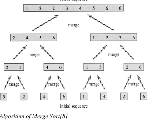
232 2) Merge Sort: The first example of a divide-and-conquer algorithm which we will consider is perhaps the best known. This is a simple and very efficient algorithm for sorting a list of numbers, called MergeSort. We are given an sequence of n numbers A, which we will assume is stored in an array A[1 ...n]. The objective is to output a permutation of this sequence, sorted in increasing order. This is normally done by permuting the elements within the array A. How can we apply divide-and-conquer to sorting? Here are the major elements of the MergeSort algorithm. Divide: Split A down the middle into two subsequences, each of size roughly n/2.

Conquer: Sort each subsequence (by calling MergeSort recursively on each).

Combine: Merge the two sorted subsequences into a single sorted list.

[image:5.612.49.291.444.644.2]

The dividing process ends when we have split the sub sequences down to a single item. An sequence of length one is trivially sorted. The key operation where all the work is done is in the combine stage, which merges together two sorted lists into a single sorted list. It turns out that the merging process is quite easy to implement. The following figure gives a high-level view of the algorithm.

The following figure gives a high-level view of the algorithm.

Algorithm of Merge Sort[8]

1. MergeSort(min,max)

2. If(min<max)

3. Mid (low+high)/2;

4. MergeSort(min,mid);

5. MergeSort(mid+1,max);

6. Merge(min,mid,max);

7. Merge(min,mid,max)

8. h min, i min, j mid+1;

9. while (h<mid) and (j<=max) do

10. if a[h]<=a[j] then

11. b[i] a[h];h h+1;

12. else

13. b[i] a[j];j j+1;

14. i i+1;

15. if h>mid then

16. for k j to max do

17. 10.b[i] a[k]; i i+1;

18. 11. else for k h to mid do

19. 12.b[i] a[k]; i i+1;

20. 13.for k min to max do a[k] b[k];

E. Heap Sort In computer programming, heap sort is a comparison-based sorting algorithm[9]. Heapsort can be thought of as an improved selection sort: like that algorithm, it divides its input into a sorted and an unsorted region, and it iteratively shrinks the unsorted region by extracting the largest element and moving that to the sorted region. The improvement consists of the use of a heap data structure rather than a linear-time search to find the maximum.

Algorithm of Heap sort:

HEAPIFY(A, i)[10]

1 l LEFT(i)

2 r RIGHT(i)

3 if l heap-size[A] and A[l] > A[i]

4 then largest l

5 else largest i

6 if r heap-size[A] and A[r] > A[largest]

(6)

International Journal of Emerging Technology and Advanced Engineering

233 8 if largest i

9 then exchange A[i] A[largest]

10 HEAPIFY(A,largest)

BUILD-HEAP(A)[10]

1 heap-size[A] length[A]

2 for i length[A]/2 downto 1

3 do HEAPIFY(A, i)

HEAPSORT(A)

1 BUILD-HEAP(A)

2 for i length[A] downto 2

3 do exchange A[1] A[i]

4 heap-size[A] heap-size[A] -1

5 HEAPIFY(A, 1).

Given an array of 6 elements: 15, 19, 10, 7, 17, 16, sort it in ascending order using heap sort.

Steps:

Consider the values of the elements as priorities and build the heap tree. Start delete Min operations, storing each deleted element at the end of the heap array. After performing step 2, the order of the elements will be opposite to the order in the heap tree. Hence, if we want the elements to be sorted in ascending order, we need to build the heap tree in descending order - the greatest element will have the highest priority. Note that we use only one array , treating its parts differently:-when building the heap tree, part of the array will be considered as the heap, and the rest part - the original array.when sorting, part of the array will be the heap, and the rest part - the sorted array[11].

Here is the array: 15, 19, 10, 7, 17, 6

Sorting - performing delete Max operations:

1. Delete the top element 19.

1.1. Store 19 in a temporary place. A hole is created at the top

1.2. Swap 19 with the last element of the heap.

As 10 will be adjusted in the heap, its cell will no longer be a part of the heap. Instead it becomes a cell from the sorted array

Percolate down the hole

and this process continue till the end..

2. Store 7 in the hole (as the only remaining element in the heap

(7)

International Journal of Emerging Technology and Advanced Engineering

234 II. PROPOSED METHODOLOGY

We have developed a program in C language to calculate the clock ticks consumed by each algorithm to sort the numbers and also counted the number of swaps taken by each algorithm to generate the sorted list. The elements were randomly generated by using the random function and the clock ticks are counted by using the clock function.

III. SIMULATION/EXPERIMENTAL RESULTS

Sorting algorithms are sometimes characterized by big O notation in terms of the performances that the algorithms yield and the amount of time that the algorithms take, where n is integer. Big O notation describes the limiting behaviour of a function when the argument tends towards a particular value or infinity, usually in terms of simpler functions. Big O notation allows its users to simplify functions in order to concentrate on their growth rates. The different cases that are popular in sorting algorithms are: - O(n) is fair, the graph is increasing in the smooth path.

- O(n^2): this is inefficient because if we input the larger data the graph shows the significant increase. It means that the larger the data the longer it will take.

- O(n log n): this is considered as efficient, because it shows the slower pace increase in the graph as we increase the size of array or data[12]

Table I

COMPLEXITY OF ALGORITHMS

Name Best Case Average Case

Worst Case

Stable

Bubble Sort O(n^2) O(n^2) O(n^2) Yes

Insertion Sort O(n) O(n^2) O(n^2) Yes

Selection Sort

O(n^2) O(n^2) O(n^2) No

Merge Sort O(n log n) O(n log n) O(n log n) Yes Quick Sort O(n log n) O(n log n) O(n^2) No

[image:7.612.323.574.135.299.2]

Heap Sort O(n log n) O(n log n) O(n log n) Yes

Fig.1. Graphical Representation of function

[image:7.612.329.577.506.657.2]

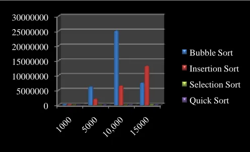
Fig.2 No. of Clock ticks taken by different sorts

0 5000000 10000000 15000000 20000000 25000000 30000000

Bubble Sort

Insertion Sort

Selection Sort

Quick Sort

(8)

International Journal of Emerging Technology and Advanced Engineering

235 IV. CONCLUSION

Based on our experiment, it can be said that for random numbers, quick sort take less time to sort as compare to other algorithms .In other case, worst case complexity of quick sort is O(n^2) which is given by this algorithm when elements are already in sorted order, but for this situation insertion sort give best case complexity. So, at last it can be said that for different situation different sorting algorithms are used but for random numbers quick sort algorithm is chosen.

V. FUTURE SCOPES

In this paper we introduce the comparison of different sorting algorithms based on clock ticks and no. of swaps taken by each sorting algorithm. It produces faster result on that data and it is easy to understand for everyone. It is a straightforward approach and has a lot of future scope. Sorting algorithm based on divide and conquers approach produces very fast result. Theses algorithms are implemented using static data structure, so it may be prospect we will implement using dynamic data structure. At last we want to say there is a vast scope of sorting algorithm in future and to find an optimal sorting algorithm in future.

REFERENCES

[1] Data Structures by Seymour Lipschutz and G A Vijayalakshmi Pai (Tata McGraw Hill companies), Indian adapted edition-2006,7 west patel nagar,New Delhi-110063.

[2] Introduction to Algorithms by Thomas H. Cormen, Charles E. Leiserson, Ronald L. Rivest, fifth Indian printing (Prentice Hall of India private limited), New Delhi-110001.

[3] http://en.wikipedia.org/wiki/Bubblesort. [4] http://en.wikipedia.org/wiki/Insertion_sort.

[5] http://www.programiz.com/article/selection-sort-algorithm-programming.

[6] http://en.wikipedia.org/wiki/Quicksort.

[7] International Journal of Advanced Research in Computer Science and Software Engineering A Comparison Based Analysis of Four Different Types of Sorting Algorithms in Data Structures with Their Performances by Ms. Nidhi Chhajed,Mr. Imran Uddin ,Mr. Simarjeet Singh Bhatia.

[8] Computer Algorithms by Ellis Horowitz, Sartaj Sahni, Sanguthevar Rajasekaran, Galgotia publications,5 Ansari road, Daryaganj, New Delhi-110002.

[9] https://en.wikipedia.org/wiki/Heapsort

[10] https://www.cs.umd.edu/class/fall2006/cmsc351/notes/heapsort [11] http://faculty.simpson.edu/lydia.sinapova/www/cmsc250/LN250_W

eiss/L13-HeapSortEx.htm.