www.hydrol-earth-syst-sci.net/13/749/2009/ © Author(s) 2009. This work is distributed under the Creative Commons Attribution 3.0 License.
Earth System
Sciences
A Bayesian approach to estimate sensible and latent heat over
vegetated land surface
C. van der Tol1, S. van der Tol2, A. Verhoef3, B. Su1, J. Timmermans1, C. Houldcroft3, and A. Gieske1 1ITC International Institute for Geo-Information Science and Earth Observation Hengelosestraat 99, P. O. Box 6, 7500 AA Enschede, The Netherlands
2Delft University of Technology, Faculty of Electrical Engineering, Mekelweg 4, 2628 CD Delft, The Netherlands 3The University of Reading, Department of Soil Science, School of Human and Environmental Sciences,
Reading RG6 6DW, UK
Received: 29 January 2009 – Published in Hydrol. Earth Syst. Sci. Discuss.: 16 March 2009 Revised: 13 May 2009 – Accepted: 21 May 2009 – Published: 12 June 2009
Abstract. Sensible and latent heat fluxes are often calcu-lated from bulk transfer equations combined with the energy balance. For spatial estimates of these fluxes, a combination of remotely sensed and standard meteorological data from weather stations is used. The success of this approach de-pends on the accuracy of the input data and on the accuracy of two variables in particular: aerodynamic and surface con-ductance. This paper presents a Bayesian approach to im-prove estimates of sensible and latent heat fluxes by using a priori estimates of aerodynamic and surface conductance alongside remote measurements of surface temperature. The method is validated for time series of half-hourly measure-ments in a fully grown maize field, a vineyard and a forest. It is shown that the Bayesian approach yields more accurate es-timates of sensible and latent heat flux than traditional meth-ods.
1 Introduction
Sensible and latent heat (i.e. evapotranspiration) fluxes be-tween the land surface and the atmosphere are important components of the land surface energy balance. Different techniques exist to estimate them, generally based on mi-crometeorological methods, including the eddy-covariance, Bowen ratio technique and bulk transfer equations, for ex-ample. Alternatively, estimates of evapotranspiration can be obtained from the soil water balance (see e.g. Verhoef and
Correspondence to: C. van der Tol (tol@itc.nl)
Campbell, 2005, for an overview of both types of methods), from which sensible heat flux could be derived, if values of net radiation and soil heat flux were available.
Field scale measurements are used to study the local wa-ter and energy balance and to gain process understanding, but they are often not representative of large areas. Remote sensing measurements provide a spatial coverage, but not all variables needed to estimate sensible and latent heat can be measured by remote sensing.
It is common practice to combine remote sensing and field data to estimate sensible heat,H, and latent heat flux,λE, spatially (e.g. Su, 2002; Kustas et al., 2007; Anderson et al., 2008). Remote sensing products used as input include bright-ness temperature and emissivity (Bastiaanssen et al., 1998), reflected shortwave radiation and NDVI, which are used for the derivation of vegetation structure and aerodynamic re-sistance (Su, 2002). Weather station variables include wind speed, air temperature and humidity. Latent heat flux is ei-ther solved as a residual term in the energy balance, with
H obtained from a bulk transfer equation or directly calcu-lated using the bulk transfer equation for latent heat flux. The problem with the latter approach, however, is that estimates of specific humidity at the land surface are hard to obtain.
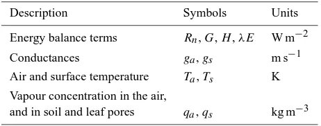
Table 1. Parameters and variables in the energy balance and bulk transfer equations (Eqs. 1 to 3).
Description Symbols Units
Energy balance terms Rn,G,H,λE W m−2
Conductances ga,gs m s−1
Air and surface temperature Ta,Ts K
Vapour concentration in the air,
and in soil and leaf pores qa,qs kg m−3
Quantification of the uncertainty is an essential part of sur-face energy balance modelling. One of the techniques to handle uncertainty of data is data assimilation (Troch et al., 2003). Data assimilation makes it possible to quantify un-certainty, and to find the best solution of a model given vari-ous sources of input data with associated errors. Time series used for surface energy balance modelling are often incom-plete, and data are collected at different spatial scales. In such cases, data assimilation is a useful technique. It has been used to improve the predictions of hydrological mod-els (Schuurmans et al., 2003), to retrieve spatial and tempo-ral trends in root water extraction by vegetation from remote observations of surface temperature and ancillary data (Crow and Wood, 2003), and to retrieve (simulated) soil moisture by model inversion (Reichle et al., 2002).
This paper presents a data assimilation approach to esti-mate sensible and latent heat flux over vegetated land surface. The data used to test the approach include remotely measured surface temperature in conjunction with ground-based mete-orological measurements. In principle, the metemete-orological data are sufficient to calculate sensible and latent heat flux. This makes it possible to calculate the energy fluxes even in the absence of surface temperature measurements, for exam-ple between satellite overpasses or during cloudy conditions. By adding remote measurements of surface temperature (by means of data assimilation), the estimates of the fluxes are improved, because information is added to the model. This approach has already been suggested by Franks et al. (1999). A simple form of data assimilation is used in this paper: the Bayesian theorem described in statistical handbooks (e.g. Carlin and Louis, 1996).
In Sect. 2.1 we first present the energy balance model, bulk transfer equations, and discuss classic approaches to estimate evapotranspiraton (Sect. 2.2). Next, the Bayesian theorem is explained in detail (Sect. 2.3). Furthermore in Sect. 3 it is de-scribed how the data are used to test the Bayesian approach, and the field experiments are described. We finish with the results and discussion in Sects. 4 and 5, respectively.
2 Theory
2.1 Energy balance
The standard energy balance equation is used, consisting of four components: net radiation,Rn, soil heat flux,G, sen-sible heat flux, H and latent heat flux, λE (all in W m−2). Energy involved in melting and freezing or in chemical re-actions, energy stored in the canopy, and energy horizon-tally transported by advection are ignored. Hence (Brutsaert, 2005):
Rn−G=H+λE (1)
Parameterλis the latent heat of evaporation of water (J kg−1)
andEthe evapotranspiration rate (kg m−2s−1).
Sensible and latent heat flux are the fluxes of heat and wa-ter vapour between the surface and the atmosphere carried by turbulent air flow. They are calculated as the product of a conductance and a driving force between the surface (sub-script “s”) and the air at measurement height (subscript “a”), often called “bulk-transfer equations”:
H =ρcpga(Ts−Ta) (2)
λE=λ 1
1/ga+1/gs (qs(Ts)−qa) (3)
whereρis the mass density of air (kg m−3),cpthe heat ca-pacity of air (J kg−1K−1), ga is the aerodynamic conduc-tance (m s−1)for transport of heat and vapour from the sur-face boundary layer into the atmosphere, gs (m s−1)is the
surface conductance for water vapour transport from stom-atal cavities in leaves or soil pores, to the leaf or soil surface boundary layer,Ts is surface temperature andTais air
tem-perature (both in K),qs is the vapour concentration in
stom-ata or soil pores (kg m−3), andqais the vapour concentration
in the air (kg m−3).
Equations (1) to (3) contain 13 parameters and variables. Three of them can be considered constant or can accurately be estimated (ρ, cpandλ). Out of the other 10 (Table 1), at
least 7 need to be measured or estimated in order to solve the three equations. Weather station data are commonly used for the driving variables, such asTa,qaor wind speed (required
for calculation ofra); insofar they are representative for the
area under study.
The surface conductance and the aerodynamic conduc-tance are particularly difficult to estimate.
Surface conductance,gs, of individual leaves can be
Leuning, 1995). These relationships require vegetation-specific, a priori coefficients or local calibration against mea-sured fluxes of water and carbon dioxide. However, for many applications these models are too detailed, as parameters for the vegetation under study are often not available.
The aerodynamic conductance, ga, depends on the
mo-mentum and scalar roughness length of the surface,z0M(m) andz0H(m), respectively, wind speedu(m s−1), and stabil-ity of the atmosphere, as combined in the logarithmic wind profile (Tennekes, 1973; Garratt, 1992). The momentum roughness length, z0M, is usually estimated from leaf area index and vegetation height (e.g. Raupach, 1994; Verhoef et al., 1997a), whereas the scalar roughness length,z0H, is of-ten taken as a constant fraction ofz0M; this fraction varies widely, largely depending on canopy density (Stewart et al., 1994; Verhoef et al., 1997b). Optical remote sensing is often used to estimate vegetation height and leaf area index (Su, 2002). However, estimates of aerodynamic resistance based on optical remote sensing contain a large degree of uncer-tainty.
Apart from the aerodynamic and surface conductance, the difference between surface and air temperature (Ts−Ta) is
also difficult to estimate. Sensible heat flux is proportional to this difference; a relatively small difference between two measurements. WhenTs is taken from remote sensing and Ta from weather station data, then errors in eitherTs orTa
may cause significant errors in the estimates ofH.
2.2 Classic approaches to estimate evapotranspiration
The difficulty in estimatingga,gs and (Ts−Ta), in Eqs. (1)
to (3) has been overcome in a number of ways. This has resulted in three techniques to calculate evapotranspiration from the energy balance:
1. FAO-approach: evapotranspiration is calculated by multiplying a “reference evapotranspiration” by an em-pirical coefficient for a specific crop, extracted from a table based on expert knowledge. The reference evapo-transpiration is calculated for a crop with known values for ga and gs, usually the typical short, well-watered grass of a meteorological station. This method is dis-seminated by the FAO (Allen et al., 1998, 2006), and is mainly used to calculate irrigation requirements. 2. Ts-approach: evapotranspiration is calculated by
solv-ing Eqs. (1) to (3) withH, λE and gs as unknowns.
In that case, on top of the standard meteorological vari-ables, surface temperature measurements and estimates of aerodynamic conductancegaare required. This
tech-nique is used in remote sensing, for example in the model SEBS (Su, 2002). Surface temperature is re-trieved from thermal remote sensing, and aerodynamic resistance from optical remote sensing.
3. Conductance-approach: evapotranspiration is calcu-lated by solving Eqs. (1) to (3) with H, λE and Ts
as unknowns. Aerodynamic conductance is estimated from a measured wind profile or from a priori values for a specific vegetation type, and surface conductancegs
is estimated with one of the combined photosynthesis-conductance or empirical models discussed above. Val-ues for the parameters of such models are found from calibration of the model against measurements ofgs or
taken from the literature.
2.3 Bayesian approach
The Bayesian approach used in this paper, as an alternative to the classic approaches described in Sect. 2.2, combines the methods (2) and (3) discussed above. In the Bayesian ap-proach, neither a real distinction between “knowns” and “un-knowns” is made, nor a distinction between “variables” and “parameters”. The distinction is rather between “a priori” variables and parameters (values for parameters and vari-ables that were measured, estimated, or taken from the lit-erature), and “posterior” values (most likely values for pa-rameters and variables, taking into account all a priori values and their uncertainty, and using the model). A priori values are indicated with a tilde (∼) placed above a symbol. Pos-terior values are indicated with a hat (ˆ). The “real” values, which are never known, do not have a superscript.
It is now assumed that besidesρ,cpandλ, alsoTa,qa,Rn
andGare accurately measured, such that their uncertainty can be ignored. Forga,gs andTs, uncertain, a priori esti-mates are used, and for qs, the saturated humidity atTs is used. No a priori information about the fluxesH andλE
is used. Doing so results in three equations (Eqs. 1 to 3) with two unknowns (HandλE), which implies that the en-ergy balance is over-specified. Theoretically, Eq. (1) is not no longer strictly necessary (we could estimate the fluxes without using Eq. 1), but in doing so we abandon the phys-ically realistic and useful constraint of energy balance clo-sure. Similarly, we could calculate the fluxes without using measuredTs (as in the conductance-approach), but in doing
so we ignore part of the data that we have available. Finally, we could calculate the fluxes without using a priorigs(as in theTs-approach), but in doing so we ignore that gs is lim-ited to physically realistic bounds. The fact that the model is over-specified is not a problem, since the values forga,gs
andTs are not fixed but uncertain. They will be adjusted, resulting in posterior values.
In theTs-approach of Sect. 2.2, all uncertainty of the
mea-surements propagates into the unknowngs, which may lead
to unrealistic values forgs. Similarly, in the
conductance-approach of Sect. 2.2, all uncertainty of the measurements propagates into the unknownTs, which may lead to
unrealis-tic values forTs. In the Bayesian approach, all three
values for any of them are avoided. It is expected that this also leads to more accurate estimates of the fluxesH and
λE.
The model (Eqs. 1 to 3) is re-written such thatTsis output
of the model, by eliminatingH andλEfrom Eqs. (1) to (3) and writingTs as the dependent variable. In other words,Ts
is a function of all input variables and parameters. Hence: ˜
x=f (θ˜)+w (4)
wherex˜ represents the measured output (in this case mea-suredTs),fthe model equations,θ˜a vector of a priori values
of variables and parameters, andwbackground noise caused by the uncertainty of the model and measurements. Note that Eq. (4) could be expressed in terms of the parameters of Eqs. (1) to (3) explicitly, but this would result in a rather long expression. The vector notation is used if the problem is solved for multiple time steps, multiple pixels, or for mul-tiple measurements and parameters. This aspect is discussed later in this paper.
Parameter values (gaandgs)have an a priori probability density functionp(θ), and measurements ofTs a probabil-ity densprobabil-ity functionp (x˜θ). Note thatga andgs are vari-ables. In this study we will calculate them for each time step independently. For an individual time step, ga andgs can
be considered as model parameters. The probability den-sity function of the parameter values is determined by the accuracy of a priori estimates, whereas the probability den-sity function of the measurements ofTs is determined by the
accuracy and representativeness of the measurements. The implementation of these probability density functions for the data used in this study is discussed in Sect. 3. The poste-rior probability density of the parameters (i.e. the parameter values, given the measurements ofTs), is calculated with the classic Bayes’ theorem (Carlin and Louis, 1996):
p(θ|x˜)= p (x˜
θ)·p(θ) R
p (x˜θ)·p(θ)dθ
(5) The numerator in Eq. (5) is a multiplication of the two prob-ability density functions, whereas the denominator is a nor-malization term. A low probability of a value forTs (aTs
that deviates significantly from the measured value), or a low probability of a value for the parameters (a conductance that deviates significantly from the a priori value), results in a low probability of the posterior parameter values. The ex-pected values of the parameters are given by the minimum least square error estimate of the parameters. These expected values can be calculated by integrating the probability den-sity function:
θ=E(θ|x˜)=
Z
θ·p θ|x˜
dθ (6)
The expected values are the posterior (or the optimum) values for the parameters. The posterior values are the weighted average (weighted over their probability) of all pos-sible parameter values. The integration in Eq. (6) is avoided
by calculating only the peak of the probability density func-tion:
_
θ =arg max
θ
p(θx˜)=arg min
θ
(7)
Cx
−1/2 f (θ)−x˜ 2
+ C
−1/2
θ (θ−θ0)
2
where Cx and Cθ are the covariance matrices for the
mea-surements and the parameters, respectively. Parameters_θare the posterior parameter values forgaandgsused later to
cal-culate sensible and latent heat flux.
The last part of Eq. (7) (between the brackets) is a cost function or the quadratic error. The quadratic error is the sum of two components: the quadratic error in the parameters (θ) scaled with the uncertainty of the a priori estimates, and the quadratic error in the measurements ofTs, scaled with the
uncertainty of the measurements ofTs. The optimum
param-eter values are located at the minimum total error. If both
p(x˜|θ)and p(θ) are Gaussian, then the solution is exact (and Eqs. (6) and (7) will give equal results), otherwise it is an approximation. In this study, Gaussian distributions for both functions are assumed.
The key issues are to estimate a priori values of θ, and to estimate the two covariance matrices. These matrices de-scribe the uncertainty of all input (measurements and the a priori values), and determine the contribution of different in-put variables to the posterior estimates. These issues are ad-dressed in detail in Sect. 3.1.
3 Methodology
3.1 Model input
The Bayesian approach is applied using meteorological time series for three land cover types: maize, a vineyard and a for-est, measured during intensive field campaigns (Sect. 3.2). Measured values of four variables are directly used as input for the model: Rn,G,Ta, andqa. It is assumed that these
values were accurately measured and that the measurements were representative of the land cover (Rn= ˜Rn, etc.). This
implies that for these four variables, a priori and posterior values are equal to each other. In contrast, uncertainty is at-tributed to the other variables,ga,gsandTs. Posterior values
forga,gsandTswere calculated with the Bayesian approach
(Eq. 7). The posterior values were used to calculate sensible and latent heat fluxes with Eqs. (1) to (3). Measured sensible and latent heat fluxes were used for validation only.
It is necessary to estimate the a priori values forgaandgs, as well as the uncertainty of a prioriga,gs andTs. Hence, the following equations forga,gsandTs are introduced:
ga=θ1u=
˜
θ1+w1
u (8)
gs =θ2= ˜θ2+w2
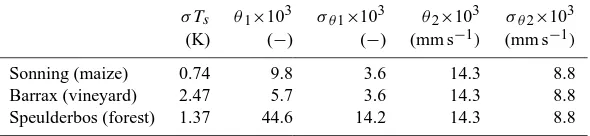
Table 2. A priori values forθ1andθ2, and standard deviations forθ1,θ2andTs.
σ Ts θ1×10³ σθ1×10³ θ2×10³ σθ2×10³
(K) (−) (−) (mm s−1) (mm s−1)
Sonning (maize) 0.74 9.8 3.6 14.3 8.8
Barrax (vineyard) 2.47 5.7 3.6 14.3 8.8
Speulderbos (forest) 1.37 44.6 14.2 14.3 8.8
where w indicates noise, θ1 is a dimensionless parameter which includes the effects of surface roughness and stabil-ity of the boundary layer,uis wind speed (m s−1), and pa-rameterθ2is surface conductance (m s−1). The expression for ga is an additional model, that enables us to estimate
aerodynamic conductance a priori (gais a function of wind
speed). The a priori estimate for parameterθ1 for neutral conditions is calculated using the logarithmic wind profile following Tennekes (1973) and Goudriaan (1977):
˜
θ1=
κ2
lnzz−d
0M
lnzz−d
0H
(9)
whered=0.67h,z0M=0.13h,z0H=0.1z0M,his the vegetation height,zthe measurement height of wind speed (all in m), andκ(=0.4) is Von K´arm´an’s constant. Equation (9) does not include a correction term for non-neutral atmospheric condi-tions. For the a priori estimate of parameterθ2, the FAO stan-dard value for short, well watered grass ofgs=0.0143 m s−1
is used for all three study sites. Values forT˜s are computed
from Stefan-Boltzman equation, using measured outgoing longwave radiation and an emissivity of 0.98. For the forest site, no reliable measurements of outgoing longwave radia-tion were available. For this site, surface temperature was measured with small Negative Temperature Coefficient ther-mistors (NTC) attached to needles (referred to as “contact temperatures” in this paper).
The uncertainty of the a priori estimates and measure-ments, which determine the matrices Cxand Cθ in Eq. (7),
are estimated as follows. It is assumed that the probability of
θ1,θ2andTs have normal distributions with a standard
de-viation of one quarter of the difference between their upper and lower limits found in the literature. The upper and lower limit ofθ1for crops (in this case maize and vineyard) and for forest are based on minimum and maximum values for
z0Mreported in a review paper of Garratt (1993). For these extreme values ofz0M, corresponding extreme crop heights (h=z0M/0.13) and zero plane displacement height (d=2/3h)
are calculated. The upper and lower limits ofθ1 are calcu-lated from the corresponding values ofz0M,z,handd with Eq. (9). An empirical equation forgs of Allen et al. (1998) is used to estimate the upper and lower limits ofθ2:
gs =
LAIactive
100 (10)
where LAIactive is the leaf area index (m2leaf m−2surface) that contributes to transpiration. For the upper and lower lim-its ofθ2(i.e.gs), the values corresponding to a LAIactiveof
3.5 and 0 are used, respectively. The upper and lower limits ofTs are estimated by applying Stefan-Boltzmann equation for two extreme values of emissivity (0.90 and 0.99 for the vineyard and 0.95 and 0.99 for the fully grown maize). For the forest site, the standard deviation of the readings of nine thermistors is used as a proxy for the standard deviation of
Ts. Table 2 presents the a priori values and standard
devia-tionsσθ1,σθ2andσT sderived in this way.
It is further assumed that the covariances (cov(θ1, θ2), cov(θ1,Ts), cov(θ2,Ts))are zero, and that the errors inθ1, θ2andTsof consecutive time steps of a time series are
uncor-related. The latter assumption may not be realistic: estimates of roughness parameters and surface temperature measure-ments may be biased and errors inθ1 andTs are therefore most likely to be similar for consecutive time steps. How-ever, it appears that reasonable results can be obtained even when these effects are ignored. Assuming that all covari-ances are zero makes it possible to solve Eq. (7) for every time step individually. This is computationally more effi-cient than solving Eq. (7) for the whole time series at once, which requires manipulation of large matrices containing the parameters of all (half-hourly) time steps.
The posterior parameters for an individual time step are now calculated with Eq. (7), using:
θ=
θ1
θ2
and θ0= ˜
θ1 ˜
θ2
(11)
Cθ =
σθ21 0 0 σθ22
and Cx=σT s2 (12)
Ts-approach, using Eqs. (1) to (3) withH,λEandgs as un-knowns, and using the a priori expression for ga (ga= ˜θ1u) and measuredTs; and Method 3: the conductance-approach, using Eqs. (1) to (3) withH,λEandTs as unknowns, and
using a priori values forgaandgs.
3.2 Experimental setup
The Bayesian approach is applied using micrometeorologi-cal time series obtained for a maize crop (Sonning, UK), a vineyard (Barrax, Spain) and a Spruce forest (Speulderbos, The Netherlands). For the maize crop, 9 days, for the vine-yard, 6 days and for the forest, 3.5 days worth of half-hourly data are used.
3.2.1 The maize field
Meteorological input variables and fluxes were obtained over a fully grown maize field (row spacing was 0.75 m, the within-row spacing was about 0.12 m) located at the Crops Research Unit at Sonning farm (a research facility owned by the University of Reading, UK). It is located 4 km from Reading in Sonning (UK), at 51.48◦N, 0.90◦W, elevation 35 m above sea level (see Houldcroft, 2004); the soil type is loamy sand. Data from 7 to 16 September 2002 were used, when the leaf area index was 3.4 m2m−2 and the canopy height 1.9 m.
Net radiation was measured using a CNR1 four-component net radiometer (Kipp and Zonen, Delft, The Netherlands) at a mounting height of 2.5 m above the ground. Soil heat flux was calculated using a Fourier analysis on mea-sured soil temperatures, combined with estimates of thermal diffusivity and heat capacity, the so-called analytical or exact method (see e.g. Verhoef, 2004). The soil temperatures were acquired with type-NT 10 kthermistors (RS, UK) that had been encapsulated with a stainless steel housing, accuracy of±0.2◦C, installed at nominal depths of 2 and 5 cm. Soil heat flux at the surface (z=0), i.e.G, was calculated by us-ing a negativez(i.e.−0.02 m) in the analytical equation of soil heat flux. Thermal diffusivity was calculated using the Arctangent method (Verhoef et al., 1996), using soil temper-ature signals at both depths, and heat capacity was calculated from the soil moisture content at 5 cm depth, measured using a Thetaprobe (Delta-T Devices).
Wind speed was measured using an AN1 cup anemometer (Delta-T Devices, UK), air temperature and humidity were measured with a RHT2 psychrometer, all at a height of 4 m above the surface. Surface temperature was estimated by inverting Stefan-Boltzmann’s law, using outgoing longwave radiation measured with the CNR1 radiometer and an emis-sivity of 0.98. Although contact temperature measurements of the surface were available as well, these were not used in order to approximate remote sensing measurements as much as possible.
Sensible and latent heat fluxes were obtained using a com-bination of a Solent R3 sonic anemometer (Gill Instruments Ltd, Lymington, Hampshire, UK) and a differential closed-path infrared gas analyser (LI-7500, LICOR Inc., Lincoln, NE, USA), with appropriate correction procedures applied. 3.2.2 The vineyard
Meteorological input variables and fluxes were obtained over a vineyard (row spacing was 3.35 m, the within-row spacing was approximately 1.5 m, LAI was 0.52 m2m−2, fractional vegetation cover 0.33 and vegetation height about 2 m) lo-cated at the Barrax agricultural test site in Spain (39.06◦N, 02.10◦W), where various crops were grown, some of them irrigated. Data were collected between 14 and 21 July 2004 during an intensive field campaign (SPARC). The experiment has been described in detail by Su et al. (2008).
Net radiation was measured using a CNR1 four-component net radiometer at a mounting height of 4.8 m above the ground. Soil heat flux was measured with 3 Hukse-flux HFP01 heat Hukse-flux plates (Campbell Scientific Inc., USA) at 0.5 cm depth. Heat storage above the sensors was ne-glected. Air temperature and relative humidity were mea-sured with a HMP45 sensor (Vaisala, Finland) at 4.78 m height, wind speed with a cup anemometer (Vector Instru-ments, Ltd., United Kingdom) at 4.88 m height. Surface tem-perature was estimated by inverting Stefan-Boltzmann’s law, using outgoing longwave radiation measured with the CNR1 radiometer and an emissivity of 0.98. All data were collected at 1 min intervals, and 10-min averages were stored, and half hourly averages were used in this study.
Sensible and latent heat fluxes were obtained using a com-bination of a Solent R3 sonic anemometer (Gill Instruments Ltd, Lymington, Hampshire, UK) and a differential closed-path infrared gas analyser (LI-7500, LICOR Inc., Lincoln, NE, USA) installed at 3.4 m height. Further details about the experiment can be found in Timmermans et al. (2009). 3.2.3 The forest
Meteorological input variables and fluxes were obtained over a Douglas fir stand planted in 1962 in the Veluwe forest ridge in the Netherlands (52.50◦N, 05.69◦E). The research site is equipped with a 47 m high measurement tower maintained by the Dutch National Institute for Public Health and the En-vironment (RIVM). The tree density is 785 trees per hectare and the tree height 32 m. Leaf area index is approximately 5 m2m−2. The topography is slightly undulating with height variations of 10 to 20 m within distances of 1 km. Data were collected between 10 and 21 June 2006 during an intensive field campaign (EAGLE). Details about the field campaign are described by Su et al. (2009).
plates at 0.5 cm depth below the litter layer. Temperature, humidity and wind speed were measured at 35 m height. Be-cause of an issue with the CNR1 radiometer (the temperature of the instrument was not correctly measured), the outgo-ing longwave radiation could not be used to estimate surface temperature. Instead, contact temperatures were measured with Negative Temperature Coefficient (NTC) sensors, 9 of which were attached to needles and branches and 8 placed on the soil. The average temperature of the 9 NTC’s con-nected to the vegetation was used as an estimate of surface temperature. Because of the dense vegetation, the contri-bution of soil temperature was neglected. Contact temper-ature measurements were only available between 15 and 21 June 2006. Meteorological measurements were carried out and data stored at 1 min intervals. Half-hourly averages were used in this study.
Sensible and latent heat flux were measured with a CSAT3 sonic anemometer (Campbell Scientific, USA) and an open path infrared gas analyser (LI-7500, LICOR Inc., Lincoln, NE, USA) installed at 47 m height. The data were processed with the software package ECpack (http://www.met.wau.nl/ projects/jep/index.html) and corrections were carried out ac-cording to Van Dijk et al. (2004).
4 Results
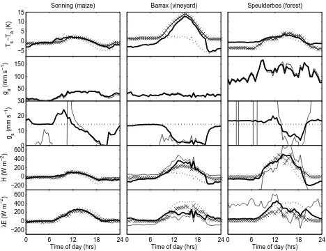
Figure 1 shows plots of a number of key variables versus time, measured and calculated with the three above men-tioned methods, for one example day with clear sky con-ditions, for each of the three field sites. The plotted vari-ables are the difference between surface and air temperature (Ts−Ta), the aerodynamic and surface conductance,ga and
gs, and the sensible and latent heat flux,HandλE.
The concuctance-approach by definition follows the a pri-ori values for both ga andgs, without making use of the
measurements ofTs. For the Barrax site, this approach
re-sults in much lower modelled than measuredTs−Ta. The Ts-approach, by definition, follows the measurements forTs,
irrespective of the corresponding values forgs. The modelled
vales forgsare often outside the range of values found in the
literature, even negative or infinitely high. The Bayesian ap-proach compromises between following measured values for
Ts and following the a priori values for the conductancesga
andgs. The advantage of the Bayesian approach is that, in this way, extreme values ofTs,gaorgs are avoided.
The Bayesian approach has a second advantage: the pos-terior values ofgaandgsreveal actual information about the
surface which is neither present in the a priori values, nor in the model. Posterior aerodynamic conductance ga does
not deviate much from a priori, but surface conductancegs
shows a clear diurnal pattern. The highest values ofgs are
found in the late morning for the maize and the forest. In the afternoon,gs decreases until a minimum at 19:00.
Dur-ing daytime hours, gs at the vineyard is lower than gs at
−5 0 5 10 15
Ts
−T
a
(K)
Sonning (maize)
0 50 100 150
ga
(mm s
−1
)
0 10 20 30
gs
(mm s
−1
)
−200 0 200 400 600
H (W m
−2
)
0 6 12 18 24
−200 0 200 400 600
Time of day (hrs)
λ
E (W m
−2
)
Barrax (vineyard)
0 6 12 18 24
Time of day (hrs)
Speulderbos (forest)
0 6 12 18 24
[image:7.595.311.545.62.242.2]Time of day (hrs)
Fig. 1. Measured and modelled values of (Ts−Ta), aerodynamic
conductancega, surface conductancegs, sensible heat fluxH, and
latent heat fluxλE, versus time. The data represent example days
for a fully-grown maize field in Sonning (UK) on 13 September 2002, a vineyard in Barrax (Spain) on 15 July 2004, and a forest in Speulderbos (The Netherlands) on 16 June 2006. The thin solid
line represents theTs-approach, the dashed line the
conductance-approach, the bold solid line the Bayesian conductance-approach, and the symbol “x” represents a field measurement.
the forest and the maize site. These patterns emerge even though a priori values forgs are constant and equal for all
three sites. The patterns agree with conceptual understand-ing: semi-empirical models often predict a decreasing gs
caused by stomatal closure during the afternoon. The lower
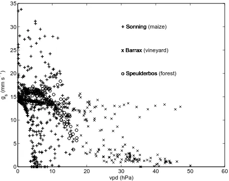
gsfor the vineyard can be explained by the lower vegetation cover (0.33) than that of the other two sites (closed canopies). Figure 2 shows surface conductancegsversus vapour
pres-sure deficit for the four sites. This figure shows a negative correlation betweengsand vapour pressure deficit similar to that described in the literature (e.g. Leuning, 1995).
During the night, due to the small vapour gradient (qs−qa),Ts is relatively insensitive togs. As a result, poste-riorgsreturns to the a priori value during the night. This has little consequences for the calculated fluxes, since these are small during the night.
Figure 1 also shows that the conductance-approach and the Bayesian approach are unable to reproduce night time surface temperatures of the vineyard and the forest. Dur-ing the night, stable, stratified air conditions are formed, in which the aerodynamic conductance strongly reduces (Mass-man and Lee, 2002). We do not find this strong reduction of
gain the posterior values. The reason is that the chosen
0 10 20 30 40 50 60 0 5 10 15 20 25 30 35 vpd (hPa) gs (mm s −1 ) + Sonning x Barrax o Speulderbos + Sonning x Barrax o Speulderbos + Sonning (maize)
x Barrax (vineyard)
[image:8.595.52.285.63.247.2]o Speulderbos (forest)
Fig. 2. Scatter plot of posterior surface conductance versus atmo-spheric vapour pressure deficit (vpd) for all half-hourly data of the three sites.
−100 0 100 200 300 −100 0 100 200 300 H
meas (W m −2) Hmod (W m −2 ) from T s
RMSE = 24 W m−2
−100 0 100 200 300 H
meas (W m −2)
2. from g
a and gs (conductances)
RMSE = 28 W m−2
−100 0 100 200 300 H
meas (W m −2)
3. from T
s, ga and gs (Bayesian)
RMSE = 25 W m−2
0 200 400 −100 0 100 200 300 400 500
λEmeas (W m −2) λ Emod (W m −2 )
RMSE = 47 W m−2
0 200 400
λEmeas (W m −2)
RMSE = 33 W m−2
0 200 400
λEmeas (W m −2)
RMSE = 32 W m−2
Fig. 3. For the maize field (Sonning), for all half-hourly data in the measurement period, modelled versus measured sensible heat
fluxH (upper graphs) and latent heat fluxλE(lower graphs), for
the conductance-approach (left), theTs-approach (middle) and the
Bayesian approach (right).
Concerning the fluxes H and λE, the following is ob-served. The conductance-approach performs well during the night and in the morning, but underestimatesH and overes-timatesλE during the afternoon. The reason is, that the a priori values forgs are constant, and that no stomatal closure
is included in the conductance-approach. TheTs-approach
performs well during the afternoon, but poorly during the night and in the morning. The values of the fluxes calculated with the Bayesian approach always vary between that of a priori and theTs-approach, and closely follow the superior
approach: the conductance-approach in the morning, and the
Ts-approach in the afternoon. Consequently, the Bayesian approach closely follows the measurements.
−100 0 100 200 300 −100 0 100 200 300 H
meas (W m −2) Hmod (W m −2 ) from T s
RMSE = 93 W m−2
−100 0 100 200 300 H
meas (W m −2)
2. from g
a and gs (conductances)
RMSE = 152 W m−2
−100 0 100 200 300 H
meas (W m −2)
3. from T
s, ga and gs (Bayesian)
RMSE = 95 W m−2
0 200 400
−100 0 100 200 300 400 500 λE
meas (W m −2) λ Emod (W m −2 )
RMSE = 121 W m−2
0 200 400
λE
meas (W m −2)
RMSE = 139 W m−2
0 200 400
λE
meas (W m −2)
RMSE = 88 W m−2
Fig. 4. Similar to Fig. 3, but for the vineyard (Barrax).
−100 0 100 200 300 −100 0 100 200 300 H
meas (W m −2)
Hmod
(W m
−2
)
from Ts
RMSE = 362 W m−2
−100 0 100 200 300 H
meas (W m −2)
2. from ga and gs (conductances)
RMSE = 114 W m−2
−100 0 100 200 300 H
meas (W m −2)
3. from Ts, ga and gs (Bayesian)
RMSE = 91 W m−2
0 200 400
−100 0 100 200 300 400 500 λE
meas (W m −2) λ Emod (W m −2 )
RMSE = 351 W m−2
0 200 400
λE
meas (W m −2)
RMSE = 124 W m−2
0 200 400
λE
meas (W m −2)
[image:8.595.306.548.63.244.2]RMSE = 103 W m−2
Fig. 5. Similar to Fig. 3, but for the forest (Speulderbos).
Figures 3 to 5 show the results for the whole measure-ment period as scatter plots of modelled versus measured variables, for the three sites. For all three sites, the Bayesian approach results in the lowest root mean square error for the fluxes. The Bayesian approach reduces both the bias and the scatter compared to the other two approaches.
Both theTs-approach and the Bayesian approach overes-timateλEof the vineyard. This may be caused by an eddy covariance flux measurement error rather than a model error. The vineyard was relatively small and surrounded by bare land, stubble fields and irrigated crops, which contaminated the eddy covariance signal (Timmermans et al., 2009). The high measuredλE values may be attributed to an adjacent irrigated maize field. A different problem with the measure-ments is apparent in the forest, where measuredRnwas 10%
[image:8.595.52.283.300.477.2]forces energy balance closure (Eq. 1), it is possible thatλE
is overestimated, whileH is not underestimated (Fig. 5). It is difficult to reproduce measuredHandλEwhen these measurements are not used for calibration. Obviously, all of the three approaches would perform significantly better if the measured fluxes were used for calibration. However, in practice, measured fluxes are rarely available. Without mea-sured fluxes for calibration, both the conductance-approach and theTs-approach may perform poorly (see, for example,
the conductance-approach in the vineyard (Fig. 3) or theTs
approach at the forest site, Fig. 5). The Bayesian always per-forms better than the other two approaches (a lower RMSE). Moreover, unrealistic parameter values are avoided.
5 Discussion and conclusion
In data assimilation, it is critical to quantify the uncertainty associated to parameters and measurements. This is not al-ways possible for lack of data. A starting point is to identify sources of error. In this particular study, the uncertainties of aerodynamic and surface conductance are relevant.
Dimensionless “aerodynamic” parameterθ1 can vary in space and time for two different reasons: variations in sur-face roughness and variations in atmospheric stability. The first is the dominant cause of variations in space (at a specific time of a satellite overpass), whereas the second is the domi-nant cause of variations in time (at a specific field site). Sim-ilarly, surface conductance, θ2, can vary in space and time for two different reasons: variations in plant species, vegeta-tion density and soil moisture content on the one hand (spa-tial variations) and variations in the diurnal cycle of stomatal regulation on the other hand (temporal variations).
In this study, no distinction is made between sources of error. High standard deviations are used for the two con-ductances in order to cover different errors, although the ef-fect of stability on aerodynamic conductance during the night is not incorporated (see Sect. 4). One may argue that some of the errors are of random nature, whereas others are more constant in time. An approach to handle such differences in the nature of errors is to distinguish between bias and ran-dom noise. This approach has been tested for the data of this study as well, leading to results similar to those presented in this paper.
The simple Bayesian approach led to improved estimates of sensible and latent heat flux of maize, vineyard and for-est compared to more classic approaches which use either measured surface temperature or a priori parameter values. Posterior estimates reveal the diurnal pattern of surface con-ductance during the day (stomatal regulation), without using measured fluxes as input.
Acknowledgements. This research was funded by the Netherlands Institute for Space Research (SRON), project number EO-071. The SPARC and EAGLE campaigns were carried out in the framework of the Earth Observation Envelope Program of the ESA, and
were partly financed by the EU 6FP Project, SRON EO-071, and the ITC International Institute for Geo-Information Science and Earth Observation. The Sonning field campaign was funded by the Natural Environment Research Council (NERC, UK) and a CASE award from the Environment Agency (UK). We thank Dr Bruce Main for his technical assistance in the field. The authors thank Jan Elbers, Wim Timmermans, Remco Dost, and Li Jia for fieldwork and data processing and coordination during the SPARC and EAGLE campaigns, and Wout Verhoef for fruitful discussion. The authors also thank the two anonymous reviewers for their useful comments.
Edited by: J. Wen
References
Allen, R. G., Pereira, L. S., Raes, D., and Smith, M.: Crop evapo-transpiration. Guidelines for computing crop water requirements. FAO Irrigation and Drainage Paper (FAO), no. 56, Rome, Italy, 1998.
Allen, R. G., Pruitt, W. O., Wright, J. L., Howell, T. A., Ventura, F., Snyder, R., Itenfisu, D., Steduto, P. Berengena, J., Yrisarry, J. B., Smith, M., Pereira, L. S., Raes, D., Perrier, A., Alves, I., Walter, I., and Elliott, R.: A recommendation on standardized surface resistance for hourly calculation of reference ETo by the FAO56 Penman-Monteith method, Agr. Water Manage., 81(1–2), 1–22, 2006.
Anderson, M. C., Norman, J. M., Kustas, W. P., Houborg, R., Starks, P. J., and Agam, N.: A thermal-based remote sensing technique for routine mapping of land-surface carbon, water and energy fluxes from field to regional scales, Remote Sens. Envi-ron., 112, 4227–4241, doi:10.1016/j.rse.2008.07.009, 2008 Baldocchi, D. D., Luxmoore R. J., and Hatfield J. L.: Discerning
the forest from the trees: an essay on scaling canopy stomatal conductance, Agr. Forest Meteorol., 54, 197–226, 1991. Ball, J., Woodrow, I., and Berry, J.: A model predicting stomatal
conductance and its contribution to the control of photosynthesis under different environmental conditions in: Progress in photo-synthesis research, Martinus-Nijhoff, The Netherlands, 221–224, 1987.
Bastiaanssen, W. G. M., Menenti, M., Feddes, R. A., and Holtslag, A. A. M.: A remote sensing surface energy balance algorithm for land (SEBAL). 1. Formulation, J. Hydrol., 212–213, 198–212, 1998.
Brutsaert, W.: Hydrology, an introduction, Cambridge University Press, Cambridge, UK, 618 pp., 2005.
Carlin, B. P. and Louis, T. A.: Bayes and empirical Bayes meth-ods for data analysis, Chapman and Hall, London, UK, 399 pp., 1996.
Cowan, I.: Stomatal behaviour and environment, Adv. Bot. Res., 4, 117–228, 1977.
Crow, W. T. and Wood, E. F.: The assimilation of remotely sensed soil brightness temperature imagery into a land surface model using ensemble Kalman filtering: a case study based on ESTAR measurements during SGP97, Adv. Water Resour., 26(2), 137– 149, 2003.
3, 477–488, 1999,
http://www.hydrol-earth-syst-sci.net/3/477/1999/.
Garratt, J. R.: The Atmospheric Boundary Layer, Cambridge Uni-versity Press, UK, 1992.
Garratt, J. R.: Sensitivity of climate simulations to land–surface and atmospheric boundary layer treatments – a review, J. Climate, 6, 419–449, 1993.
Goudriaan, J.: Crop micrometeorology: a simulation study, WAU dissertation no. 683, Wageningen University, The Netherlands, 1977.
Houldcroft, C.: Measuring and modeling the surface temperature and structure of a maize canopy, PhD Thesis, The University of Reading, UK, 2004.
Jarvis, P. O.: The interpretation of the variations in leaf water po-tential and stomatal conductance found in canopies in the field, Philos. T. Roy. Soc. B, 273, 593–610, 1976.
Kustas, W. P., Anderson, M. C., Norman, J. M., and Li, F.: Utility of radiometric–aerodynamic temperature relations for heat flux estimation, Bound.-Lay. Meteorol., 122, 167–187, 2007.
Leuning, R.: A critical appraisal of a combined
stomatal-photoynthesis model for C3 plants, Plant Cell Environ., 18, 339– 355, 1995.
Massman, W. J. and Lee, X.: Eddy covariance flux
correc-tions and uncertainties in long-term studies of carbon and en-ergy exchanges, Agr. Forest Meteorol., 113(1–4), 121–144, doi:10.1016/S0168-1923(02)00105-3., 2002.
Raupach, M. R.: Simplified expressions for vegetation roughness length and zero-plane displacement as functions of canopy height and area index, Bound.-Lay. Meteorol., 71, 211–216, 1994. Reichle, R. H., McLaughlin, D. B., and Entekhabi, D.:
Hydro-logic Data Assimilation with the Ensemble Kalman Filter, Mon. Weather Rev., 130, 103–114, 2002.
Schuurmans, J. M., Troch, P. A., Veldhuizen, A. A., Bastiaanssen, W. G. M., and Bierkens, M. F. P.: Assimilation of remotely sensed latent heat flux in a distributed hydrological model, Adv. Water Resour., 26, 151–159, 2007.
Stewart, J. B., Kustas, W. P., Humes, K. S., Nichols, W. D., Moran, M. S., and De Bruin, H. A. R.: Sensible Heat Flux-Radiometric Surface Temperature Relationship for Eight Semiarid Areas, J. Appl. Meteorol., 33(9), 1110–1117, 1994.
Su, Z.: The Surface Energy Balance System (SEBS) for estima-tion of turbulent heat fluxes, Hydrol. Earth Syst. Sci., 6, 85–100, 2002,
http://www.hydrol-earth-syst-sci.net/6/85/2002/.
Su, Z., Timmermans, W., Gieske, A., Jia, L., Elbers, J. A., Olioso, A., Timmermans, J., Van Der Velde, R., Jin, X., Van Der Kwast,
H., Nerry, F., Sabol, D., Sobrino, J. A., Moreno, J., and Bianchi, R.: Quantification of land-atmosphere exchanges of water, en-ergy and carbon dioxide in space and time over the hetero-geneous Barrax site, Int. J. Remote Sens., 29, 5215–5235, doi:10.1080/01431160802326099, 2008.
Su, Z., Timmermans, W. J., van der Tol, C., Dost, R. J. J., Bianchi, R., G´omez, J. A., House, A., Hajnsek, I., Menenti, M., Magli-ulo, V., Esposito, M., Haarbrink, R., Bosveld, F. C., Rothe, R., Baltink, H. K., Vekerdy, Z., Sobrino, J. A., Timmermans, J., van Laake, P., Salama, S., van der Kwast, H., Claassen, E., Stolk, A., Jia, L., Moors, E., Hartogensis, O., and Gillespie, A.: EA-GLE 2006 – multi-purpose, multi-angle and multi-sensor in-situ, airborne and space borne campaigns over grassland and forest, Hydrol. Earth Syst. Sci. Discuss., 6, 1797–1841, 2009,
http://www.hydrol-earth-syst-sci-discuss.net/6/1797/2009/. Tennekes, H.: The Logarithmic Wind Profile, J.Atmos. Sci., 30(2),
234–238, 1973.
Timmermans, W. J., Su, Z., and Olioso, A.: Footprint issues in scin-tillometry over heterogeneous landscapes, Hydrol. Earth Syst. Sci. Discuss., 6, 2099–2127, 2009,
http://www.hydrol-earth-syst-sci-discuss.net/6/2099/2009/. Troch, P. A., Paniconi, C., and McLaughlin, D. B.:
Catchment-scale hydrological modeling and data assimilation, Adv. Water Resour., 26, 131–217, 2003.
Van Dijk, A., Moene, A. F., and De Bruin, H. A. R.: The princi-ples of surface flux physics: theory, practice and description of the ECPACK library, Internal Report 2004/1, Meteorology and Air Quality Group, Wageningen University, Wageningen, The Netherlands, 99 pp., 2004.
Verhoef, A.: Remote estimation of thermal inertia and soil heat flux for bare soil, Agr. Forest Meteorol., 123(3–4), 221–236, 2004. Verhoef, A., van den Hurk, B., Jacobs A. F. G., and Heusinkveld, B.
G.: Thermal soil properties for vineyard (EFEDA-I) and savanna (HAPEX-Sahel) sites, Agr. Forest Meteorol., 78, 1–18, 1996. Verhoef, A. and Campbell, C. L.: Evaporation Measurement, Ch.
40, in: Encyclopedia of Hydrological Sciences, edited by: An-derson, M. G., John Wiley, Chichester, 589–601, 2005. Verhoef, A., McNaughton, K. G., and Jacobs, A. F. G.: A
pa-rameterization of momentum roughness length and displacement height for a wide range of canopy densities, Hydrol. Earth Syst. Sci., 1, 81–91, 1997a,
http://www.hydrol-earth-syst-sci.net/1/81/1997/.
Verhoef, A., De Bruin, H. A. R., and Van den Hurk, B. J. J. M.:
Some practical notes on the parameter kB−1for sparse canopies,