www.hydrol-earth-syst-sci.net/13/1649/2009/ © Author(s) 2009. This work is distributed under the Creative Commons Attribution 3.0 License.
Earth System
Sciences
Dynamically vs. empirically downscaled medium-range
precipitation forecasts
G. B ¨urger
Universit¨at Potsdam, Institut f¨ur Geo¨okologie, Potsdam, Germany currently at: Pacific Climate Impacts Consortium, Victoria, Canada
Received: 3 April 2009 – Published in Hydrol. Earth Syst. Sci. Discuss.: 27 April 2009 Revised: 25 August 2009 – Accepted: 31 August 2009 – Published: 16 September 2009
Abstract. For three small, mountainous catchments in
Ger-many two medium-range forecast systems are compared that predict precipitation for up to 5 days in advance. One system is composed of the global German weather service (DWD) model, GME, which is dynamically downscaled using the COSMO-EU regional model. The other system is an em-pirical (expanded) downscaling of the ECMWF model IFS. Forecasts are verified against multi-year daily observations, by applying standard skill scores to events of specified inten-sity. All event classes are skillfully predicted by the empirical system for up to five days lead time. For the available predic-tion range of one to two days it is superior to the dynamical system.
1 Introduction
Medium-range prediction of heavy rainfall for flash-flood prone areas such as small mountainous river catchments be-longs to the most important challenges of current weather forecasting. Progress in that field is obviously quite bene-ficial for any affected community, since early warnings in the time frame of several (3–5) days could initiate protec-tion measures and thus avoid much of the damage that is usually brought about by flash floods. Medium-range pre-dictability comes mainly from numerical weather prediction (NWP), where general circulation models (GCMs) simulate the global atmosphere several days into the future. But phys-ical and numerphys-ical conditions impose a limit on the spa-tial resolution of GCMs, rendering their direct output fairly useless for many practical applications. Additional steps are therefore needed to derive small-scale information from GCMs.
Correspondence to: G. B¨urger ([email protected])
This “downscaling”-named procedure exists in two forms, dynamical and empirical, both of which have their advan-tages and disadvanadvan-tages. The main advantage of the dynam-ical approach is the foundation on first principles, which re-quires only a limited number of additional, empirically de-rived parameters to represent the unresolved scales. But the complex interplay between model dynamics and topography is difficult to represent physically so that, e.g., positional errors sometimes slip in. This problem is not encountered in empirically based methods as they are directly calibrated against the observed climate, and any potential bias should in principle be removed by the calibration. But to do so re-quires a considerable amount of parameters that are hard to estimate with sufficient confidence, and that introduces extra errors in the forecasts. But once these parameters are esti-mated, empirical model forecasts are usually much cheaper numerically.
Fig. 1. The three river basins.
I am not aware of any systematic comparison between dy-namical and empirical methods of NWP downscaling. In this study, daily precipitation forecasts are compared that are made by two coupled systems for three small head catch-ments in Germany. One system is the Globalmodell (GME) downscaled by the Lokalmodell (LM, now COSMO-EU) of the German weather service (Majewski et al., 2002; Damrath et al., 2000). The other is the Integrated Forecast System (IFS) of the European Centre for Medium Range Weather Forecast (ECMWF), empirically downscaled using expanded downscaling (EDS) (White, 2002; B¨urger, 1996). The sys-tems are compared with regard to three intensity classes, by verifying binary forecasts of the corresponding events using standard scores.
2 Data and methods
2.1 The catchments
Atmospheric flow over Germany is westerly dominated, with blocking intermezzos that redirect winds northward or south-ward. The interplay between this flow and the orography of a catchment leads to typical precipitation characteristics. For example, while Alb and Upper Danube are in close proxim-ity one (Alb) is located west and the other east of the Black Forest, giving them typical luv–lee characteristics with cor-responding climate. The Upper Iller, on the other hand, is
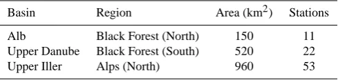
Table 1. The three study areas.
Basin Region Area (km2) Stations
Alb Black Forest (North) 150 11
Upper Danube Black Forest (South) 520 22
Upper Iller Alps (North) 960 53
located just North of the Alps and receives the greatest pre-cipitation amounts during northerly (blocking) flow. Fig-ure 1 displays the location of the three catchments in South-ern Germany. Their main characteristics are summarized in Table 1.
For each basin, average precipitation over all reporting sta-tions will be verified. Although varying availability of data reduces verification performance through time, each forecast system is affected equally so that a fair comparison is possi-ble.
2.2 The GME/LM forecasting system
Unlike most other GCMs, the GME employs a gridpoint ap-proach of a icosahedral–hexagonal type, with an almost uni-form mesh size for the entire globe (i.e. without grid con-vergence at the poles). Until 27 September 2004, that size was∼60 km with 31 levels, and it changed to∼40 km and 40 levels afterwards. The model is initialized in a 3 h time interval using a data assimilation scheme that is based on optimum interpolation. Forecasts up to+174 h are issued twice daily at 0:00 and 12:00 UTC, with an additional+48 h forecast issued at 18:00 UTC. Details of the model can be found in (Majewski et al., 2002). The regional model LM is a non-hydrostatic model that operates on 35 levels and a grid spacing of 7 km covering central Europe. When nested in the GME it receives initial and boundary conditions from that model.
For this study, GME/LM forecasts were available from 2002 to 2005, issued daily at 12:00 UTC for lead times of +12 h,+24 h,+36 h,+48 h. The verified quantity was av-erage precipitation of all grid points covering the catchment area.
2.3 The IFS/EDS forecasting system
[image:2.595.308.553.97.155.2]levels throughout. (Later in 2006 the system was once more upgraded toTL399 or∼50 km, and 62 levels.) For the sub-sequent downscaling the following fields were selected from the 850 hPa level:
– geopotential height
– temperature
– vorticity
– specific humidity
And from the surface level
– total precipitation
was included as a fifth predictor field. All fields were inter-polated on a 1×1 degree grid, using the rectangular section between the edges (4◦W, 46◦N) and (18◦W, 56◦N), which roughly covers the area of central Europe. Concatenation of all fields results in an array of dimension 825=5×(15×11). By applying an empirical orthogonal function (EOF) anal-ysis and retaining only the most dominant EOFs it is pos-sible to reduce this dimension considerably. The reduction should keep as much of the field’s fine structure as is neces-sary to represent, e.g., the major floods of concern, but not so much that one ends up fitting noise. In this case, retain-ing 81 EOFs was a good compromise (as further discussed in Sect. 4). It should be noted that by using the entire synoptic domain (here central Europe) the downscaling must not be confused with a simple MOS approach.
The study covers the decade from 1997 to 2005. Even for the highest available EPS resolution of about 80 km the size of the Alb basin (150 km2) is only about 3% of the size of one grid cell (6400 km2), so the need for downscaling is obvious. The IFS forecasts are issued at 12:00 UTC. For to-tal precipitation (as an accumulating quantity) and a forecast lead time of +lh, l=0,12, . . . ,120, the overlapping 24 h-sums of(l+24)h−lh were used as predictor (local precipi-tation is observed in 24 h-sums only).
Suppose the series of daily atmospheric predictors is given
asx(t )=(x1(t ), . . . , xn(t )), withn=81. On the other hand,
let all station variables be concatenated to form the sin-gle vector time seriesy(t )=(y1(t ), . . . , ym(t )); in our case,
m=11. I assume that both series have been transformed to
N (0,1)-variates (normal with zero mean and unit variance) using the probit transformation (Ledermann et al., 1984; B¨urger, 1996). This will ensure that all scales are weighted adequately by the EDS model, to be described now.
With one exception, the EDS model is just like multiple linear regression (MLR). For both one assumes a model
y=xQ+ε, (1)
which has MLR as the least squares solution MLR=argmin
Q
kxQ−yk (2)
(k · kdenoting the Frobenius norm). The problem with MLR is that the simulated amplitudes are scaled by the prevailing canonical correlations betweenxandy, and are thus damped relative to observations (B¨urger et al., 2006). By imposing onQthe side condition that local covariance be preserved one obtains as a solution the expanded downscaling (EDS) matrix:
EDS=argmin Q
kxQ−yk, subj.to Q0x0xQ=y0y.(3)
Equation (3) describes a so called nonlinear programming problem which is numerically very complex and hard to im-plement. But recently the following closed-form solution of Eq. (3) was found (B¨urger et al., 2009):
EDS=G−x1V U0Gy (4)
HereGxandGydenote the Cholesky factors ofx0xandy0y, respectively, andUandV are from the singular value decom-position
U6V0=Gyy0xG−x1. (5)
Accordingly, when driven by global fields that have identi-cal covariance to the identi-calibrating fields of EDS, the simulated local record has covariance identical to the observed record. EDS is optimal among all linear maps with this property, by leaving the smallest possible error in Eq. (1). It was orig-inally developed for the downscaling of climate scenarios, with particular emphasis on hydrologic extremes (B¨urger, 2002; Menzel et al., 2006).
Mar-12 Mar-17 Mar-22 Mar-27 2002
0 20 40 60
areal P [mm/d]
OBS IFS/EDS GME/LM
Sep-28 Oct-03 Oct-08 Oct-13
2003 0
20 40 60
areal P [mm/d]
Jan-06 Jan-11 Jan-16 Jan-21
2004 0
20 40 60
areal P [mm/d]
Jan-10 Jan-15 Jan-20 Jan-25 Jan-30
2005 0
20 40 60
[image:4.595.71.516.62.352.2]areal P [mm/d]
Fig. 2. For the Alb, heaviest observed (black) precipitation event of the respective year, along with the+2 d forecast of IFS/EDS (blue) and GME/LM (red).
3 Results
The two downscaling system, LM and EDS, are not directly verifiable and comparable in this setting since they are driven by different global models. If both of these driver models were verifiable and comparable, then a comparison of LM and EDS could be derived from the coupled systems con-sidered here. Unfortunately, for the GME no evaluation nor any archived driving data exist for Europe in the time frame between 2002 and 2005.
Some indirect evaluation and comparison is nevertheless possible. According to published comparisons it is gener-ally acknowledged that on a global scale, upper air ECMWF forecasts “exhibit smaller errors than DWD-GME forecasts” (http://www.ecmwf.int/products/greenbook). For precipita-tion, the comparison is more heterogeneous and seems to de-pend strongly on the investigated region and time, cf. http:// www.emc.ncep.noaa.gov/mmb/ylin/pcpverif/scores. For ex-ample, some sources report superior performance of the GME at least over Germany (McBride and Ebert, 2000; Ebert et al., 2003) while others suggest the opposite (Bartholmes et al., 2009). In a recent comparison for Europe for the year 2008, the 500 hPa geopotential height predictions of the IFS markedly outperformed those of the GME; but this applied mainly for longer lead times (roughly> +2 d), the short-lead predictions were more similar. Predictions of local
pre-cipitation were less distinguished and more ambivalent, with the Heidke skill score being slightly better and the FBI being slightly worse for the IFS over a wide range of lead times and precipitation intensities (personal communication U. Dam-rath, DWD). But this comparison is only partially represen-tative for the current study as the GME underwent significant improvements since 2004. Nevertheless, as will become ap-parent from comparing here the two coupled systems, some conclusions can still be drawn with regard to the downscaling models LM and EDS.
The following verification results are based on daily fore-casts for the period 2002–2005, by comparing observed and predicted areal mean precipitation. I will describe in some detail the results for the smallest of the catchments, the Alb, followed by summarizing the forecasts for the other two catchments which are quite similar anyway.
3.1 Alb
0.1 1 10 areal P [mm/d]
0 0.2 0.4 0.6 0.8 1
cdf
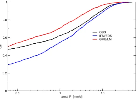
[image:5.595.51.286.63.232.2]OBS IFM/EDS GME/LM
Fig. 3. Cumulative distribution functions of Alb observations (black) and simulations (+2 d) from IFM/EDS (blue) and GME/LM (red).
scale throughout. In 2003, the difference between the fore-casts is even more striking: While IFS/EDS simulates the en-tire series quite accurately, the GME/LM misses the events almost completely. In 2004 there was an entire series of 4 strong events, and except only in one case (IFS/EDS for the third event) they were forecast quite unsatisfactory by both systems. The 2005 forecasts are similar to those of 2003. Part of the lower predictive skill of GME/LM can be traced back to the reduced variability of that system, as demonstrated by the cumulative distribution function (cdf) of the+2 d prediction of areal precipitation, shown in Fig. 3. Compared to observations, the exceedance probability of the larger scales (on the x-axis) is considerably smaller for the GME/LM, and slightly larger for the IFS/EDS.
To focus on the predictability of strong events it is con-venient to considerQ95=13.4 mm/d andQ99=27.1 mm/d,
the upper 5% and 1% quantile, respectively, of the observed areal precipitation. Table 2 shows the contingency table of the corresponding IFM/EDS and GME/LM forecasts for a lead time of+2 d, based on the validation period (1431 days). For Q95, IFM/EDS has more hits (26 vs. 6) and
fewer misses (33 vs. 53) than GME/LM, but also more false alarms (53 vs. 21). This is also reflected in the general over-prediction of IFM/EDS (79 events) and underover-prediction of GME/LM (27 events), as compared to observed 59 events. The results for Q99 are similar, although the number of
predicted events by IFM/EDS now almost equals the num-ber of observed events (16); no Q99 event is predicted by
GME/LM.
The overall quality of the binary forecasts shown in Ta-ble 2 is assessed using the Gilbert skill score (GSS, also called equitable threat score). GSS measures the hit count relative to all cases where an event was observed or focast, and scales the result in a way that random forecasts re-ceive a zero score (Wilks, 1995). ForQ95 (Q99)this gives
Table 2. Contingency table for forecasting heavy precipitation with
lead+2 d, using IFS/EDS (blue) and GME/LM (red). Upper part:
Q95, lower part:Q99.
Q95=14.6 mm EDS,LM≤Q95 EDS,LM>Q95
OBS≤Q95 1319,1351 53,21 1372
OBS>Q95 33,53 26,6 59
1352,1404 79,27
Q99=26 mm EDS,LM≤Q99 EDS,LM>Q99
OBS≤Q99 1405,1411 10,4 1415
OBS>Q99 11,16 5,0 16
1416,1427 15,4
GSS(IFS/EDS)=0.21 (0.19) and GSS(GME/LM)=0.06 (0.0), showing superior performance by IFS/EDS.
To gain more insight into the predictive power of our sys-tem, I have plotted in Fig. 4 the GSS for all lead times up to 5 days, using the usual thresholds ofQ95 andQ99along
with 0.1 mm/d (wet/dry). For all three classes the IFS/EDS forecast shows positive skill up to a lead time of+5 d. The GME/LM forecasts are worse throughout; note that Q95
forecasts improve slightly from+1 d to +2 d, which indi-cates chance behavior in view of the small GSS values; for theQ99 class there is no skill beyond a lead time of +1 d.
For comparison, I also show the performance of the persis-tence forecast, which is usually a bad predictor for precipita-tion due to its short memory; note again the chance behavior especially forQ99.
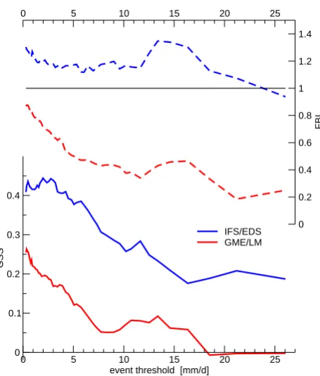
To further analyze the dependence of forecast skill on the rarity of the event Fig. 5 shows, for a lead time of+2 d, the dependence of forecast skill on the event threshold. I show both the GSS and, as a check for under- or overprediction, the frequency bias index (FBI, the ratio of the number of forecast events to the number of observed events). For both systems the GSS decreases with rarity, but throughout it is about 0.2 larger for the IFS/EDS. With respect to the FBI, the GME/LM tends towards strong underprediction with heav-ier events, as compared to fairly unbiased predictions of the IFS/EDS for all thresholds.
[image:5.595.308.548.110.223.2]0 1 2 3 4 5 lead time [d]
0 0.1 0.2 0.3 0.4
GSS
PERS IFS/EDS GME/LM wet / dry
0 1 2 3 4 5
lead time [d] 0
0.1 0.2 0.3 0.4
GSS
Q95
0 1 2 3 4 5
lead time [d] 0
0.1 0.2 0.3 0.4
GSS
[image:6.595.102.497.62.273.2]Q99
Fig. 4. For the Alb, skill (GSS) of the two forecast systems vs. lead time, using three different event classes. IFS/EDS: blue, GME/LM: red.
For comparison, persistence is used as well (gray).
0 5 10 15 20 25
event threshold [mm/d] 0
0.1 0.2 0.3 0.4
GSS
IFS/EDS GME/LM
0 5 10 15 20 25
0 0.2 0.4 0.6 0.8 1 1.2 1.4
FBI
Fig. 5. GSS and FBI dependence on event threshold (rarity), using +2 d predictions for the Alb.
Therefore, only two degrees of freedom remain: the proba-bility of a miss,PM=P (O>Q∧F≤Q), and the probability of a forecast being issued,PF=P (F >Q). With the cost of precautionary measures beingC and that of a loss incurred
from a miss beingL, the expected daily expenses amount to:
e=L·PM +C·PF. (6)
If no forecast is issued, no investment costs are generated but each occurring event is a miss. If the event probability isPE, the costs to be expected are
e0=L·PE. (7)
In general, if
PE−PM
PF
> α , (8)
whereα=C/Ldenotes the cost/loss ratio, the expected re-duction of losses outweighs the investment from the protec-tion and the forecast has positive economic effects.
For the case described in Table 2, suppose the cost for protection against a rather moderateQ95-event isC=10 k C,
and the loss isL=100 k C, thene0=0.05∗L=5 k C. Using
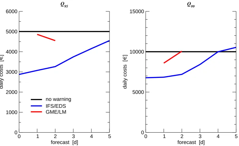
the IFS/EDS forecasts one gets a value of aboute=3.3 k C, which amounts to 1.7 k C savings per day; GME/LM fore-casts yield savings of about 500 C. This is the situation for forecasts of lead+2 d. Figure 6 displays the expected daily expenses for all lead times and both event classes. Consid-erable savings are to be expected forQ95events when using
IFS/EDS forecasts for up to lead+5 d. ForQ99events,
us-ingC=100 k C andL=1 M C, the same is true for forecasts of up to lead+3 d. Using GME/LM forecasts gives moderate savings, except for the+2 d forecast ofQ99which entails no
savings. The two examples above used a cost/loss ratio of
[image:6.595.54.282.329.597.2]0 1 2 3 4 5 forecast [d]
0 1000 2000 3000 4000 5000 6000
daily costs [
]
no warning IFS/EDS GME/LM
Q95
0 1 2 3 4 5
forecast [d] 0
5000 10000 15000
daily costs [
]
[image:7.595.104.495.62.301.2]Q99
Fig. 6. Expected daily expenses for the Alb, for aQ95 and Q99 event with no warnings (black) or warnings from IFS/EDS (blue) or
GME/LM (red).
Mar-12 Mar-17 Mar-22 Mar-27
2002 0
20 40 60
areal P [mm/d]
OBS IFS/EDS GME/LM
Sep-28 Oct-03 Oct-08 Oct-13
2003 0
20 40 60
[image:7.595.71.525.350.493.2]areal P [mm/d]
Fig. 7. Similar to Fig. 2, for the Upper Danube. (Note that observations ended in 2003).
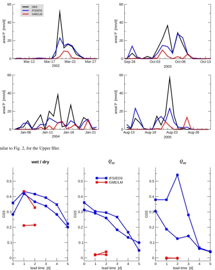
3.2 Upper Danube and Upper Iller
Despite different geographical and climatic conditions, the verification results for the Upper Danube and Upper Iller are similar to the Alb. For the Upper Danube, where data ended in 2003, the+2 d forecast of the most extreme yearly events is depicted in Fig. 7. In 2002, the most extreme event was observed on 19 March with 67 mm/d. Here the IFS/EDS forecast (32 mm/d) is only moderately better than that of GME/LM (19 mm/d). In 2003, IFS/EDS forecasts are again superior to GME/LM. Forecasts for the Upper Iller are gen-erally worse than those of the other catchments. This is ex-emplified by the yearly maxima shown in Fig. 8. Especially the 2004 and 2005 forecasts are bad for both systems. The general superiority of IFS/EDS to GME/LM is apparent from
Fig. 9. It shows that for all event classes and lead times the GSS is comparable to the skill of the Alb shown in Fig. 4. Only theQ99 skill for lead time+2 d is exceptionally high
for the Upper Danube (GSS=0.54). It is unknown whether this is a random effect (data ended in 2003) or indicative of a real feature.
4 Discussion
Mar-12 Mar-17 Mar-22 Mar-27 2002
0 20 40 60
areal P [mm/d]
OBS IFS/EDS GME/LM
Sep-28 Oct-03 Oct-08 Oct-13
2003 0
20 40 60
areal P [mm/d]
Jan-06 Jan-11 Jan-16 Jan-21
2004 0
20 40 60
areal P [mm/d]
Aug-13 Aug-18 Aug-23 Aug-28
2005 0
20 40 60
[image:8.595.83.515.59.602.2]areal P [mm/d]
Fig. 8. Similar to Fig. 2, for the Upper Iller.
0 1 2 3 4 5
lead time [d] 0
0.1 0.2 0.3 0.4 0.5
GSS
IFS/EDS GME/LM wet / dry
0 1 2 3 4 5
lead time [d] 0
0.1 0.2 0.3 0.4 0.5
GSS
Q95
0 1 2 3 4 5
lead time [d] 0
0.1 0.2 0.3 0.4 0.5
GSS
Q99
Fig. 9. Similar to Fig. 4, the GSS for the other two catchments. Upper Danube (square) and Upper Iller (circle).
to at least 3, maybe 5 days in advance. For all event classes and lead times that system outperformed the GME/LM sys-tem. The crucial question is now which of the components makes the difference. But since the systems are so deeply intermingled one feels that deciding that question is hard if
Whatever the reported differences in skill are, they appear marginal in relation to those of, e.g., Fig. 2 or Fig. 5. These +2 d forecasts reveal a gap in skill that can hardly be as-cribed to the driving models. This is further supported by the GME/LM failure to reproduce local variability, as evidenced by Fig. 3 and compared to the fairly unbiased local variability of the GME at least in its 2008-version. Therefore, I would ascribe the observed skill differences mainly to the down-scaling. It is not unlikely that what we see here is related to the well known luv-lee problem of many high-resolution dynamic models (Baldauf and Schulz, 2004; Elementi et al., 2005), where in mountainous terrain too much rainfall is pro-duced on the luv side and too little on the lee side.
The luv-lee problem illuminates the differences between dynamical and empirical downscaling models mentioned in the introduction: Being genuinely three-dimensional the dy-namical models simulate high-resolution precipitation for an entire domain. But the parameterizations of the unresolved scales – here: the advection of falling rain – introduce imper-fections that over complex terrain can have a large impact on the water balance. Empirical models, on the other hand, have “seen” the luv–lee characteristic during calibration and “re-member” it when confronted with a particular weather type. But a large-scale/small-scale relation like this may as well be more complicated, nonlinear for example, which would then require a revision of the transfer function class and a re-fitting with extra parameters. One should note, however, that if this revision comes after the fact independent validation with the same data is no longer possible. Some a priori physical in-sight is therefore desirable even for empirical models.
A major drawback in the current setup of the IFS/EDS is the determination of the number of EOFs to be retained. Here it was done by simply cross-checking some validation statistics for various lead times, and selecting a number that appeared optimal on average. For Alb, Upper Danube, and Upper Iller this was 81, 79, and 114 EOFs, respectively. Due to data limitations this was done using the entire dataset, so the verification statistics shown above are not fully indepen-dent. However, dependence on the number of EOFs was in general fairly weak over a broad range of values, so that the main results are not affected by this choice. This step should nevertheless be improved in future work, for example, by us-ing more elaborate cross validation techniques.
It should be noted that probabilistic versions of the IFS/EDS system exist and have also been applied to the three catchments (cf. OPAQUE, http://brandenburg.geoecology. uni-potsdam.de/projekte/opaque). This was done simply by replacing the deterministic IFS forecast by the ensemble pre-diction system of the ECMWF (B¨urger et al., 2009). In these applications, the use of probabilistic information indeed im-proves the forecasts, especially for the longer lead times be-yond+3 d.
Acknowledgements. This study was conducted as part of the project OPAQUE which was funded by the Federal Ministry of Ed-ucation and Research, Germany. I am grateful to the Landesanstalt f¨ur Umwelt, Messungen und Naturschutz Baden-W¨urttemberg who kindly provided the LM forecast data.
Edited by: A. Gelfan
References
B¨urger, G.: Expanded downscaling for generating local weather scenarios, Clim. Res., 7, 111–128, 1996.
B¨urger, G.: Selected precipitation scenarios across Europe, J. Hy-drol., 262(1–4), 99–110, 2002.
B¨urger, G., Fast, I., and Cubasch, U.: Climate reconstruction by regression-32 variations on a theme, Tellus A, 58(1), 227–235, 2006.
B¨urger, G., Reusser, D., and Kneis, D.: Early flood warnings from empirical (expanded) downscaling of the full Ensemble Predic-tion System, Water Resour. Res., doi:10.1029/2009WR007779, in press, 2009.
Baldauf, M. and Schulz, J. P.: Prognostic precipitation in the Lokal-Modell (LM) of DWD, COSMO Newsletter, 4, 177–180, 2004. Bartholmes, J. C., Thielen, J., Ramos, M. H., and Gentilini, S.: The
european flood alert system EFAS – Part 2: Statistical skill as-sessment of probabilistic and deterministic operational forecasts, Hydrol. Earth Syst. Sci., 13, 141–153, 2009,
http://www.hydrol-earth-syst-sci.net/13/141/2009/.
Charba, J. P., Reynolds, D. W., McDonald, B. E., and Carter, G. M.: Comparative verification of recent quantitative precipitation forecasts in the National Weather Service: A simple approach for scoring forecast accuracy, Weather Forecast., 18(2), 161–183, 2003.
Clark, M. P. and Hay, L. E.: Use of medium-range numerical weather prediction model output to produce forecasts of stream-flow, J. Hydrometeorol., 5(1), 15–32, 2004.
Damrath, U., Doms, G., Fr¨uhwald, D., Heise, E., Richter, B., and Steppeler, J.: Operational quantitative precipitation forecasting at the German Weather Service, J. Hydrol., 239(1–4), 260–285, 2000.
Ebert, E. E., Damrath, U., Wergen, W., and Baldwin, M. E.: The WGNE assessment of short-term quantitative precipitation fore-casts, Bull. Am. Meteorol. Soc., 84(4), 481–492, 2003. Elementi, M., Marsigli, C., and Paccagnella, T.: High resolution
forecast of heavy precipitation with Lokal Modell: analysis of two case studies in the Alpine area, Nat. Hazards Earth Syst. Sci., 5, 593–602, 2005,
http://www.nat-hazards-earth-syst-sci.net/5/593/2005/.
Hamill, T. M., Whitaker, J. S., and Mullen, S. L.: Reforecasts: An Important Dataset for Improving Weather Predictions, Bull. Am. Meteorol. Soc., 87(1), 33–46, 2006.
Ledermann, W., Churchhouse, R. F., and Vajda, S.: Handbook of Applicable Mathematics: Statistics, John Wiley & Sons, 1984. Liu, X., Coulibaly, P., and Evora, N.: Comparison of data-driven
methods for downscaling ensemble weather forecasts, Hydrol. Earth Syst. Sci., 12, 615–624, 2008,
http://www.hydrol-earth-syst-sci.net/12/615/2008/.
op-erational global icosahedral–hexagonal gridpoint model GME: Description and high-resolution tests, Month. Weath. Rev., 130(2), 319–338, 2002.
McBride, J. L. and Ebert, E. E.: Verification of quantitative precip-itation forecasts from operational numerical weather prediction models over Australia, Weather Forecast., 15(1), 103–121, 2000. Menzel, L., Thieken, A. H., Schwandt, D., and B¨urger, G.: Impact of climate change on the regional hydrology – scenario-based modelling studies in the German Rhine catchment, Nat. Haz., 38(1), 45–61, 2006.
Richard, E., Buzzi, A., and Zangl, G.: Quantitative precipitation forecasting in the Alps: The advances achieved by the Mesoscale Alpine Programme, Q. J. R. Meteorol. Soc., 133(625), 831–846, 2007.
Thompson, J. C.: On the operational deficiencies in categorical weather forecasts, Bull. Amer. Meteor. Soc, 33, 223–226, 1952. White, B. G., Paegle, J., Steenburgh, W. J., Horel, J. D.,
Swan-son, R. T., Cook, L. K., Onton, D. J., and Miles, J. G.: Short-term forecast validation of six models, Weather Forecast., 14(1), 84–108, 1999.
White, P. W.: IFS Documentation, ECMWF, Reading, 2002. Wilks, D. S.: Statistical methods in the atmospheric sciences,