A comparative analysis of two wind velocity retrieval techniques by using a single Doppler radar

(1)

Hydrol. Earth Syst. Sci., 13, 651–661, 2009 www.hydrol-earth-syst-sci.net/13/651/2009/ © Author(s) 2009. This work is distributed under the Creative Commons Attribution 3.0 License.

Hydrology and

Earth System

Sciences

A comparative analysis of two wind velocity retrieval techniques by

using a single Doppler radar

H.-C. Lim1and D.-I. Lee2

1_{School of Mechanical Engineering, PuKyong National University, San 100, Yongdang-Dong, Nam-Gu, Busan, 608-739,}

South Korea

2_{Department of Environment and Atmospheric Science, PuKyong National University, 599-1, Daeyon-Dong, Nam-Gu,}

Busan, 608-737, South Korea

Received: 18 January 2009 – Published in Hydrol. Earth Syst. Sci. Discuss.: 24 February 2009 Revised: 16 May 2009 – Accepted: 19 May 2009 – Published: 26 May 2009

Abstract. This study compares the theoretical basis of the

two wind velocity retrieval methods, Velocity Azimuth Dis-play (VAD) and Velocity Area DisDis-play (VARD) by using data obtained by a single Doppler radar. Two pre-assumed shapes of the wind velocity distribution with altitude are considered, uniform and parabolic. The former presents an approxima-tion of the non-sheared or low-sheared wind flow in the up-per troposphere, while the latter is a simplified representation of the Atmospheric Boundary Layer (ABL) in lower sphere or high-sheared wind flow at the edges of the tropo-spheric jet streams. Both techniques for the wind velocity retrieval considered in this study are reformulated in order to get more precise information on the wind velocity compo-nents. An algorithm is proposed to decrease the uncertainty in retrieving by evaluating the coefficients of the polynomial equation and applying a transfer function with respect to the angle formed between the wind flow direction and direction of radar beam. It is concluded that, provided the formu-lated transformation functions are used, the application of the VAD and VARD techniques to the single-Doppler data may be an invaluable tool for solving various climate and wind engineering problems.

Correspondence to: D.-I. Lee ([email protected])

1 Introduction

Changes in climate have had an increasing impact on wind environment of the Korean peninsula over the last decade. For example, several deadly typhoons such as Funsen and Rusa struck the Korean coast in 2002, while the typhoon Ewiniar, the 3rd largest in 2006, was particularly dread-ful causing a great damage in a short period. Therefore, the importance of forecasting wind velocity features and maintaining an appropriate level of readiness and prepared-ness for similar disasters is beyond question. The forecast of wind parameters such as its speed, direction or conver-gence/divergence features, however, still remains a main con-cern of the meteorological services and the observatories.

(2)

652 H.-C. Lim and D.-I. Lee: Wind velocity retrieval techniques by a Doppler radar 8 H.-C. LIM & D.-I. LEE: Wind Velocity Retrieval Techniques by a Doppler Radar

V

Radar sweep

V

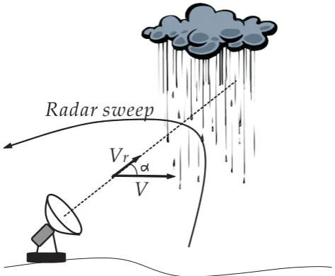
r

Fig. 1. A sketch showing the relationship between the radial

ve-locity of the moving target, Vr, and real target velocity,V. Only the radial target velocity may be retrieved be a single Doppler radar without any additional assumptions. The angleαis formed between the direction in which the radar beam is pointed and direction in which target moves.

V

x

V

r

θ

Ф

y

Ф

R

Rsin

z

Fig. 2. Geometry of radar scan from Browning and Wexler (1968)

4x/D

-2

0

2

4y/D

-2 -1

0 1

2

4z

/D

0 1 2

4x/D -2

0

2

4y/D

-2 -1

0 1

2

4z

/D

0 1 2

Fig. 3. Virtual domain for generating the wind profiles (a) in the

rec-tangular coordinate (upper) (b) in the spherical coordinate (lower)

ve-locity of the moving target,Vr, and real target velocity,V. Only

the radial target velocity may be retrieved be a single Doppler radar without any additional assumptions. The angleαis formed between the direction in which the radar beam is pointed and direction in which target moves.

As described below, a number of radar studies have been carried out to obtain an appropriate three-dimensional dis-tribution of the extreme wind fields in typhoons and heavy rainfall during summer monsoon season. Many developed countries spent a lot of time in trying to make an accurate re-trieval of wind velocity fields from radars; whereas the stud-ies on these retrieval methods in Korea were relatively out of primary concern. Lack of high performance radar, trained human resources and appropriate funding may be few rea-sons for relatively rare appearance of such kind of studies in Korea.

The antenna of the radar usually rotates around a vertical axis, scanning the horizon in all directions. Figure 1 shows the geometric relationship between the directions which a target (cloud or rain drops) moves and the direction in which antenna is pointed. A challenge is here to obtain information concerning the total target velocity, which may be carried out only with certain additional suppositions.

Lhermitte and Atlas (1961) were the first to demonstrate the crucial importance of the magnitude and direction of the mean horizontal wind velocity retrieved from radial veloc-ity data. The proposed technique using the data processed from horizontal concentric circles centered at the radar site was called Velocity Azimuth Display (VAD). Caton (1963) and Browning and Wexler (1968) demonstrated that simi-lar concept may be extended to yield other important pa-rameters such as mean convergence, stretching and shear-ing deformation. They assumed that the wind vector field varies linearly in the horizontal plane. When using the VAD

technique, it is not possible to separate the contributions of the vertical wind velocity and the hydrometer fall velocity to the total vertical velocity. Moreover, an additional prob-lem is the divergence of the horizontal wind field. Improved versions of the VAD technique designed to properly sepa-rate various contributions were developed in the late eighties and early nineties and have been dubbed the extended-VAD (EVAD) technique (Srivastava et al., 1986) and the concur-rent extended-VAD(CEVAD) technique (Matejka, 1993). In-stead of processing a single VAD or a series of VADs, one can only process the low altitudes (φ≈0, z0≈0) which are of

greater interest than the other data. This method called Ve-locity ARea Display(VARD) was developed by Easterbrook (1975). His study was dealing with processing data in a con-ical sector rather than along a circle. Easterbrook showed that five parameters of the wind field may be extracted from such data; however, unless additional information is avail-able, the mean horizontal velocity is contaminated by vortic-ity and cannot be completely determined. Nowadays, both the VAD and VARD techniques, as well as newly developed tools such as EVAD or Volume Velocity Processing (VVP) are widely used to retrieve wind profiles from Doppler radar observations.

Despite the widespread use of the VAD and VARD re-trieval techniques, only a few verification or case studies involving the retrieved wind profiles have been reported so far. Moreover, evaluations between the VAD and VARD re-trieval techniques applied to horizontal wind velocity data have been rarely published up to now. For example, Ander-son (1998) published the results of verification study compar-ing VAD wind profiles with those obtained by uscompar-ing either radiosonde or numerical weather prediction involving the High Resolution Limited Area Model (HIRLAM). The ac-tual wind in the atmosphere is fairly complicated, frequently changing significantly from one level to the next. Moreover, the magnitude of wind may changes over time and space. To describe such velocity fields accurately, the best approach is to make a simultaneous measurement by three Doppler radars. However, such measurement systems are fairly ex-pensive and cover very limited area and thus rarely been ac-complished. Most of the studies up to now were carried out by using reduced instrumental system involving two or one Doppler radar. We carry out some further analysis along this line and study the generalization of the wind field by process-ing the data from sprocess-ingle-Doppler radar in volume, assumprocess-ing linearity of the wind field distribution. The emphasis in this study is placed on a radar system for retrieval of wind veloc-ity fields over Korea. In addition, we present some compar-ison of different implementation of the VAD and VARD re-trieval techniques by using two shapes of the reference wind profiles, uniform and parabolic.

[image:2.595.49.286.63.258.2]

(3)

H.-C. Lim and D.-I. Lee: Wind velocity retrieval techniques by a Doppler radar 653 8 H.-C. LIM & D.-I. LEE: Wind Velocity Retrieval Techniques by a Doppler Radar

V

Radar sweep

V

r

ve-locity of the moving target,Vr, and real target velocity, V. Only the radial target velocity may be retrieved be a single Doppler radar without any additional assumptions. The angleαis formed between the direction in which the radar beam is pointed and direction in which target moves.

V

x

V

r

θ

Ф

y

Ф

R

Rsin

z

Fig. 2. Geometry of radar scan from Browning and Wexler (1968)

4x/D

-2

0

2

4y/D

-2 -1

0 1

2

4z

/D

0 1 2

4x/D -2

0

2

4y/D

-2 -1

0 1

2

4z

/D

0 1 2

Fig. 3. Virtual domain for generating the wind profiles (a) in the

rec-tangular coordinate (upper) (b) in the spherical coordinate (lower)

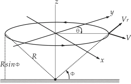
Fig. 2. Geometry of radar scan from Browning and Wexler (1968).

2 Analysis of the mean wind field

2.1 Processing the velocity field

As stated above, the success of the VAD and VARD tech-niques in predicting three-dimensional wind field heavily de-pends on the value of the angle formed between direction in which wind is blowing and direction in which antenna is pointed. Therefore, to analyze the role of all factors involved in application of those techniques, we reformulated those methods, i.e. VAD, VARD (Waldteufel and Corbin, 1978).

Consider a Cartesian coordinate system (x, y, z) (see Fig. 2), whose origin 0 is at the radar, with vertical axisz

directed upward and axesxandydirected to the east and the north, respectively. The spherical coordinatesR,φ, andθof the measured point are associated with the Cartesian system, whereRis the range,φis the elevation angle, andθis the az-imuth angle starting from the north. Assume that the velocity vector of the motion of scattersV=(u, v, w) varies linearly around its value (u0, v0, w0) at a point (x0, y0, z0) and may

be represented as follows:

u=u0+du_dx(x−x0)+_dydu(y−y0)+du_dz(z−z0)

v =v0+dv_dx(x−x0)+_dydv(y−y0)+dv_dz(z−z0)

w=w0+dw_dx(x−x0)+dw_dy(y−y0)+dw_dz(z−z0)

(1)

Then the radial velocityVr measured by the radar may be written as follows,

Vr = −ucosθcosφ−vsinθcosφ−wsinφ (2)

whereθandφare the azimuth and elevation angles. Trans-forming from rectangular to polar coordinates, introducing

the radial distance R and regrouping terms, the following equation may be obtained

Vr ≈cosθcosφu0+sinθcosφv0+sinφw0

+Rcos2θcos2φ (du/dx)+Rsin2θcos2φ (dv/dy) +Rsinθcosφcos2φ (du/dy+dv/dx)

+sinφ (Rsinφ−z0)dw/dz

+cosθcosφ (Rsinφ−z0)du/dz

+sinθcosφ (Rsinφ−z0)dv/dz

(3)

In Eq. (3), only terms with different azimuth dependence can be discriminated. SinceR andφare constant, we can regroup terms in Eq. (3) to obtain equation used in the VAD method.

Vr ≈cosθcosφu0+sinθcosφv0

+cos2θ[Rcos2φ (du/dx)+sinφw0]

+sin2θ[Rcos2φ (dv/dy)+sinφw0]

+sinθcosθ Rcos2(du/dy+dv/dx)

(4)

The VARD method proposed by Easterbrook (1975), is also applied for a conical sector, i.e., x06=0,y06=0.

There-fore, when low elevation angles are considered (sinφ∼0, cosφ∼1), the Eq. (3) becomes

Vr ≈cosθ (u0−x0du/dx−y0du/dy)

+Rsinθ (v0−x0dv/dx−y0dv/dy)

+Rcos2θ du/dx+Rsin2θ dv/dy +Rcosθsinθ (du/dy+dv/dx)

(5)

In Eq. (5), there are only terms regarding the horizontal plane so that it appears to be a two-dimensional linear equa-tion. Given that the reference wind fields are provided, all derivatives as well as the trigonometric functions can be eas-ily retrieved. Note here that the vorticity and mean horizontal wind components are combined in the first two terms and the differential properties of the horizontal wind field would be known to be restricted to low elevation angle (lower than 5◦_), as Easterbrook proposed. Therefore, the current calculation can confirm the vertical/horizontal velocity component vary-ing with altitude even though the equation is restricted to low elevations.

2.1.1 Reference wind field in a virtual pseudo-domain

[image:3.595.52.283.66.215.2]

(4)

654 H.-C. Lim and D.-I. Lee: Wind velocity retrieval techniques by a Doppler radar

8 H.-C. LIM & D.-I. LEE: Wind Velocity Retrieval Techniques by a Doppler Radar

V

Radar sweep

V

r

Fig. 1. A sketch showing the relationship between the radial

ve-locity of the moving target,

V

_r

, and real target velocity,

V

. Only

the radial target velocity may be retrieved be a single Doppler radar

without any additional assumptions. The angle

α

is formed between

the direction in which the radar beam is pointed and direction in

which target moves.

V

x

V

r

θ

Ф

y

Ф

R

Rsin

z

Fig. 2. Geometry of radar scan from Browning and Wexler (1968)

4x/D

-2

0

2

4y/D

-2 -1

0 1

2

4z

/D

0 1 2

4x/D

-2

0

2

4y/D

-2 -1

0 1

2

4z

/D

0 1 2

Fig. 3. Virtual domain for generating the wind profiles (a) in the

rec-tangular coordinate (upper) (b) in the spherical coordinate (lower)

8 H.-C. LIM & D.-I. LEE: Wind Velocity Retrieval Techniques by a Doppler Radar

V

Radar sweep

V

r

Fig. 1. A sketch showing the relationship between the radial

ve-locity of the moving target,

V

_r

, and real target velocity,

V

. Only

the radial target velocity may be retrieved be a single Doppler radar

without any additional assumptions. The angle

α

is formed between

the direction in which the radar beam is pointed and direction in

which target moves.

V

x

V

r

θ

Ф

y

Ф

R

Rsin

z

Fig. 2. Geometry of radar scan from Browning and Wexler (1968)

4x/D

-2

0

2

4y/D

-2 -1

0

1 2

4z

/D

0 1 2

4x/D

-2

0

2

4y/D

-2

-1 0

1 2

4z

/D

0 1 2

Fig. 3. Virtual domain for generating the wind profiles (a) in the

rec-tangular coordinate (upper) (b) in the spherical coordinate (lower)

Fig. 3. Virtual domain for generating the wind profiles (a) in

the rectangular coordinate (upper) (b) in the spherical coordinate (lower).

Figure 3 compares the size and shape of the vir-tual pseudo-domains obtained in Cartesian and spheri-cal coordinate system. The size of the Cartesian co-ordinate system is 2width×2length×1height non-dimensional units (i.e. 4x/D, 4y/D and 4z/D) and the numbers of grid are 50×50×25. The size of the spherical sys-tem is 2 non-dimensional units, and the number of grid points are 30radial×30azimuth×30elevation. Each axis is non-dimensionalized byD/4, which is, in fact, the representative length of the pseudo-domain.

Figure 4 shows the reference wind velocity profiles allo-cated in the virtual domain. The case of the uniform wind flow (dashed line) with a constant velocity(e.g.∼1) through-out the scanned layer is unrealistic, however, it is easy to deal with it. The parabolic or power-law profile (solid line) mod-els the boundary layer with effect of surface roughness and, therefore, is closer to the real situation in the atmosphere. Comparing these two profiles, it is possible to analyze the ef-fect of the atmospheric boundary layer on the air flow near to the ground. We refer to these particular velocity patterns as “wind signatures” according to the research by Armstrong and Donaldson (1969) and Wood and Brown (1986, 1997). Armstrong and Donaldson considered a series of

concen-H.-C. LIM & D.-I. LEE: Wind Velocity Retrieval Techniques by a Doppler Radar 9

0 0.5 1 1.5 2

0 0.5 1 1.5

U

z

Uniform parabolic

Fig. 4. Distributions of the streamwise wind velocity component,

U, retrieved by using VAD method and two shapes of the reference wind velocity distribution: uniform (on the left-hand side) and par-abolic (on the right-hand side).

4x/D -2

-1 0

1 2

4y/D

-2 -1

0 1

2

4z

/D

0 0.5 1 1.5 2

U:00.1 0.2 0.3 0.4 0.5 0.6 0.7 0.8 0.91

4x/D

-2 -1 0 1 2

4y/D

-2 -1 0 1 2

4z/

D

0 0.5 1 1.5 2

U, retrieved by using VAD method and two shapes of the reference wind velocity distribution: uniform (on the left-hand side) and par-abolic (on the right-hand side).

4x/D -2 -1

0 1

2

4y/D

-2 -1

0 1

2

4z

/D

0 0.5 1 1.5 2

U:00.1 0.2 0.3 0.4 0.5 0.6 0.7 0.8 0.91

4x/D

-2 -1 0 1 2

4y/D

-2 -1 0 1 2

4z/

D

0 0.5 1 1.5 2

Fig. 6. The same as in Fig. 5, but using VARD method.

4x/D -2 -1

0

1 2

4y/D

-2 -1

0 1

2

4z

/D

0 0.5 1 1.5 2

W:-1 -0.8 -0.6 -0.4 -0.2 00.2 0.4 0.6 0.81

4x/D

-2 -1 0 1 2

4y/D

-2 -1 0 1 2

4z/

D

0 0.5 1 1.5 2

Fig. 7. Distributions of the vertical wind velocity component,W,

retrieved by using VAD method and two shapes of the reference wind velocity distributions: uniform (on the left-hand side) and par-abolic (on the right-hand side).

4x/D -2

-1 0

1 2

4y/D

-2 -1

0 1

2

4z

/D

0 0.5 1 1.5 2

W:-1 -0.8 -0.6 -0.4 -0.2 00.2 0.4 0.6 0.81

4x/D

-2 -1 0 1 2

4y/D

-2 -1 0 1 2

4z/

D

0 0.5 1 1.5 2

4x/D

-2 -1 0 1 2

4y/D

-2 -1

0 1

2

4z/

D

0 1 2

PARABOLIC /VAD PARABOLIC

/VARD

(b) Parabolic reference wind

4x/D

-2 -1 0 1 2

4y/D

-2 -1

0 1

2

4z/

D

0 1 2

U: 00.1 0.2 0.3 0.4 0.5 0.6 0.7 0.8 0.91

UNIFORM /VAD UNIFORM

/VARD

(a) Uniform reference wind

Fig. 9. Combined contour plots of the streamwise wind velocity component,U, on the surface of calculated domain varying as func-tions of elevation and azimuth for two reference wind velocity dis-tributions: (a) uniform ; (b) parabolic. The calculated domain in both cases is divided into two halves showing the results obtained by applying VARD and VAD techniques, on the left-hand half and on the right-hand half, respectively.

U, retrieved by using VAD method and two shapes of the refer-ence wind velocity distribution: uniform (on the left-hand side) and parabolic (on the right-hand side).

tric arcs produced at a Plan Shear Indicator (PSI) display. This procedure allowed them to identify a small scale vor-tex, such as a meso-cyclone or tornado, from the observed tangential shear of the radial velocity. Wood and Brown pro-duced computer-simulated pictures for various pre-assumed non-divergent wind velocity distributions. They used as a pattern the isopleths of constant Doppler velocity which they called isodops.

The typical procedure to retrieve the wind flow field in-cludes: (i) generation of the virtual domain and allocation of the input environmental velocity; (ii) retrieval of the radial velocity by using VAD/VARD transformation; (iii) compar-ison of the real and the transformed velocities. More detail procedure will be explained in due course.

3 Results and discussion

Firstly, we present the calculated three-dimensional (3-D) distributions of the retrieved wind velocity components ob-tained by using both VAD and VARD techniques and by ap-plication of two proposed shapes of the reference wind ve-locity profiles. Then, a detailed analysis will be given of the calculated results. Finally, by using the mathematical tech-niques described below, it is possible to improve the applica-tion of the retrieved informaapplica-tion from the Doppler radar and to get the shapes of retrieved wind velocity profiles closer to the pre-assumed shapes.

(5)

H.-C. Lim and D.-I. Lee: Wind velocity retrieval techniques by a Doppler radar 655

H.-C. LIM & D.-I. LEE: Wind Velocity Retrieval Techniques by a Doppler Radar 9

0 0.5 1 1.5 2

0 0.5 1 1.5

U

z

Uniform parabolic

Fig. 4. Distributions of the streamwise wind velocity component, U, retrieved by using VAD method and two shapes of the reference wind velocity distribution: uniform (on the left-hand side) and par-abolic (on the right-hand side).

4x/D -2 -1 0 1 2 4y/D -2 -1 0 1 2 4z /D 0 0.5 1 1.5 2

U:00.1 0.2 0.3 0.4 0.5 0.6 0.7 0.8 0.91

4x/D -2 -1 0 1 2 4y/D -2 -1 0 1 2 4z/ D 0 0.5 1 1.5 2

4x/D -2 -1 0 1 2 4y/D -2 -1 0 1 2 4z /D 0 0.5 1 1.5 2

U:00.1 0.2 0.3 0.4 0.5 0.6 0.7 0.8 0.91

4x/D -2 -1 0 1 2 4y/D -2 -1 0 1 2 4z/ D 0 0.5 1 1.5 2

4x/D -2 -1 0 1 2 4y/D -2 -1 0 1 2 4z /D 0 0.5 1 1.5 2

W:-1 -0.8 -0.6 -0.4 -0.2 00.2 0.4 0.6 0.81

4x/D -2 -1 0 1 2 4y/D -2 -1 0 1 2 4z/ D 0 0.5 1 1.5 2

4x/D -2 -1 0 1 2 4y/D -2 -1 0 1 2 4z /D 0 0.5 1 1.5 2

W:-1 -0.8 -0.6 -0.4 -0.2 00.2 0.4 0.6 0.81

4x/D -2 -1 0 1 2 4y/D -2 -1 0 1 2 4z/ D 0 0.5 1 1.5 2

4x/D -2 -1 0 1 2 4y/D -2 -1 0 1 2 4z/ D 0 1 2 PARABOLIC /VAD PARABOLIC /VARD

4x/D -2 -1 0 1 2 4y/D -2 -1 0 1 2 4z/ D 0 1 2

U: 0 0.1 0.2 0.3 0.4 0.5 0.6 0.7 0.8 0.9 1

/VARD

Fig. 9. Combined contour plots of the streamwise wind velocity

component,U, on the surface of calculated domain varying as func-tions of elevation and azimuth for two reference wind velocity dis-tributions: (a) uniform ; (b) parabolic. The calculated domain in both cases is divided into two halves showing the results obtained by applying VARD and VAD techniques, on the left-hand half and on the right-hand half, respectively.

U, retrieved by using VAD method and two shapes of the refer-ence wind velocity distribution: uniform (on the left-hand side) and parabolic (on the right-hand side).

3.1 Analysis of the overall flow around the radar site

In reality, the antenna of a scanning Doppler radar makes a rotation of 360◦ _{per several seconds at a specific} tion, and then the scanning is continued at a new eleva-tion. This procedure continues until the entire volume around the radar is scanned. The information on the scanned vol-ume is obtained by superposition of the information from the radar beams at different elevation angles. For the sake of simplicity, the shape of beams is considered to be con-ical, while each of them may be divided into equi-spaced volumes containing information on the reflectivity of the tar-get and the radial component of the wind velocity in the scanned volume. If the approximate shape of the wind veloc-ity distribution with altitude in the environment is given, then both the streamwise and vertical components of the wind velocity may be derived. However, depending on the pre-assumed shape of the wind velocity profile, completely dif-ferent results may be retrieved. In Fig. 5, the two calcula-tion results are compared of the streamwise velocity com-ponent, both of them obtained by using the VAD method, but with different pre-assumed wind velocity distributions with altitude: uniform, U=(U,0,0), on the left-hand side, and parabolic, U=(az2,0,0), on the right-hand side. The retrieved velocities are divided by the maximal value of pre-assumed velocity to obtain a non-dimensionalized field rang-ing from 0 to 1. The contours of approximately equal val-ues of non-dimensional velocity are drawn at every 0.1 unit, while the black-grey scale is used to distinguish the lower values (black) from the higher values (grey) of the non-dimensional velocity. Thus, the grey-contoured fields des-ignate the calculation domains where the retrieved values match pre-assumed ones perfectly, while the black-contoured fields designate the domains with poor coincidence. To clearly visualize the domains with different degree of match-ing inside the calculated volumes, the figure presents the cross-section of the calculated wind velocity fields. One may conclude from Fig. 5 that the degree of matching between the retrieved wind velocity fields and the pre-assumed ones is completely different in the case of uniform and parabolic pre-assumed wind velocity distributions. In the former case

0 0.5 1 1.5 2

0 0.5 1 1.5

U

z

Uniform parabolic

4x/D -2 -1 0 1 2 4y/D -2 -1 0 1 2 4z /D 0 0.5 1 1.5 2

U:00.1 0.2 0.3 0.4 0.5 0.6 0.7 0.8 0.91

4x/D -2 -1 0 1 2 4y/D -2 -1 0 1 2 4z/ D 0 0.5 1 1.5 2

4x/D -2 -1 0 1 2 4y/D -2 -1 0 1 2 4z /D 0 0.5 1 1.5 2

U:00.1 0.2 0.3 0.4 0.5 0.6 0.7 0.8 0.91

4x/D -2 -1 0 1 2 4y/D -2 -1 0 1 2 4z/ D 0 0.5 1 1.5 2

4x/D -2 -1 0 1 2 4y/D -2 -1 0 1 2 4z /D 0 0.5 1 1.5 2

W:-1 -0.8 -0.6 -0.4 -0.2 00.2 0.4 0.6 0.81

4x/D -2 -1 0 1 2 4y/D -2 -1 0 1 2 4z/ D 0 0.5 1 1.5 2

4x/D -2 -1 0 1 2 4y/D -2 -1 0 1 2 4z /D 0 0.5 1 1.5 2

W:-1 -0.8 -0.6 -0.4 -0.2 00.2 0.4 0.6 0.81

4x/D -2 -1 0 1 2 4y/D -2 -1 0 1 2 4z/ D 0 0.5 1 1.5 2

4x/D -2 -1 0 1 2 4y/D -2 -1 0 1 2 4z/ D 0 1 2

U: 0 0.1 0.2 0.3 0.4 0.5 0.6 0.7 0.8 0.9 1

/VARD

the best agreement is obtained near to the ground at low ele-vations when the radar is pointed in the directions either up-stream or downup-stream to the blowing wind, i.e., westward or eastward, while in the latter case the agreement is observed in the same directions but at some height above the ground. Such result has been normally anticipated considering that the angle formed between the directions of the radar beam and blowing wind is minimal in such cases. As the elevation increases and/or azimuth changes from these two unique di-rections, the above mentioned angle increases and the possi-bility for correct evaluation of the real velocity drastically de-clines. When the radar is pointed vertically up or in the direc-tion normal to the blowing wind, i.e. northward or southward, the retrieving of the wind velocity data is theoretically and practically impossible. In the case of a parabolic wind veloc-ity distribution, the function of the non-dimensional retrieved wind velocity possesses well-expressed minimum near to the ground at all azimuths. This is only a consequence of the proposed way of non-dimensionalization. Since the pre-assumed velocity decreases significantly as one approaches to the ground, the division by maximum wind velocity pro-duces misleading minimum near to the ground. As a re-sult, the two cone-shaped zones of maximum of the non-dimensional wind velocity are placed at some height above the ground in the directions upstream and downstream to the blowing wind, i.e., westward and eastward. The heights at which these maximums can be observed depend, in such a formulation, on the shape of parabolic pre-assumed wind ve-locity distribution.

Figure 6 presents the calculation results of the streamwise velocity component obtained by using the VARD technique for the same two pre-assumed wind velocity distributions with altitude. No significant difference is observed between Figs. 5 and 6 except that the uncertainty domain observed above the radar site when it is pointed vertically is signifi-cantly narrower in the case of application of VARD method as compared to the VAD method.

(6)

0 0.5 1 1.5 2

0 0.5 1 1.5

U

z

Uniform parabolic

4x/D -2 -1 0 1 2 4y/D -2 -1 0 1 2 4z /D 0 0.5 1 1.5 2

U:00.1 0.2 0.3 0.4 0.5 0.6 0.7 0.8 0.91

4x/D -2 -1 0 1 2 4y/D -2 -1 0 1 2 4z/ D 0 0.5 1 1.5 2

4x/D -2 -1 0 1 2 4y/D -2 -1 0 1 2 4z /D 0 0.5 1 1.5 2

U:00.1 0.2 0.3 0.4 0.5 0.6 0.7 0.8 0.91

4x/D -2 -1 0 1 2 4y/D -2 -1 0 1 2 4z/ D 0 0.5 1 1.5 2

4x/D -2 -1 0 1 2 4y/D -2 -1 0 1 2 4z /D 0 0.5 1 1.5 2

W:-1 -0.8 -0.6 -0.4 -0.2 00.2 0.4 0.6 0.81

4x/D -2 -1 0 1 2 4y/D -2 -1 0 1 2 4z/ D 0 0.5 1 1.5 2

4x/D -2 -1 0 1 2 4y/D -2 -1 0 1 2 4z /D 0 0.5 1 1.5 2

W:-1 -0.8 -0.6 -0.4 -0.2 00.2 0.4 0.6 0.81

4x/D -2 -1 0 1 2 4y/D -2 -1 0 1 2 4z/ D 0 0.5 1 1.5 2

4x/D -2 -1 0 1 2 4y/D -2 -1 0 1 2 4z/ D 0 1 2

U: 0 0.1 0.2 0.3 0.4 0.5 0.6 0.7 0.8 0.9 1

/VARD

retrieved by using VAD method and two shapes of the reference wind velocity distributions: uniform (on the left-hand side) and parabolic (on the right-hand side).

0 0.5 1 1.5 2

0 0.5 1 1.5

U

z

Uniform parabolic

4x/D -2 -1 0 1 2 4y/D -2 -1 0 1 2 4z /D 0 0.5 1 1.5 2

U:00.1 0.2 0.3 0.4 0.5 0.6 0.7 0.8 0.91

4x/D -2 -1 0 1 2 4y/D -2 -1 0 1 2 4z/ D 0 0.5 1 1.5 2

4x/D -2 -1 0 1 2 4y/D -2 -1 0 1 2 4z /D 0 0.5 1 1.5 2

U:00.1 0.2 0.3 0.4 0.5 0.6 0.7 0.8 0.91

4x/D -2 -1 0 1 2 4y/D -2 -1 0 1 2 4z/ D 0 0.5 1 1.5 2

4x/D -2 -1 0 1 2 4y/D -2 -1 0 1 2 4z /D 0 0.5 1 1.5 2

W:-1 -0.8 -0.6 -0.4 -0.2 00.2 0.4 0.6 0.81

4x/D -2 -1 0 1 2 4y/D -2 -1 0 1 2 4z/ D 0 0.5 1 1.5 2

4x/D -2 -1 0 1 2 4y/D -2 -1 0 1 2 4z /D 0 0.5 1 1.5 2

W:-1 -0.8 -0.6 -0.4 -0.2 00.2 0.4 0.6 0.81

4x/D -2 -1 0 1 2 4y/D -2 -1 0 1 2 4z/ D 0 0.5 1 1.5 2

4x/D -2 -1 0 1 2 4y/D -2 -1 0 1 2 4z/ D 0 1 2

U: 0 0.1 0.2 0.3 0.4 0.5 0.6 0.7 0.8 0.9 1

/VARD

Figure 7 shows the rough distributions of the vertical wind velocity component, W, retrieved by using VAD method, whereas Fig. 8 by VARD method. The pre-assumed wind velocities are also applied in two different shapes – uniform (on the left-hand side) and parabolic (on the right-hand side). The main difference in Figs. 7 and 8 is that strangely, there does not appear to be consistent in maximum region and con-siderable variation along a vertical line (i.e., the virtual cen-tral location of a radar) in case of the VARD method. As shown in the equation 5, it would mainly consider the hori-zontal plane (i.e., due to considering a two-dimensional lin-ear equation) and limited restriction of low elevation angle (lower than 5◦) so that there is a big jump along the 4x/D=0 plane, which is not good enough to estimate whole vertical wind domain.

Figure 9 compares the streamwise velocity component on the surface of the hemisphere by using the VAD and VARD techniques and applying the above-mentioned refer-ence wind velocity distributions. Consider the case of uni-form reference wind velocity profile, presented in Fig. 9a. Comparing the results obtained by VAD and VARD tech-niques, one may conclude that in former case the stripes pre-senting an approximately constant value of the streamwise velocity component have a constant width everywhere on the surface of hemisphere, while in the latter case the stripes are significantly wider at low elevations, i.e. near to the ground, while become narrower at higher elevations. In particular, as the elevation angleφapproaches to goes to the 90◦, the VARD-processed stripes of the constant streamwise velocity component become even narrower than the VAD-processed

0 0.5 1 1.5 2

0 0.5 1 1.5

U

z

Uniform parabolic

4x/D -2 -1 0 1 2 4y/D -2 -1 0 1 2 4z /D 0 0.5 1 1.5 2

U: 00.1 0.2 0.3 0.4 0.5 0.6 0.7 0.8 0.91

4x/D -2 -1 0 1 2 4y/D -2 -1 0 1 2 4z/ D 0 0.5 1 1.5 2

4x/D -2 -1 0 1 2 4y/D -2 -1 0 1 2 4z /D 0 0.5 1 1.5 2

U: 00.1 0.2 0.3 0.4 0.5 0.6 0.7 0.8 0.91

4x/D -2 -1 0 1 2 4y/D -2 -1 0 1 2 4z/ D 0 0.5 1 1.5 2

4x/D -2 -1 0 1 2 4y/D -2 -1 0 1 2 4z /D 0 0.5 1 1.5 2

W:-1 -0.8 -0.6 -0.4 -0.2 00.2 0.4 0.6 0.81

4x/D -2 -1 0 1 2 4y/D -2 -1 0 1 2 4z/ D 0 0.5 1 1.5 2

4x/D -2 -1 0 1 2 4y/D -2 -1 0 1 2 4z /D 0 0.5 1 1.5 2

W:-1 -0.8 -0.6 -0.4 -0.2 00.2 0.4 0.6 0.81

4x/D -2 -1 0 1 2 4y/D -2 -1 0 1 2 4z/ D 0 0.5 1 1.5 2

4x/D -2 -1 0 1 2 4y/D -2 -1 0 1 2 4z/ D 0 1 2

U: 0 0.1 0.2 0.3 0.4 0.5 0.6 0.7 0.8 0.9 1

/VARD

component,U, on the surface of calculated domain varying as func-tions of elevation and azimuth for two reference wind velocity dis-tributions: (a) uniform ; (b) parabolic. The calculated domain in both cases is divided into two halves showing the results obtained by applying VARD and VAD techniques, on the left-hand half and on the right-hand half, respectively.

ones. This difference is observed because the term involv-ing elevation was ignored at low elevations in Eq. (5), which produced some errors at higher elevations.

In addition, Fig. 9b considers the case of a parabolic refer-ence wind velocity profile. Interestingly, the VARD method has the maximum peak region in higher elevation angle.

Proper quantitative assessment of the agreement between the analyzed and processed fields, however, requires a more detailed consideration of the specific wind profiles and curve-fitting analysis. This will be covered in the next section.

3.2 Details of the analysis

We turn to consider several detailed flow scans at all az-imuths at constant values of the elevation angle,φ. Figure 10 presents the variation in the following transformed wind ve-locity components:U, streamwise (a),V, spanwise (b), and W, vertical (c) together with variations of radial wind veloc-ity,Vr (d) as functions of azimuth obtained by application VAD technique to the uniform reference wind velocity dis-tribution. Since all transformed wind velocity components are compared to the applied reference wind velocity distri-bution, the streamwise wind velocity component should be matched to the constant value 1, while the crosswise and ver-tical ones should be matched to 0. In addition, all of them, including radial wind velocity component, Vr, depends on the azimuth and elevation angle, θ andφ, respectively. It may be seen from the figure that, as the elevation angle in-creases, the streamwise wind velocity component,U, as well as the radial velocity,Vr, decreases at all azimuth angles,θ, except at those of around 90◦and 270◦, where it remains at all times indefinite and equal to 0 (i.e., kind of pivot point). It is also worth mentioning that increasing the elevation an-gle noticeably reducesU from the reference value of 1 at azimuth angles of 0 and 180. This deflection is shown by

(7)

H.-C. Lim and D.-I. Lee: Wind velocity retrieval techniques by a Doppler radar 657

10 H.-C. LIM & D.-I. LEE: Wind Velocity Retrieval Techniques by a Doppler Radar

-1.5 -1 -0.5 0 0.5 1 1.5

0 60 120 180 240 300 360

Azimuth angle [?]

Vr

Elev=0degs Elev=6degs Elev=12degs Elev=18degs Elev=24degs Elev=30degs 0

0.2 0.4 0.6 0.8 1 1.2

0 60 120 180 240 300 360

Azimuth angle [?]

U

Elev=0degs Elev=6degs Elev=12degs Elev=18degs Elev=24degs Elev=30degs

-0.6 -0.4 -0.2 0 0.2 0.4 0.6

0 60 120 180 240 300 360

Azimuth angle [?]

V

-0.5 -0.4 -0.3 -0.2 -0.1 0 0.1 0.2 0.3 0.4 0.5

0 60 120 180 240 300 360

Azimuth angle [?]

W

Θ

Θ Θ

Φ increasing

U

max

V

max

W

max

Vr

-max

( )

a

( )

b

( )

c

[image:7.595.312.543.64.220.2]

( )

d

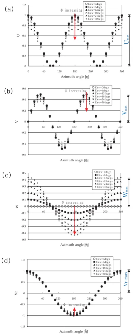
Fig. 10. Variations of the transformed velocity componentsU (a),

V (b) and W (c) and radial velocity component V_r (d) obtained by using VAD technique as functions of the azimuth angle, θ, at different elevation angles,φ. The uniform wind velocity profile is taken as a reference wind velocity field.

0 0.5 1 1.5

0 5 10 15 20 25 30

Ele vation angle [ ]

"U

,V

,W

,V

r"

U_max V_max W_max Vr_max U_ref[=1.0]

a0+b0x+c0x2

a1+b1xn

Ф

Fig. 11. Variations of maximums of the transformed velocity

[image:7.595.55.282.65.629.2]

com-ponentsU (circles),V (triangles), andW (squires) and maximum of radial velocity componentV_r(solid line) as functions of the ele-vation angleφ. The uniform wind velocity profile is taken as a ref-erence wind velocity field, which is presented by short-dashed line. Long-dashed lines present polynomial and power-series fittings of the transformed velocity components.

Fig. 10. Variations of the transformed velocity componentsU(a),

V (b) andW (c) and radial velocity componentVr (d) obtained

by using VAD technique as functions of the azimuth angle,θ, at different elevation angles,φ. The uniform wind velocity profile is taken as a reference wind velocity field.

10 H.-C. LIM & D.-I. LEE: Wind Velocity Retrieval Techniques by a Doppler Radar

-1.5 -1 -0.5 0 0.5 1 1.5

0 60 120 180 240 300 360

Azimuth angle [?]

Vr

0.2 0.4 0.6 0.8 1 1.2

0 60 120 180 240 300 360

Azimuth angle [?]

U

-0.6 -0.4 -0.2 0 0.2 0.4 0.6

0 60 120 180 240 300 360

Azimuth angle [?]

V

-0.5 -0.4 -0.3 -0.2 -0.1 0 0.1 0.2 0.3 0.4 0.5

0 60 120 180 240 300 360

Azimuth angle [?]

W

Θ

Θ Θ

Φ increasing

U

max

V

max

W

max

Vr

-max

( )a

( )b

( )c

( )d

Fig. 10. Variations of the transformed velocity componentsU(a),

V (b) andW (c) and radial velocity componentV_r (d) obtained by using VAD technique as functions of the azimuth angle, θ, at different elevation angles,φ. The uniform wind velocity profile is taken as a reference wind velocity field.

0 0.5 1 1.5

0 5 10 15 20 25 30

"U

,V

,W

,V

r"

U_max V_max W_max Vr_max U_ref[=1.0]

a0+b0x+c0x2

a1+b1xn

Ф

com-ponentsU(circles),V (triangles), andW (squires) and maximum of radial velocity componentVr(solid line) as functions of the ele-vation angleφ. The uniform wind velocity profile is taken as a ref-erence wind velocity field, which is presented by short-dashed line. Long-dashed lines present polynomial and power-series fittings of the transformed velocity components.

com-ponentsU(circles),V (triangles), andW (squires) and maximum of radial velocity componentVr(solid line) as functions of the

ele-vation angleφ. The uniform wind velocity profile is taken as a ref-erence wind velocity field, which is presented by short-dashed line. Long-dashed lines present polynomial and power-series fittings of the transformed velocity components.

the red arrow at the first diagram in Fig. 10. Conversely, the crosswise wind velocity component,V, approaches closer to the reference value of 0 at all azimuth angles as the elevation angle increases. These changes are shown by the red arrow at the second diagram in Fig. 10. The exceptions are two values of azimuth angles of 0◦and 180◦, where the crosswise wind velocity component remains constant and equal to the refer-ence value of 0 at all times. However, the greatest changes produced by changing the elevation angle are observed in the vertical wind velocity component,W. As the elevation angle increases, W progressively deflects from the reference value of 0 at all azimuth angles, except at those of 90◦and 270◦. These changes are shown by the red arrow at the third dia-gram in Fig. 10.

(8)

H.-C. LIM & D.-I. LEE: Wind Velocity Retrieval Techniques by a Doppler Radar

11

-1 -0.8 -0.6 -0.4 -0.2 0 0.2 0.4 0.6 0.8 1

0 60 120 180 240 300 360

Azimuth angle [?]

Vr

Elev=0degs Elev=6degs Elev=12degs Elev=18degs Elev=24degs Elev=30degs -0.5

-0.4 -0.3 -0.2 -0.1 0 0.1 0.2 0.3 0.4 0.5

0 60 120 180 240 300 360

Azimuth angle [?]

W

-0.3 -0.2 -0.1 0 0.1 0.2 0.3 0.4

0 60 120 180 240 300 360

Azimuth angle [?]

V

0.1 0.2 0.3 0.4 0.5 0.6 0.7 0.8

0 60 120 180 240 300 360

Azimuth angle [ ]

U

Θ Θ

Φ increasing

U

max

V

max

W

max

V

r-max

Θ Θ

( )

a

( )

b

( )

c

[image:8.595.53.283.63.627.2]

( )

d

Fig. 12. Same as in Fig. 10 but for the parabolic wind velocity

profile.

0 0.5 1

0 5 10 15 20 25 30

"U

,V

,W

,V

r"

U_max V_max W_max Vr_max U_ref line

a1+b1xn

[image:8.595.312.544.63.223.2]

Ф

profile.

Fig. 14. Flowchart for using the function fitting the

trans-formed velocity components in spherical coordinate system.

profile.

-1 -0.8 -0.6 -0.4 -0.2 0 0.2 0.4 0.6 0.8 1

0 60 120 180 240 300 360

Azimuth angle [?]

Vr

-0.5 -0.4 -0.3 -0.2 -0.1 0 0.1 0.2 0.3 0.4 0.5

0 60 120 180 240 300 360

Azimuth angle [?]

W

-0.3 -0.2 -0.1 0 0.1 0.2 0.3 0.4

0 60 120 180 240 300 360

Azimuth angle [?]

V

0 0.1 0.2 0.3 0.4 0.5 0.6 0.7 0.8

0 60 120 180 240 300 360

Azimuth angle [ ]

U

Θ Θ

Φ increasing

U

max

V

max

W

max

V

r-max

Θ Θ

( )a

( )b

( )c

( )d

profile.

0 0.5 1

0 5 10 15 20 25 30

"U

,V

,W

,V

r"

U_max V_max W_max Vr_max U_ref line

a1+b1xn

Ф

profile.

Figure 12 presents the streamwise, (a), crosswise, (b), and vertical, (c), wind velocity components together with radial wind velocity, (d), as functions of azimuth obtained by appli-cation of the VAD technique to the parabolic reference wind velocity distribution. In this case, as already noted above, the streamwise wind velocity component,U, is equal to 0 near to the ground and gradually increases up to value of 2 at the height 4z/D=2. In addition, as a result of the differ-ent reference wind velocity distribution, the radial velocity is relatively smaller than that in the case of the uniform ref-erence wind velocity. A strong focus should be given here on the crucial role of the reference wind velocity distribution in accuracy of the analysis scheme of the real radar scans. It may be seen from Fig. 12 that sinusoidal variations with azimuth angle are observed in all three wind velocity com-ponents at all elevations considered. Moreover, as the eleva-tion angle increases, the maximums of all three wind velocity components increase significantly. The directions of changes in maximums of all wind velocity components are shown by the red arrows at the first three diagrams in the figure. The maximum of the radial velocity decreases up to 0.8 as the elevation angle increases from 0◦ to 30◦. Figure 13 shows the changes in maximums of the calculated streamwise (cir-cles), crosswise (triangles) and vertical (squares) wind veloc-ity components at azimuth angles of 0◦, 45◦and 0◦, respec-tively, as functions of the elevation angle when the parabolic wind velocity distribution is applied as a reference field. As with the case of the uniform wind velocity distribution, the increase in wind velocity with elevation may be fit by ei-ther a polynomial or power series equation. Three generated general power-series fittings as applied toU,V andW are presented in Fig. 13 by long-dashed lines.

Although the results presented up to now may be seen as a simple comparison with the reference wind velocity, it is clear that an important reduction in the measurement errors

(9)

H.-C. Lim and D.-I. Lee: Wind velocity retrieval techniques by a Doppler radar 659 H.-C. LIM & D.-I. LEE: Wind Velocity Retrieval Techniques by a Doppler Radar 11

-1 -0.8 -0.6 -0.4 -0.2 0 0.2 0.4 0.6 0.8 1

0 60 120 180 240 300 360

Azimuth angle [?]

Vr Elev=0degs Elev=6degs Elev=12degs Elev=18degs Elev=24degs Elev=30degs -0.5 -0.4 -0.3 -0.2 -0.1 0 0.1 0.2 0.3 0.4 0.5

0 60 120 180 240 300 360

Azimuth angle [?]

W Elev=0degs Elev=6degs Elev=12degs Elev=18degs Elev=24degs Elev=30degs -0.4 -0.3 -0.2 -0.1 0 0.1 0.2 0.3 0.4

0 60 120 180 240 300 360

Azimuth angle [?]

V Elev=0degs Elev=6degs Elev=12degs Elev=18degs Elev=24degs Elev=30degs 0 0.1 0.2 0.3 0.4 0.5 0.6 0.7 0.8

0 60 120 180 240 300 360

Azimuth angle [ ]

U Elev=0degs Elev=6degs Elev=12degs Elev=18degs Elev=24degs Elev=30degs Θ Θ Φ increasing Φ increasing Φ increasing Φ increasing U max V max W max V r-max Θ Θ

( )a

( )b

( )c

( )d

profile.

0 0.5 1

0 5 10 15 20 25 30

"U ,V ,W ,V r" U_max V_max W_max Vr_max U_ref line

a1+b1xn

Ф

profile.

4x/D

-2 -1 0 1 2

4y /D -2 -1 0 1 2 PARABOLIC /VAD PARABOLIC /VARD 4x/D

-2 -1 0 1 2

4y /D -2 -1 0 1 2

U: 00.1 0.2 0.3 0.4 0.5 0.6 0.7 0.8 0.9 1

UNIFORM /VAD

UNIFORM /VARD

Fig. 15. Plane Position Indicator (PPI) scan at the height4z/D=

0.1obtained by VAD (upper half of plot) and VARD (lower half of plot) techniques. Uniform (a) and parabolic (b) reference wind velocity distributions applied.

4x/D

-2 -1 0 1 2

4y /D -2 -1 0 1 2

U: 00.1 0.2 0.3 0.4 0.5 0.6 0.7 0.8 0.9 1

4x/D

-2 -1 0 1 2

4y /D -2 -1 0 1 2 PARABOLIC /VAD PARABOLIC /VARD

Fig. 16. Same as in Fig. 15 but at the height4z/D= 0.5.

4x/D

-2 -1 0 1 2

4y /D -2 -1 0 1 2

U: 00.1 0.2 0.3 0.4 0.5 0.6 0.7 0.8 0.9 1

UNIFORM /VAD UNIFORM /VARD 4x/D -2 -1 0 1 2 4y/D -2 -1 0 1 2 U 0 0.5 1

U:00.1 0.2 0.3 0.4 0.5 0.6 0.7 0.8 0.91

4x/D -2 -1 0 1 2 4y/D -2 -1 0 1 2 U 0 0.5 1

Fig. 18. Comparison of Plane Position Indicator (PPI) scan of

streamwise velocity component (a) with trans-function fitted by fourth-order regression at the height4z/D= 0.5and uniform ref-erence wind velocity distribution.

Fig. 15. Plane Position Indicator (PPI) scan at the height 4z/D=0.1

obtained by VAD (upper half of plot) and VARD (lower half of plot) techniques. Uniform (a) and parabolic (b) reference wind velocity distributions applied.

can be produced with the proper representation of the calcu-lated changes in all wind velocity components. Therefore, it is logically to find a mechanism for transforming the cal-culated values of the wind velocity components to real pre-assumed value. One such ways is using transformation func-tions.

3.3 Transformation function

Transformation functionsF (hereafter trans-functions) may be used to transform the shape of the calculated wind velocity componentsU,V andW as obtained by using VAD/VARD

4x/D

-2 -1 0 1 2

4y /D -2 -1 0 1 2

U: 0 0.1 0.2 0.3 0.4 0.5 0.6 0.7 0.8 0.9 1

Fig. 15. Plane Position Indicator (PPI) scan at the height4z/D =

4x/D

-2 -1 0 1 2

4y /D -2 -1 0 1 2

U: 0 0.1 0.2 0.3 0.4 0.5 0.6 0.7 0.8 0.9 1

4x/D

-2 -1 0 1 2

4x/D

-2 -1 0 1 2

4y /D -2 -1 0 1 2

U: 0 0.1 0.2 0.3 0.4 0.5 0.6 0.7 0.8 0.9 1

4x/D -2 -1 0 1 2 4y/D -2 -1 0 1 2 U 0 0.5 1

U:00.1 0.2 0.3 0.4 0.5 0.6 0.7 0.8 0.91

4x/D -2 -1 0 1 2 4y/D -2 -1 0 1 2 U 0 0.5 1

Fig. 16. Same as in Fig. 15 but at the height 4z/D=0.5.

4x/D

-2 -1 0 1 2

4y /D -2 -1 0 1 2

U: 00.1 0.2 0.3 0.4 0.5 0.6 0.7 0.8 0.9 1

Fig. 15. Plane Position Indicator (PPI) scan at the height4z/D=

0.1 obtained by VAD (upper half of plot) and VARD (lower half of plot) techniques. Uniform (a) and parabolic (b) reference wind velocity distributions applied.

4x/D

-2 -1 0 1 2

4y /D -2 -1 0 1 2

U: 00.1 0.2 0.3 0.4 0.5 0.6 0.7 0.8 0.9 1

4x/D

-2 -1 0 1 2

4x/D

-2 -1 0 1 2

4y /D -2 -1 0 1 2

U: 00.1 0.2 0.3 0.4 0.5 0.6 0.7 0.8 0.9 1

4x/D -2 -1 0 1 2 4y/D -2 -1 0 1 2 U 0 0.5 1

U:00.1 0.2 0.3 0.4 0.5 0.6 0.7 0.8 0.91

4x/D -2 -1 0 1 2 4y/D -2 -1 0 1 2 U 0 0.5 1

Fig. 17. Same as in Fig. 15 but at the height 4z/D=1.0.

4x/D

-2 -1 0 1 2

4y /D -2 -1 0 1 2

U: 00.1 0.2 0.3 0.4 0.5 0.6 0.7 0.8 0.91

Fig. 15. Plane Position Indicator (PPI) scan at the height4z/D =

4x/D

-2 -1 0 1 2

4y /D -2 -1 0 1 2

U: 00.1 0.2 0.3 0.4 0.5 0.6 0.7 0.8 0.91

4x/D

-2 -1 0 1 2

4x/D

-2 -1 0 1 2

4y /D -2 -1 0 1 2

U: 00.1 0.2 0.3 0.4 0.5 0.6 0.7 0.8 0.91

4x/D -2 -1 0 1 2 4y/D -2 -1 0 1 2 U 0 0.5 1

U:00.1 0.2 0.3 0.4 0.5 0.6 0.7 0.8 0.91

4x/D -2 -1 0 1 2 4y/D -2 -1 0 1 2 U 0 0.5 1

streamwise velocity component (a) with trans-function fitted by fourth-order regression at the height 4z/D=0.5 and uniform ref-erence wind velocity distribution.

techniques into the required shape in a specific pseudo-domain by tracing the values of the real velocity components. The procedure which is summarized in the flow chart shown in Fig. 14 includes: (i) generation of the virtual domain and allocation of the input velocity; (ii) computation of the ra-dial velocity by using VAD/VARD techniques; (iii) compar-ison of the real and transformed velocities; and, finally (iv) evaluation of the possible trans-functions reducing the errors. Note that the spherical coordinate system fixed with the radar in origin usually leads a biased interpretation of the veloc-ity components so that the true values can be obtained indi-rectly by using a systematic three-dimensional curve-fitting scheme. In addition, the comparison between the flow field obtained by the trans-function and the values of real wind

(10)

( ) 4th order regressiona (b) 6th order regression

(c) 8th order regression (d) 10th order regression

0 0.5 1 1.5 2 2.5

0 0.5 1 4x/D 1.5 2 2.5

4z/

D

VAD

VARD

U=U'/F

Uref=1.0

0 0.5 1 1.5 2 2.5

4x/D

4z/

D

VAD

VARD

U=U'/F

Uref=1.0

0 0.5 1 1.5 2 2.5

4x/D

4z/

D

VAD

VARD

U=U'/F

Uref=1.0

0 0.5 1 1.5 2 2.5

0 0.5 1 _4x/D 1.5 2 2.5

4z/

D

VAD

VARD

U=U'/F

[image:10.595.99.494.65.475.2]

Uref=1.0

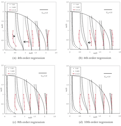
Fig. 19. Comparison of the profiles of streamwise velocity

compo-nent along the centerline by using VARD scheme and fitted data by fourth- to tenth-order regressions.

Fig. 19. Comparison of the profiles of streamwise velocity component along the centerline by using VARD scheme and fitted data by

fourth-to tenth-order regressions.

velocity may predict the error arising from the coordinate transform.

Figures 15, 16 and 17 show the contours of the stream-wise wind velocity component obtained by VAD (upper half of plot) and VARD (lower half of plot) techniques to the uni-form (left-hand side) and parabolic (right-hand side) refer-ence wind velocity distributions at the heights of 4z/D=0.1, 0.5 and 1.0, respectively. This type of presentation is called Plane Position Indicator (PPI) plot. The direction of wind flow in the presented PPI plots is from left to right. A typical sinusoidal coordinate transform from the radial velocity may be applied to obtain the streamwise wind velocity compo-nent. In spherical coordinate system, the plane of symmetry is based on the vertical centerline so to get entire picture it would be sufficient to show only a half of the plot for the

specific method and specific reference wind velocity assum-ing the symmetry for the second half.

As it may be seen in Fig. 15, at the height of 4z/D=0.1 , i.e. very close to the ground level, the streamwise veloc-ity component predicts the reference wind velocveloc-ity relatively well, remaining in the range of 10% error within the sectors covered by the azimuth ranges from 335◦ _{to 25}◦_{and from} 155◦_{to 205}◦_{. Out of those ranges, however, the coincidence} is very poor and gets even worse as one gets further out of the mentioned azimuth ranges. Comparing this PPI plot with the PPI plots at other heights, such as in Figs. 16 and 17, it may be concluded that the above mentioned ranges of good co-incidence permanently narrows at the higher level. As com-pared to the VAD method, the VARD method gives relatively better result in the central domain along the vertical line.