www.hydrol-earth-syst-sci.net/13/2399/2009/ © Author(s) 2009. This work is distributed under the Creative Commons Attribution 3.0 License.
Earth System
Sciences
Reducing scale dependence in TOPMODEL using a dimensionless
topographic index
A. Ducharne
Laboratoire Sisyphe, CNRS/UPMC, Paris, France
Received: 28 January 2009 – Published in Hydrol. Earth Syst. Sci. Discuss.: 4 March 2009 Revised: 6 November 2009 – Accepted: 10 November 2009 – Published: 14 December 2009
Abstract. This paper stems from the fact that the topo-graphic index used in TOPMODEL is not dimensionless. In each pixeli in a catchment, it is defined asxi=ln(ai/Si),
whereai is the specific contributing area per unit contour
length andSi is the topographic slope. In the SI unit system,
ai/Si is in meters, and the unit ofxiis problematic. We
pro-pose a simple solution in the widespread cases where the to-pographic index is computed from a regular raster digital ele-vation model (DEM). The pixel lengthCbeing constant, we can define a dimensionless topographic indexyi=xi−lnC.
Reformulating TOPMODEL equations to useyiinstead ofxi
helps giving the units of all their terms and emphasizes the scale dependence of these equations via the explicit use ofC outside from the topographic index, in what can be defined as the transmissivity at saturation per unit contour lengthT0/C.
The term lnC defines the numerical effect of DEM resolu-tion, which contributes to shift the spatial meanxof the clas-sical topographic index when the DEM cell sizeCvaries. A key result is that both the spatial meanyof the dimensionless index andT0/C are much more stable with respect to DEM
resolution than their counterparts x and T0 in the classical
framework. This shows the importance of the numerical ef-fect in the dependence of the classical topographic index to DEM resolution, and reduces the need to recalibrate TOP-MODEL when changing DEM resolution.
1 Introduction
TOPMODEL was originally introduced by Beven and Kirkby (1979) as a conceptual rainfall-runoff model, describ-ing the contributions of both saturation excess flow and base-flow from the saturated zone to the catchment outbase-flow.
Sim-Correspondence to: A. Ducharne
plifying assumptions, widely known as TOPMODEL’s as-sumptions, allow one to relate the spatial distribution of the water table depth to the one of a topographic index (TI), de-pending in each point of the catchment upon local slope, up-slope contributing area, and downup-slope contour length. This distribution of the water table depth controls (i) baseflow ow-ing to the physically-based Darcy’s law, and (ii) the extent of the surface saturated area, thus the saturation excess flow, owing to the variable contributing area concept first proposed by Cappus (1960).
This model has been widely used, and not only as a rainfall-runoff model. As high values of the TI reflect a high potential for local saturation, maps of this index have been used to delineate wetlands (e.g. M´erot et al., 1995; Curie et al., 2007). Over the last decade, TOPMODEL’s concepts have also been increasingly used in land surface models to describe the influence of topography on the lateral hetero-geneity of runoff, soil moisture, and the coupled surface en-ergy balance, including evapotranspiration (e.g. Famiglietti and Wood, 1994; Peters-Lidard et al., 1997; Stieglitz et al., 1997; Koster et al., 2000; Ducharne et al., 2000; Chen and Kumar, 2001; Decharme and Douville, 2006).
The high popularity of TOPMODEL arises from its sim-plicity of use, especially since topography has become widely described by digital elevation models (DEMs) from which it is easy to compute the TI. A recurring issue, how-ever, is that the TI distribution is markedly impacted by the topographic information content of DEMs, which depends both on the scale of the topographic map the DEM is derived from (Wolock and Price, 1994), and on the DEM resolution, as defined by the pixel size.
(2000); Wu et al. (2007). This increase in mean TI has important hydrological consequences since it imposes to si-multaneously decrease the effective value of transmissivity to preserve the hydrological performance of TOPMODEL, as first showed by Franchini et al. (1996) and detailed in Sect. 4.1. In this framework, many efforts have dealt with detailed geomorphological analyses to understand the com-plex relationships between DEM resolution and the TI or its components, namely the local slope and the specific upslope contributing area (e.g. Wolock and Price, 1994; Sørensen and Seibert, 2007), and to formalize these empirical relationships into scaling functions (e.g. Saulnier et al., 1997b; Wolock and McCabe, 2000; Ibbitt and Woods, 2004; Pradhan et al., 2006).
This paper addresses the scaling issues related to the TI from a different perspective. A reminder of the TOPMODEL framework in Sect. 2 leads us to the starting point of this anal-ysis: the TI is not dimensionless but it is the logarithm of a ratio dimensioned in meters. In Sect. 3, we show how this ra-tio explicitly depends on DEM resolura-tion when topography is described by a raster DEM, as in most present time ap-plications of TOPMODEL. We further show how we can de-fine a dimensionless TI, which is free from this mathematical dependence, and how we can easily rearrange the equations of TOPMODEL to use this dimensionless TI. This does not change TOPMODEL at all, but this new formalism helps to better understand the scale issues in TOPMODEL, as shown in Sect. 4, from a theoretical point of view, then based on real-world case studies, then by comparison with published rescaling techniques.
2 Classical TOPMODEL’s development
The following development of TOPMODEL equations from its simplifying assumptions is not new and was inspired by many papers, in particular from Beven and Kirkby (1979), Sivapalan et al. (1987), Franchini et al. (1996) and Stieglitz et al. (1997). All notations are defined in Table 1 with their SI unit.
2.1 Scope and assumptions
Let us consider a hydrological catchment of area A. Let us further assume that the topography of this catchment is described by a raster DEM with a pixel length C so that A=nC2,nbeing the number of pixels in the catchment.
To describe the evolution of the water table depth over time and space, which is crucial to predict baseflow from this wa-ter table and the extent of saturated areas thus saturation ex-cess flow, TOPMODEL relies on four strong assumptions H1 to H4 regarding the behaviour of the modelled catchment: H1: at each time step, the recharge to the water table,R(t ),
is uniform in the catchment.
H2: the water table dynamics is approximated by a succes-sion of steady states, so that in each pixel of the catch-ment and at each time step, the local outflow from the saturated zone equals the recharge from the contributing area. Isolating one time step, over which the uniform recharge rate isR, we can thus writeQi, the outflow
from the saturated zone at any pixeliin the catchment, as
Qi=AiR (1)
whereAi is the local contributing area.
H3: in each pixeli, the local hydraulic gradient is approxi-mated by the local topographic slopeSi.
H4: the saturated hydraulic conductivityKsis uniform in the
catchment but decreases with depth following an expo-nential law:
Ks(z)=K0exp(−νz) (2)
wherezis the depth from the soil surface,K0=Ks(z=
0)is the saturated hydraulic conductivity at the soil sur-face, andν is the saturated hydraulic conductivity de-cay factor with depth. BothK0andνare uniform in the
catchment.
Assumption H4 has been relaxed by Ambroise et al. (1996) and Duan and Miller (1997) regarding the shape of the verti-cal profile of saturated hydraulic conductivity, and by Beven (1986) regarding the uniformity ofK0. Assumption H2 has
been relaxed by Beven and Freer (2001a) using a kinematic wave routing of subsurface flow. Assumption H3, pertaining to the local hydraulic gradient, can also be relaxed, using the concept of reference levels (Quinn et al., 1991). Assumption H1, however, is essential to derive the simple relationship be-tween the local and mean water depths which is at the crux of TOPMODEL (Eq. 13). The only way to relax it is to separate different landscape or hillslope elements within the catch-ment, as already proposed in the seminal paper by Beven and Kirkby (1979) and further developed in the finely distributed application of TOPMODEL of Peters-Lidard et al. (1997). For simplicity, we will stick in the following to the original assumptions.
2.2 Towards TOPMODEL equations
From Darcy’s law and assumption H3, the local outflow from the saturated zone at pixel i, across a downstream edge of lengthLi, can be written
Qi=LiTiSi. (3)
In this expression,Tiis the local transmissivity defined as
Ti=
Z ∞
zi
Table 1. Notations and units (pertaining to Sects. 2 and 3.1).
Variable SI unit Description
ai m Specific contributing area per unit contour length
aout m Specific contributing area per unit contour length at the outlet (aout=A/Lout)
A m2 Catchment area
Ai m2 Contributing area at pixeli C m DEM resolution (pixel length)
hi m Local altitude at pixeli
Ks m s−1 Saturated hydraulic conductivity
K0 m s−1 Saturated hydraulic conductivity at the surface Li m Downhill contour length at pixeli
Lout m Downhill contour length at the outlet pixel n – Number of pixels in the catchment
ni – Local number of upslope pixels at pixeli
nout – Local number of upslope pixels at the outlet (n=nout) pi m Local piezometric head at pixeli
Qi m3s−1 Outflow from the saturated zone at pixeli
Qout m3s−1 Outflow from the saturated zone at the outlet, or baseflow from the catchment R m s−1 Uniform recharge rate in the catchment
Si – Local topographic slope at pixeli Sout – Local topographic slope at the outlet
Ti m2s−1 Local transmissivity of the saturated zone at pixeli
T0 m2s−1 Local transmissivity at saturation, assumed uniform in the catchment (H4) xi ln(m) Classical topographic index at pixeli
xout ln(m) Classical topographic index at the outlet
x ln(m) Catchment average of the classical topographic index
yi – Dimensionless topographic index at pixeli yout – Dimensionless topographic index at the outlet
y – Catchment average of the dimensionless topographic index
zi m Local water table depth at pixeli zout m Local water table depth at the outlet z m Catchment average of the water table depth
ν m−1 Saturated hydraulic conductivity decay factor with depth
wherezi is the local depth to the water table. Combining
with Eq. (2), we get Ti=K0
Z ∞
zi
e−νzdz=K0
ν exp(−νzi)=T0exp(−νzi) (5) whereT0=K0/νis the transmissivity of the soil when it is
fully saturated (zi=0). Combining Eqs. (1), (3) and (5) leads
to
Qi=AiR=LiT0Siexp(−νzi). (6)
Under TOPMODEL’s assumptions, this holds everywhere in the catchment, in particular at the outlet which drains the en-tire catchment. The baseflow from the catchment is thus Qout=LoutT0Soutexp(−νzout) (7)
where the only unknown iszout, the water table depth at the
outlet pixel where the local slope is Sout. More generally,
the distribution of the local water table depthziin the
catch-ment is used to deduce the surface saturated area, which is defined by the pixels wherezi≤0. Rewriting Eq. (6),zi can
be expressed as follows: zi= −
1 νln
AiR
LiT0Si
. (8)
Introducingai=Ai/Li, the specific contributing area per unit
contour length, we find the classical TOPMODEL equation, where the fraction in the natural logarithm is dimensionless: zi= −
1 νln
aiR
T0Si
. (9)
Separating, in the natural logarithm, the variables that are uniform in the catchment from the ones that are not, we get zi= −
1 ν
lnR T0
+lnai Si
The variable term is defined in TOPMODEL as the topo-graphic index (TI):
xi=ln
ai
Si
. (11)
Note that relaxing the assumption thatK0is uniform leads
to another index of lateral heterogeneity (Beven, 1986), the soil-topographic index ln(ai/TiSi). In any case, the ratio on
which the natural logarithm is applied is not dimensionless. The mean water table depthzis introduced to eliminate the uniform term:
z= −1 ν
ln(R T0
)+x
(12) so that
zi−z= −
1
ν(xi−x) (13)
wherex is the average ofxi over the catchment. This
equa-tion, which states that the spatial variations of the water table and the TI are proportional, is probably the most important in the TOPMODEL framework. It is used to deduce the surface saturated area from the distribution of xi in the catchment
and the mean table depthz. Applied to the outlet pixel, with local water table depth and TIzoutandxout, it also gives
zout=z−
1
ν(xout−x) (14)
which, substituted in Eq. (7), leads to Qout=LoutT0Soutexp(−νz+xout−x)
=LoutT0Soutexp(ln
aout
Sout
)exp(−νz−x)
=aoutLoutT0exp(−νz−x)
Qout=AT0exp(−νz−x). (15)
Using SI units, AT0 is in m4s−1, but Qout is in m3s−1.
This results from the fact that exp(−x)is in m−1, sincexi
is the natural logarithm of a ratio dimensioned in m. Even if Eqs. (10), (12), (13) and (15) are homogeneous, using the logarithm of a non-dimensionless quantity as an index might be confusing. We thus introduce a dimensionless TI, which solves this dimension issue and helps to understand the scale issues related to DEM resolution, as developed in the follow-ing.
3 Introducing a dimensionless TI
3.1 Topographic analysis using single-flow direction algorithms
Many methods are available for deriving the slopesSi,
up-slope contributing areas Ai, and downhill contour length
Li, from a regular raster DEM. The most simple ones are
the single-flow direction (SFD) algorithms, according to which one pixel contributes to only one downslope pixel (e.g. Wolock and Price, 1994). These algorithms rely on the digi-tal terrain analysis (DTA) methods introduced by Jenson and Domingue (1988) and are still very popular (e.g. Wolock and McCabe, 2000; Kumar et al., 2000). In this framework, hav-ing definedCas the DEM cell size thus pixel length, we can write thatLi=C andAi=niC2, whereni is the number of
pixels in the contributing area. This leads to xi=ln
niC
Si
. (16)
The pixel lengthCbeing a constant, we can thus introduce a dimensionless topographic index
yi=ln
ni
Si
(17) which simply relates toxi
xi=yi+lnC. (18)
Dimensionless does not mean scale independent and bothyi
andxi depend on DEM resolution, which controls ni and
Si (e.g. Wolock and McCabe, 2000; Sørensen and Seibert,
2007). Equation (18), however, shows that the classical TIxi
is subjected to an additional influence from DEM resolution, explicited by the term lnC. This term is responsible of the numerical effect detailed in Sect. 4.1, which contributes to shift the mean classical TIxwhen DEM resolution varies.
Section 3.2 will show how Eqs. (17) and (18) can be gener-alized to the more complex cases where multiple-flow direc-tion algorithms (e.g. Quinn et al., 1991) are used to compute ai,Li andSi. In any case, Eq. (10) becomes
zi= −
1 ν
ln(CR T0
)+yi
(19) where the natural logarithm is applied to two dimensionless terms. In addition, the DEM resolution is explicited viaC.
From there, we can follow the same development with this index as in TOPMODEL withxiand introduce the mean
wa-ter table depthzto eliminate the uniform term: zi−z= −
1
ν(yi−y) (20)
whereyis the average ofyi over the catchment. Applied to
the outlet pixel, it gives zout=z−
1
ν(yout−y) (21)
which, substituted in Eq. (7), leads to Qout=C T0Soutexp(−νz+yout−y)
=C T0Soutexp(ln
nout
Sout
)exp(−νz−y)
Qout=
AT0
C exp(−νz−y). (22)
This expression is of course perfectly equivalent to Eq. (15), except that it relies on a dimensionless TI y, and that the scale dependence of this expression explicitly appears via the DEM cell sizeC.
3.2 Generalization to multiple-flow direction algorithms
Since their introduction by Quinn et al. (1991), multiple-flow direction (MFD) algorithms have been widely used to com-pute the TI and regularly improved (e.g. Holmgren, 1994; Quinn et al., 1995; Seibert and McGlynn, 2006). Their ba-sic difference with SFD algorithms is that they distribute the contribution from the upslope contributing area between all the contiguous downslope cells, proportionally to the corre-sponding slopes.
In this framework, the expression of the specific area drained per unit contour length is not as simple as the one used with SFD methods, what leads to the following general expression of the TI:
xi=ln
Ai Pnd
d=1SidLdi !
, (23)
wherendis the total number of downhill directions,Sidis the
slope between the local pixeli and the neighbouring pixel in thedth downhill direction, and Ldi is the contour length normal to this direction. Note that this expression also holds fornd=1, which corresponds to the SFD case.
There are many other variations around the general ba-sis provided by the SFD and MFD methods (e.g. Mendicino and Sole, 1997; Tarboton, 1997). Alternatives also exist re-garding the way to account for channel or creek pixels (e.g. Saulnier et al., 1997a; Mendicino and Sole, 1997; Sørensen et al., 2006) or the way to determine flow direction and slope in flat areas (e.g. Wolock and McCabe, 1995; Pan et al., 2004; Gascoin et al., 2009). Several papers addressed the compar-ison of the various DTA methods to derive the TI (Wolock and McCabe, 1995; Mendicino and Sole, 1997; Pan et al., 2004; Sørensen et al., 2006). They all demonstrate the sensi-tivity of the TI distribution (including the mean TIx) to these methods, but their conclusions regarding the relative perfor-mances of the different methods are not consistent, apart from a consensus about the superiority of MFD algorithms for divergent hillslopes.
In any case, one can always write thatAi=αiC2andLdi =
βidC, whereαi andβid are dimensionless factors. This leads
to the general form of the TI
xi=ln
αiC Pnd
d=1Sidβid !
(24)
which can be reduced to the dimensionless TI yi=ln
αi Pnd
d=1S d iβ
d i
!
=xi−lnC (25)
owing to the fact that the pixel lengthCis constant in regular raster DEMs.
3.3 Generalization to alternative transmissivity profiles Ambroise et al. (1996) generalized TOPMODEL to use lin-ear and parabolic transmissivity profiles, which, according to the analysis of recession curves by Tallaksen (1995), may be better suited in some cases than the classical exponential pro-file (Eq. 5). Duan and Miller (1997) built upon this work to propose a fully generalized power function for the transmis-sivity profile, that can be formulated as follows:
Ti=T0
1−ν bzi
b
. (26)
The only new variable isb, which is is a non-dimensional parameter, uniform throughout the catchment, introduced to generalize the solution of Ambroise et al. (1996). In this framework, the decrease of T0 with depth is controlled by
the ratioν/brather than byν. This generalized power func-tion contains the full range of potential transmissivities, from linear whenb=1 to exponential whenb→ ∞. The classical topographic index becomes
xi=
a
i
Si 1/b
, (27)
the local water table depthzi follows
1−ν bzi
1−ν bz
=xi
x , (28)
and the baseflow at the outlet of the catchment is Qout=AT0
1−ν
bz
y
b
. (29)
A dimensionless index can also be defined in this generalized framework:
yi=
xi
C1/b, (30)
and the expressions of the local water table depth and base-flow become
1−ν bzi
1−ν bz
=yi
y (31)
and Qout=
AT0
C
1−ν
bz
x
b
, (32)
4 Implications regarding scale issues in TOPMODEL 4.1 Attribution of scale effects on the TI distribution
and TOPMODEL parameters
Following Zhang and Montgomery (1994), Franchini et al. (1996) showed that the increase inx when DEM resolution gets coarser had hydrological consequences, as it had to be offset by larger calibrated transmissivities in TOPMODEL. In a given catchment, two DEMs with different cell sizes C2> C1 correspond to different mean TIsx2> x1, what is
known as the shift effect. If the calibrated value of TOP-MODEL’s transmissivity is T0,1 for cell size C1, the shift
effect can be compensated by a simple recalibration of this transmissivity toT0,2, such as to maintain the relationship
between the mean water table depthz∗ and TOPMODEL’s baseflowQ∗:
Q∗=AT0,1exp(−νz∗−x1)=AT0,2exp(−νz∗−x2). (33)
Following Franchini et al. (1996), we assume constantνfor simplicity. This leads to the following relationship, which explains the interplay between the calibrated transmissivities and mean TIs:
T0,2=T0,1exp(x2−x1). (34)
The dimensionless indexy is very much inspired by this pioneering work of Franchini et al. (1996). It also offers a deeper insight on this important interplay between mean TI and calibrated transmissivity. Applying Eq. (18) reveals the direct influence of the change inConto the change in mean classical TIs:
(x2−x1)=ln
C2
C1
+(y2−y1). (35)
It also allows one to explicitly describe this direct DEM in-fluence in Eq. (34), otherwise unchanged:
T0,2=T0,1
C2
C1
exp(y2−y1), (36)
what leads to generalize this relationship to the transmissivity per unit contour length:
T0,2
C2 =T0,1
C1
exp(y2−y1). (37)
Of course, (y2−y1) also depend on DEM resolution.
Equations (35) and (36) thus show that the changes in mean classical TI x and calibrated T0 when the DEM resolution
varies arise from two different causes, as also summarized in Table 2:
– a numerical effect, because the DEM cell size mathe-maticallyCenters into the expression ofai. Using the
dimensionless TI allows one to identify this numerical effect (Eq. 35), which changesx by ln(C2/C1)andT0
by the scaling factorC2/C1;
– a terrain effect, owing to the influence of DEM resolu-tion on both the local slopesSiand the shape of the
hy-drographic network, thusni andai. Following Wolock
and McCabe (2000), this terrain effect can itself be sep-arated in two components: a discretization effect, which arises from dividing the terrain in different numbers of grid cells; and a smoothing effect, related to decreased variability of the local slopes when using coarser reso-lution DEMs, what filters the terrain roughness (Valeo and Moin, 2000).
These terrain effects, which concern both the classical and dimensionless TI, have consequences on the shape of the TI distribution and on its mean. The effect on the mean contributes to the shift effect, and its consequence on the calibratedT0is isolated in the term exp(y2−y1)
of Eq. (36). Note that this effect also influences the transmissivity per unit contour lengthT0/C, owing to
the interplay between the latter and the mean dimen-sionless TI (Eq. 37).
To summarize this theoretical analysis, the influence of DEM resolution on the shape of the TI distribution is shared by the classical and dimensionless TIs. In contrast,yand the trans-missivity per unit contour lengthT0/Care probably less
sen-sitive to DEM resolution than their counterparts in the clas-sical formulation,xandT0, because the former only depend
on the terrain effects, whereas the latter also depend on the numerical effect. This is further investigated based on real-world case studies.
4.2 Importance of the numerical effect in real-world case studies
In the extensive literature devoted to the influence of DEM resolution onto the classical TI distribution and the perfor-mances of TOPMODEL, we could find six papers allowing us to calculate the mean of the dimensionless indexyfor dif-ferent DEM cell sizesC. The six corresponding case stud-ies are briefly summarized in Table 3. Note that the Mau-rets catchment (Saulnier et al., 1997b) is a subcatchment of the experimental research catchment of the R´eal Collobrier (Franchini et al., 1996), and that mean TIs from two differ-ent DTAs, namely the SFD and MFD algorithms, are avail-able in the sub-catchment W3 of the Sleepers River (Wolock and McCabe, 1995).
In the six case studies, TOPMODEL was calibrated for each of the different tested DEM resolutions, to optimize the fit between predicted and observed discharge. The goodness-of-fit criterion was the Nash and Sutcliffe (1970) efficiency, except in the R´eal Collobrier where it was the correlation coefficient between the simulated and observed discharge. The calibration always addressed the surface saturated hy-draulic conductivityK0, but was not systematic for the other
parameters, namelyν, the decay factor ofK0with depth, and
Table 2. DEM resolution effects in the classical TOPMODEL framework: separation of the different effects on the TI distribution, and
quantification of the related changes in mean TIxvs. transmissivityT0. Following Eqs. (36) and (35), the grid cell size is assumed to vary fromC1toC2, with subsequent changes in the mean dimensionless TI fromy1toy2.
DEM resolution effects Influence on TI distribution Quantified effect on
Shape x x T0
(Shift effect)
Numerical × ln(C2/C1) C2/C1
Discretization × ×
Terrain y2−y1 exp(y2−y1)
[image:7.595.53.539.281.374.2]Smoothing × ×
Table 3. Main features of the selected case studies. DTA means Digital Terrain Analysis, and SFD and MFD stand for single and
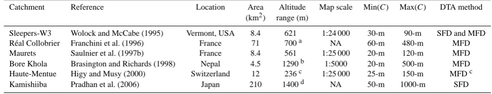
multiple-flow direction algorithms. NA=Not Available.
Catchment Reference Location Area Altitude Map scale Min(C) Max(C) DTA method (km2) range (m)
Sleepers-W3 Wolock and McCabe (1995) Vermont, USA 8.4 621 1:24 000 30-m 90-m SFD and MFD R´eal Collobrier Franchini et al. (1996) France 71 700a NA 60-m 480-m MFD Maurets Saulnier et al. (1997b) France 8.4 561 1:25 000 20-m 120-m MFD Bore Khola Brasington and Richards (1998) Nepal 4.5 1290b 1:5000 20-m 500-m MFD Haute-Mentue Higy and Musy (2000) Switzerland 12 236c 1:25 000 25-m 150-m MFDc Kamishiiba Pradhan et al. (2006) Japan 210 1400d NA 50-m 1000-m SFD
afrom Obled et al. (1994)
bfrom Brasington and Richards (2000) cfrom Iorgulescu and Jordan (1994)
dfrom Lee et al. (2006)
storage, which controls the recharge term in TOPMODEL (Table 4). Important common features of the six calibration exercises are that similar goodness-of-fit were achieved for all DEM resolutions, and thatK0was always the most
effec-tive parameter to compensate the DEM resolution changes, as shown by the small variation ranges, if any, ofνand SR-max in Table 4.
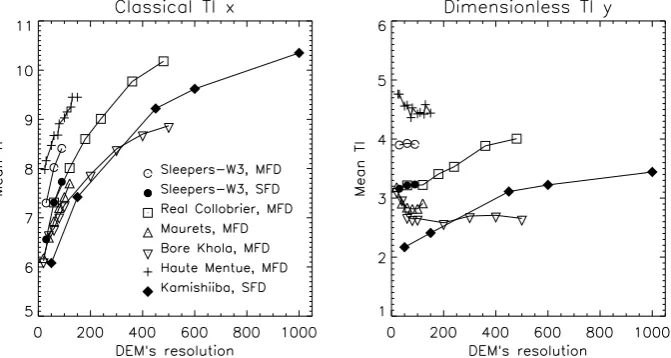
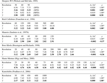
These case studies confirm that, once chosen the DTA method to compute the TI, the mean of the classical index x increases with DEM cell sizeC (Table 5), a rule that we could not find invalidated in the literature. Based on the val-ues gathered in Table 5, the mean classical TIxexhibits vari-ation rates between 0.005 and 0.02, the related unit being ln(m) m−1. In contrast, positive variation rates are not sys-tematic for the mean dimensionless TIy. This analysis also holds for the correlation coefficients of the mean TIs with DEM resolution, which are not systematically positive and high withy, whereas they are significantly so withx.
More importantly, these variation rates show that the mean dimensionless TIy varies much less with DEM resolution than does the mean classical TIx, in all the seven studied cases. This result is further illustrated in Fig. 1, where the
trajectories followed byy span smaller ranges than the ones followed byx under the same DEM resolution changes. Of course, the units are different and there is no point compar-ing x andy for the same DEM resolution. Their changes when DEM resolution varies, however, are important as they motivate the rescaling of transmissivity (Sect. 4.1).
Figure 1 also shows that the variations ofx due to DEM resolution are primarily logarithmic, and exceed the ones re-lated to the DTA methods and the location of the catchments, which controls their specific topographical features. As a re-sult, one cannot isolate the different locations from the vari-ability induced onxby the DEM resolution. In contrast, one can separate the projections of the different trajectories on the vertical axis representingy, what shows that the mean dimensionless TI can efficiently discriminate the different lo-cations, regardless of DEM resolution.
Table 4. Summary of the calibration method and results in the six selected case studies (see Table 3). The goodness-of-fit criterion is
the Nash and Sutcliffe (1970) efficiency, except in the R´eal Collobrier where it is the correlation coefficient between the simulated and observed discharge. In each case, bold figures indicate the parameters that were calibrated to compensate for the DEM resolution changes. NCP=Number of calibrated parameters, NA=Not Available.
Catchment Calibration method Calibration results
Period Time DEM NCP K0range νrange SRmax Efficiency
step resolution (m/h) (m−1) range range
(h) range (m) (mm)
Sleepers-W3 1 year 24 30–90 2 0.018–0.034 3.3–3.6 NA 0.88–0.89
R´eal Collobrier 3 months 1 60–480 1 35–700 58.8 22 0.96*
Maurets 11 storms of 0.5 20–120 3 82–1402 38.5–40 19–21 0.83
10 to 24 days
Bore Khola 1 month 0.5 20–500 3 18–198 14–19.2 3.6–5.8 0.72–0.74
Haute-Mentue 28 days 1 25–150 2 27–118 22.8–29.2 20 0.79–0.82
with 2 storms
Kamishiiba 1 storm NA 50–1000 1 86–2858 1.43 1 0.96
of 120 h
[image:8.595.132.468.318.497.2]* Correlation coefficient
Fig. 1. Relationships between mean TI and DEM resolution, in the classical and dimensionless TOPMODEL frameworks. Values come
from Table 5, which also gives the corresponding correlation coefficients.
panels in Fig. 2, however, shows that if care is not taken to use the same DEM resolution when comparing mean TIs between catchments, the relationship between mean TI and altitude range is completely hidden withx whereas it is de-tectable withy.
The above results are linked to the fact that, at least in the selected catchments, the shift effect onx is largely dom-inated by the logarithmic numerical effect, which is absent by construction when using the dimensionless TI. The DEM effects that remain in the variations ofy are the terrain ef-fects (Sect. 4.1), so that it is advisable to study them on this dimensionless TI rather than on the classical one, where they are largely hidden by the numerical effect. This is illustrated in the right panel of Fig. 1, which shows that these terrain
ef-fects have contrasted signatures in the different catchments, with a positive dependence on DEM resolution in only half of them (Sleepers-W3, R´eal Collobrier, Kamishiiba).
The case studies also reveal thatT0/C varies much less
with DEM resolution than its counterpartT0in the classical
framework (Fig. 3 and Table 6). This is a direct consequence of the interplay between mean TI and transmissivity (Eq. 36), given that the terrain effects, quantified by exp(y2−y1), are
small enough compared to the numerical effectC2/C1to be
neglected at first order. As a result, Eq. (37) can be approxi-mated by
T0,2
C2 'T0,1
C1
Table 5. Mean TIsx(in ln(m)) andy(dimensionless) for six different catchments and different DEM resolutions (cell sizes in m). The reported values come from the literature (see Table 3). The last two columns give: the mean variation rates ofxandywith DEM resolution, in ln(m)m−1and m−1, respectively; the Spearman’s rank correlation coefficientsρbetween the mean TIs and DEM resolution, the star indicating a significant correlation at the riskα=0.05.
Sleepers-W3 (Wolock and McCabe, 1995)
Resolution 30 60 90 1/1C ρ
x 6.56 7.31 7.73 (SFD) 0.020 1.00*
y 3.16 3.22 3.23 (SFD) 0.001 1.00*
x 7.30 8.02 8.41 (MFD) 0.019 1.00*
y 3.90 3.93 3.91 (MFD) 0.000 0.50
R´eal Collobrier (Franchini et al., 1996)
Resolution 60 120 180 240 360 480 1/1C ρ
x 7.31 8.01 8.60 9.01 9.77 10.18 0.006 1.00*
y 3.22 3.22 3.41 3.53 3.88 4.00 0.002 1.00*
Maurets (Saulnier et al., 1997b)
Resolution 20 40 60 80 100 120 1/1C ρ
x 6.18 6.60 6.93 7.20 7.42 7.70 0.015 1.00*
y 3.18 2.90 2.84 2.82 2.82 2.91 −0.002 −0.37
Bore Khola (Brasington and Richards, 1998)
Resolution 20 40 60 80 100 200 300 400 500 1/1C ρ
x 6.12 6.67 6.78 7.03 7.26 7.88 8.40 8.70 8.87 0.006 1.00*
y 3.12 2.98 2.69 2.65 2.65 2.58 2.70 2.71 2.66 −0.001 −0.36
Haute-Mentue (Higy and Musy, 2000)
Resolution 25 30 50 60 75 80 100 110 125 130 150 1/1C ρ
x 7.98 8.16 8.47 8.67 8.68 8.91 9.03 9.15 9.25 9.45 9.45 0.011 0.99*
y 4.76 4.76 4.56 4.58 4.36 4.53 4.42 4.45 4.42 4.58 4.44 −0.000 −0.52
Kamishiiba (Pradhan et al., 2006)
Resolution 50 150 450 600 1000 1/1C ρ
x 6.08 7.42 9.22 9.62 10.35 0.005 1.00*
y 2.17 2.41 3.11 3.22 3.44 0.000 1.00*
Note that this does not imply thatT0/Cis independent from
DEM resolution. Among the four catchments where it makes sense to quantify the correlation betweenT0/C and DEM
resolution (catchments with more than three calibratedT0),
two of them exhibit a positive and significant correlation. In one of them, the Maurets catchment, this cannot be simply attributed to the terrain effects, as there is no significant cor-relation between the mean dimensionless indexy and DEM resolution (Table 5). The dependence ofT0on DEM
resolu-tion is actually more complicated than the one ofx ory, as it is a calibrated parameter, with an important related uncer-tainty. As shown using the GLUE (Generalized Likelihood uncertainty Estimation) methodology for instance, calibra-tion does not allow one to identify a unique optimal set of pa-rameters, and in the special case ofT0, equally good results
can be achieved with values ranging over orders of magni-tude (e.g. Beven and Binley, 1992; Freer et al., 1996; Beven and Freer, 2001b; Gallart et al., 2007). Yet, using the
di-mensionless framework reduces the need to recalibrate TOP-MODEL when DEM resolution varies, asT0/Cbecomes an
explicit parameter, namely the transmissivity at saturation per unit contour length (Eq. 22), which depends much less on DEM resolution thanT0despite the above uncertainties.
4.3 Comparison with alternative rescaling techniques 4.3.1 Rescaling of transmissivity
Table 6. Calibrated transmissivityT0(in m2h−1) and its ratio to pixel lengthT0/C(in m h−1) for six different catchments and different DEM resolutions (cell sizes in m). The reported values come from the literature (see Table 3). The last two columns give: the mean variation rates of the parameters with DEM resolution, in m h−1forT0and in h−1forT0/C; the Spearman’s rank correlation coefficientsρbetween the parameters and DEM resolution, the star indicating a significant correlation at the riskα=0.05.
Sleepers-W3 (Wolock and McCabe, 1995)
Resolution 30 60 90 1/1C ρ
T0 0.001 0.002 0.003 (SFD) 3. 10−5 1.00*
T0/C 3.2 10−5 3.7 10−5 3.8 10−5 (SFD) 1. 10−7 1.00*
T0 0.002 0.004 0.005 (MFD) 5. 10−5 1.00*
T0/C 7.0 10−5 6.3 10−5 5.7 10−5 (MFD) −2. 10−7 −1.00*
R´eal Collobrier (Franchini et al., 1996)
Resolution 60 120 180 240 360 480 1/1C ρ
T0 0.60 1.19 2.55 3.40 7.65 11.90 0.027 1.00*
T0/C 0.010 0.010 0.014 0.014 0.021 0.025 0.000 0.94*
Maurets (Saulnier et al., 1997b)
Resolution 20 40 60 80 100 120 1/1C ρ
T0 2.05 4.60 11.23 21.00 21.37 35.05 0.330 1.00*
T0/C 0.10 0.12 0.19 0.26 0.21 0.29 0.002 0.94*
Bore Khola (Brasington and Richards, 1998)
Resolution 20 40 60 80 100 200 300 400 500 1/1C ρ
T0 0.95 1.36 1.67 1.95 2.46 7.07 7.83 11.86 14.03 0.027 1.00*
T0/C 0.048 0.034 0.028 0.024 0.025 0.035 0.026 0.030 0.028 −0.000 −0.23
Haute-Mentue (Higy and Musy, 2000)
Resolution 25 30 50 60 75 80 100 110 125 130 150 1/1C ρ
T0 1.13 1.45 1.57 1.91 2.20 3.95 4.19 4.02 4.35 4.87 5.20 0.033 0.99*
T0/C 0.05 0.05 0.03 0.03 0.03 0.05 0.04 0.04 0.03 0.04 0.03 −0.000 −0.13
Kamishiiba (Pradhan et al., 2006)
Resolution 50 150 450 600 1000 1/1C ρ
T0 6 200 0.204 1.00*
[image:10.595.134.467.461.638.2]T0/C 0.12 0.20 0.000 1.00*
Fig. 2. Relationships between the altitude range (from Table 3) and the mean TIs in the six selected catchments: classical TI on the left panel
Fig. 3. Relationships between transmissivityT0orT0/Cand DEM resolution, in the classical and dimensionless TOPMODEL frameworks. Values come from Table 6, which also gives the corresponding correlation coefficients. Note that two of the six selected catchments (Sleepers-W3 and Kamishiiba) were excluded as their transmissivity values were outside the range covered in the other catchments (respectively much smaller and much larger).
Yet, T0/C, the resulting rescaled transmissivity, is not
completely invariant when DEM resolution varies, because of the calibration uncertainty on the one hand, and because other scale effects are involved on the other hand. The first one is that the mean TIs (whether classical or dimensionless) are also sensitive to terrain effects (related to discretization and smoothing), as analysed in Sect. 4.1. The second one is that the rescaling of transmissivity also compensates for changes in the TI distribution, as shown by Saulnier et al. (1997b) in the Maurets catchment (described in Table 3). These authors eventually proposed an efficient scaling fac-tor forK0, deduced from the differences in TI cumulative
distributions when the DEM resolution changes.
The above scaling factors can be used to guide and facili-tate the required recalibration of transmissivity when chang-ing the DEM resolution, but it was later rather proposed to directly rescale the TI distribution, such as to limit the need to recalibrate the transmissivity.
4.3.2 Rescaling of the TI distribution
From a regression analysis using a sample of 50 quad-rangles of 1◦×1◦ ('7000 km2) in the conterminous USA, Wolock and McCabe (2000) proposed a linear relationship to rescale the mean TIs obtained from a 1000-m resolution DEM (x1000) to values that would correspond to a 100-m
resolution DEM (x100):
x100= −1.957+0.961x1000. (39)
This linear regression is characterized by a high determina-tion coefficient (R2=0.93) and has been widely used (e.g.
Kumar et al., 2000; Ducharne et al., 2000; Niu et al., 2005; Decharme and Douville, 2006). It can easily be extended to the dimensionless TI:
y100=0.525+0.961y1000, (40)
and the smaller y-intercept in Eq. (40) than in Eq. (39) con-firms thaty depends less on DEM resolution thanx, owing to the elimination of the numerical effect of DEM resolution. Figure 1 also suggests that a logarithmic relationship could perform better.
Mendicino and Sole (1997) analysed the simulations of 11 flood events by TOPMODEL in the Turbolo Creek (29 km2, in Italy), using a 30-m resolution DEM, aggregated to coarser resolutions (90-m, 140-m and 270-m). They proposed a lin-ear relationship between the mean TI and a spatial variabil-ity measure (SVM), which describes the topographic infor-mation content of the DEM following Shannon and Weaver (1949), and which depends on DEM resolution by a simple function of the number of grid cells.
This approach was further explored by Ibbitt and Woods (2004) in a 50-km2 catchment in New Zealand, with simi-lar results. These authors also provided evidence of a linear relationship betweenx(C)and log10(C), which is perfectly consistent with the facts thaty=x−lnC (from Eq. 18) and that y undergoes negligible variations with C, as shown in Sect. 4.2. The relationship betweenx(C) and log10(C) is thus verified in the catchments of Table 5, the correlation co-efficient exceeding 0.99 in all seven cases.
TI distribution to such resolution could render possible to use in situ measurements of the saturated hydraulic conductivity K0, which is otherwise forbidden by the interplay between
the DEM resolution, the mean classical TI andK0.
Another method, aiming at rescaling the entire distribu-tion of the classical TI instead of its mean, was proposed by Pradhan et al. (2006, 2008) in the Kamishiiba catchment (Table 3). The TIxi,1scaled at the target cell sizeC1from a
coarser DEM with a cell sizeC2can be expressed as
xi,1=ln
a
i,2IfRC1 Si,1IfNC2
. (41)
In this equation,IfN andIfR describe the terrain discretiza-tion effects on the upslope contributing area and contour length, respectively. They both depend on the two DEM cell sizesC1andC2, and on the numbers of pixels at the coarser
resolution in the upslope contributing area,ni,2, and in the
entire catchment,nout,2. Note that IfR was recently intro-duced in Pradhan et al. (2008) and is neglected in Pradhan et al. (2006). These authors also propose an interesting way to deduce the local slopesSi,1 at the target resolution from
the coarser DEM and a fractal method to introduce steepest slopes. Rearranging Eq. (41), by keeping in mind thatIfN andIfR vary within the catchment, leads to
xi,1=ln
n
i,2IfR Si,1IfN
+lnC1. (42)
This equation is very close to Eq. (18), as the first term in the right-hand side can be seen as a scaled dimensionless TI. It also reveals the three different DEM effects onto the classical TI distribution, previously separated in Table 2. The numeri-cal effect, which has not been explicitly recognized by Prad-han et al. (2006, 2008), is quantified by lnC1. The
discretiza-tion effect originates fromIfN andIfR, and the smoothing effect from the rescaled slopesSi,1. Note that these scaling
techniques can be applied to the dimensionless as well as to the classical TI.
5 Conclusions
Replacingxi, the classical TI of TOPMODEL, by the
di-mensionless TI yi=xi−lnC, leads to reformulate
TOP-MODEL’s main equations, then replaced by Eqs. (20) and (22). The principles and results of TOPMODEL are totally preserved in doing so but this reformulation offers several advantages. It firstly helps giving the units of all the vari-ables (see Table 1), what is lacking in most papers about TOPMODEL, including the most cited ones (e.g. Beven and Kirkby, 1979; Sivapalan et al., 1987), probably by reluctance to use the logarithm of a length as a unit.
More importantly, the dependence of TOPMODEL equa-tions on DEM cell size C becomes explicit, whereas it is hidden in the TI when using the classical formulation. This is a good way to raise awareness of hydrologists about the
scale and resolution issues in the TOPMODEL framework. The mathematical dependence of TOPMODEL equations on C is then shifted from the classical TI, where it is related to the upslope contributing area per unit contour length, to-wards the equation of baseflow (Eq. 22), viaT0/Cwhich can
be defined as the transmissivity at saturation per unit contour length.
Accordingly, the mean dimensionless TI is free from the numerical effect, introduced in Sect. 4.1 as the direct effect of using the cell size in the definition of the classical TI. The influence of DEM resolution on the distribution of the dimen-sionless TI is thus restricted to the terrain effects, which re-sult from terrain information loss at coarser resolutions, and which can be addressed for instance using the scaling meth-ods proposed by Pradhan et al. (2006, 2008).
Nonetheless, based on six real-world case studies from the literature, we provide evidence that the DEM resolution in-fluence on the mean classical TIx is largely dominated by the logarithmic numerical effect (Sect. 4.2). This results has important consequences, as:
– it sheds a new light upon the widely shared assump-tion according to which the dependence of the classical TI on DEM resolution mostly results from changes in terrain information (e.g. Sørensen and Seibert, 2007), which would probably be better identified by first re-moving the first-order numerical effect;
– the mean of the dimensionless TI is less sensitive to DEM resolution than the one of the classical TI, and it can be used as an efficient indicator to compare the topographic features of different catchments, almost re-gardless of DEM resolution;
– the transmissivity at saturation per unit contour length T0/C is also more stable with DEM resolution than
its counterpart T0 in the classical framework. The
need to recalibrate TOPMODEL when DEM resolution changes is thus markedly reduced using the dimension-less framework.
Finally, the dimensionless TI offers an interesting bridge between the two rescaling strategies developed within the classical TOPMODEL framework to reduce recalibration when DEM resolution changes, namely the rescaling of transmissivity and the rescaling of the TI distribution. Acknowledgements. This paper benefited from fruitful discussions with Simon Gascoin and Pierre Ribstein, from the Laboratoire Sisyphe. The author also wishes to thank the editor, Francesc Gallart, and three reviewers, including Jan Seibert and Mike Kirkby, for their insightful comments, which helped a lot to improve the manuscript.
References
Ambroise, B., Beven, K. J., and Freer, J.: Toward a generalization of the TOPMODEL concepts: Topographic indices of hydrological similarity, Water Resour. Res., 32, 2135–2145, 1996.
Beven, K.: Hillslope runoff processes and flood frequency charac-teristics, in: Hillslope processes, edited by: Abrahams, S. D., Allen and Unwin, Boston, USA, 187–202, 1986.
Beven, K. and Freer, J.: A dynamic TOPMODEL, Hydrol. Process., 15, 1993–201, 2001a.
Beven, K. and Freer, J.: Equifinality, data assimilation, and uncer-tainty estimation in mechanistic modelling of complex environ-mental systems, J. Hydrol., 249, 11–29, 2001b.
Beven, K. and Kirkby, M. J.: A physically based variable contribut-ing area model of basin hydrology, Hydrol. Sci. Bull., 24, 43–69, 1979.
Beven, K. J. and Binley, A. M.: The future of distributed models: model calibration and uncertainty prediction, Hydrol. Process, 6, 279–298, 1992.
Brasington, J. and Richards, K.: Interactions between model pre-dictions, parameters and DTM scales for TOPMODEL, Com-put. Geosci., 24, 299–314, doi:10.1016/S0098-3004(97)00081-2, 1998.
Brasington, J. and Richards, K.: Turbidity and suspended sediment dynamics in small catchments in the Nepal Middle Hills, Hydrol. Process., 14, 2559–2574, 2000.
Bruneau, P., Gascuel-Odoux, C., Robin, P., M´erot, P., and Beven, K.: Sensitivity to space and time resolution of a hydrological model using digital elevation data, Hydrol. Process., 9, 69–81, 1995.
Cappus: Etude des lois d’´ecoulement – Application au calcul et `a la prevision des d´ebits, Bassin exp´erimental d’Alrance, La Houille Blanche, 60, 493–520, 1960.
Chen, J. and Kumar, P.: Topographic Influence on the Seasonal and Interannual Variation of Water and Energy Balance of Basins in North America, J. Clim., 14, 1989–2014, 2001.
Curie, F., Gaillard, S., Ducharne, A., and Bendjoudi, H.: Ge-omorphological methods to characterize wetlands at the scale of the Seine watershed, Sci. Total. Environ., 375, 59–68, doi:10.1016/j.scitotenv.2006.12.013, 2007.
Decharme, B. and Douville, H.: Introduction of a sub-grid hydrol-ogy in the ISBA land surface model, Clim. Dyn., 26, 65–78, doi:10.1007/s00382-005-0059-7, 2006.
Duan, J. and Miller, N. L.: A generalized power function for the subsurface transmissivity profile in TOPMODEL, Water Resour. Res., 33, 2559–2562, 1997.
Ducharne, A., Koster, R. D., Suarez, M., Stieglitz, M., and Ku-mar, P.: A catchment-based approach to modeling land surface processes in a GCM – Part 2: Parameter estimation and model demonstration, J. Geophys. Res., 105, 24823–24838, 2000. Famiglietti, J. S. and Wood, E. F.: Multiscale modeling of spatially
variable water and energy balance processes, Water Resour. Res., 30, 3061–3078, 1994.
Franchini, M., Wendling, J., Obled, C., and Todini, E.: Physical in-terpretation and sensitivity analysis of the TOPMODEL, J. Hy-drol., 175, 293–338, 1996.
Freer, J., Beven, K. J., and Ambroise, B.: Bayesian estimation of uncertainty in runoff prediction and the value of data: An ap-plication of the GLUE approach, Water Resour. Res., 32, 2161– 2173, 1996.
Gallart, F., Latron, J., Llorens, P., and Beven, K.: Using internal catchment information to reduce the uncertainty of discharge and baseflow predictions, Adv. Water Resour., 30, 808–823, doi:10.1016/j.advwatres.2006.06.005, 2007.
Gascoin, S., Ducharne, A., Ribstein, P., Carli, M., and Habets, F.: Adaptation of a catchment-based land surface model to the hy-drogeological setting of the Somme River basin (France), J. Hy-drol., 368, 105–116, doi:10.1016/j.jhydrol.2009.01.039, 2009. Higy, C. and Musy, A.: Digital terrain analysis of the Haute-Mentue
catchment an scale effect for hydrological modelling with TOP-MODEL, Hydrol. Earth Syst. Sci., 4, 225–237, 2000,
http://www.hydrol-earth-syst-sci.net/4/225/2000/.
Holmgren, P.: Multiple flow direction algorithms for runoff mod-elling in grid based elevation models: An empirical evaluation, Hydrol. Process., 8, 327–334, 1994.
Ibbitt, R. and Woods, R.: Re-scaling the topographic index to improve the representation of physical pro-cesses in catchment models, J. Hydrol., 293, 205–218, doi:10.1016/j.jhydrol.2004.01.016, 2004.
Iorgulescu, I. and Jordan, J.-P.: Validation of TOPMODEL on a small Swiss catchment, J. Hydrol., 159, 255–273, 1994. Jenson, S. K. and Domingue, J. O.: Extracting topographic
struc-ture from digital elevation data for geographic information sys-tem analysis, Photogramm. Eng. Rem. S., 54, 1593–1600, 1988. Koster, R. D., Suarez, M., Ducharne, A., Stieglitz, M., and Kumar, P.: A catchment-based approach to modeling land surface pro-cesses in a GCM – Part 1: Model structure, J. Geophys. Res., 105, 24809–24822, 2000.
Kumar, P., Verdin, K. L., and Greenlee, S. K.: Basin level statistical properties of topographic index for North America, Adv. Water Resour., 23, 571–578, 2000.
Lee, G., Tachikawa, Y., and Takara, K.: Analysis of Hydrologic Model Parameter Characteristics Using Automatic Global Opti-mization Method, Annals of Disaster Prevention Research Insti-tute, 67–80, 2006.
Mendicino, G. and Sole, A.: The information content theory for the estimation of the topographic index distribution used in TOP-MODEL, Hydrol. Process., 11, 1099–1114, 1997.
M´erot, P., Ezzahar, B., Walter, C., and Aurousseau, P.: Mapping waterlogging of soils using digital terrain models, Hydrol. Pro-cess., 9, 27–34, 1995.
Nash, J. E. and Sutcliffe, J. V.: River flow forecasting through con-ceptual models. 1. A discussion of principles, J. Hydrol., 10, 282–290, 1970.
Niu, G.-Y., Yang, Z.-L., Dickinson, R. E., and Gulden, L. E.: A simple TOPMODEL-based runoff parameterization (SIMTOP) for use in global climate models, J. Geophys. Res., 110, D21 106, doi:10.1029/2005JD006111, 2005.
Obled, C., Wendling, J., and Beven, K.: The sensitivity of hydro-logical models to spatial rainfall patterns: an evaluation using observed data, J. Hydrol., 159, 305–333, 1994.
Pan, F., Peters-Lidard, C. D., Sale, M. J., and King, A. W.: Compar-ison of geographical information systems-based algorithms for computing the TOPMODEL topographic index, Water Resour. Res., 40, W06 303, doi:10.1029/2004WR003069, 2004. Peters-Lidard, C. D., Zion, M. S., and Wood, E. F.: A
Pradhan, N. R., Tachikawa, Y., and Takara, K.: A downscaling method of topographic index distribution for matching the scales of model application and parameter identification, Hydrol. Pro-cess., 20, 1385–1405, 2006.
Pradhan, N. R., Ogden, F. L., Tachikawa, Y., and Takara, K.: Scaling of slope, upslope area and soil water deficit: implications for transferability and regionalization in topo-graphic index modeling, Water Resour. Res., 44, W12 421, doi:0.1029/2007WR006667, 2008.
Quinn, P., Beven, K., Chevallier, P., and Planchon, O.: The predic-tion of hillslope flow paths for distributed hydrological modelling using digital terrain models, Hydrol. Process., 5, 59–79, 1991. Quinn, P., Beven, K., and Lamb, R.: The ln(a/tanB) index: how to
calculate it and how to use it within the TOPMODEL framework, Hydrol. Process., 9, 161–182, 1995.
Saulnier, G.-M., Beven, K., and Obled, C.: Digital elevation analy-sis for distributed hydrological modelling: reducing scale depen-dence in effective hydraulic conductivity values, Water Resour. Res., 33, 2097–2101, 1997a.
Saulnier, G.-M., Obled, C., and Beven, K.: Analytical compensa-tion between DTM grid resolucompensa-tion and effective values of satu-rated hydraulic conductivity within the TOPMODEL framework, Hydrological processes, 11, 1331–1346, 1997b.
Seibert, J. and McGlynn, B. L.: A new triangular multiple flow direction algorithm for computing upslope areas from gridded digital elevation models, Water Resour. Res., 43, W04 501, doi:0.1029/2006WR005128, 2006.
Shannon, C. E. and Weaver, W.: The Mathematical Theory of Com-munication, University of Illinois Press, Urbana, IL, 117 pp., 1949.
Sivapalan, M., Beven, K., and Wood, E. F.: On Hydrologic Simi-larity : 2. A Scaled Model of Storm Runoff Production, Water Resour. Res., 23, 2266–2278, 1987.
Sørensen, R. and Seibert, J.: Effects of DEM resolution on the calculation of topographical indices: TWI and its components, J. Hydrol., 347, 79–89, 2007.
Sørensen, R., Zinko, U., and Seibert, J.: On the calculation of the topographic wetness index: evaluation of different methods based on field observations, Hydrol. Earth Syst. Sci., 10, 101– 112, 2006,
http://www.hydrol-earth-syst-sci.net/10/101/2006/.
Stieglitz, M., Rind, M., Famiglietti, J., and Rosenzweig, C.: An efficient approach to modeling the topographic control of surface hydrology for regional and global modeling, J. Clim., 10, 118– 137, 1997.
Tallaksen, L. M.: A review of baseflow recession analysis, J. Hy-drol., 165, 349–370, doi:10.1016/0022-1694(94)02540-R, 1995. Tarboton, D. G.: A new method for the determination of flow direc-tions and upslope areas in grid digital elevation models, Water Resour. Res., 33, 309–319, 1997.
Valeo, C. and Moin, S. M. A.: Grid-resolution effects on a model for integrating urban and rural areas, Hydrol. Process., 14, 2505– 2525, 2000.
Wolock, D. and McCabe, G.: Differences in topographic charac-teristics computed from 100- and 1000-meter resolution digital elevation model data, Hydrol. Process., 14, 987–1002, 2000. Wolock, D. M. and McCabe, G. J.: Comparison of single and
multi-ple flow direction algorithms for computing topographic param-eters in TOPMODEL, Water Resour. Res., 31, 1315–1324, 1995. Wolock, D. M. and Price, C. V.: Effects of digital elevation model map scale and data resolution on a topography-based watershed model, Water Resour. Res., 30, 3041–3052, 1994.
Wu, S., Li, J. and Huang, G. H.: Modeling the effects of elevation data resolution on the performance of topography-based water-shed runoff simulation, Environ. Modell. Softw., 22, 1250–1260, doi:10.1016/j.envsoft.2006.08.001, 2007.