Educational Policy Studies Dissertations Department of Educational Policy Studies
Fall 10-25-2010
Controlling Type 1 Error Rate in Evaluating
Differential Item Functioning for Four DIF
Methods: Use of Three Procedures for Adjustment
of Multiple Item Testing
Jihye Kim
Georgia State University
Follow this and additional works at:https://scholarworks.gsu.edu/eps_diss Part of theEducation Commons, and theEducation Policy Commons
This Dissertation is brought to you for free and open access by the Department of Educational Policy Studies at ScholarWorks @ Georgia State University. It has been accepted for inclusion in Educational Policy Studies Dissertations by an authorized administrator of ScholarWorks @ Georgia State University. For more information, please [email protected].
Recommended Citation
Kim, Jihye, "Controlling Type 1 Error Rate in Evaluating Differential Item Functioning for Four DIF Methods: Use of Three Procedures for Adjustment of Multiple Item Testing." Dissertation, Georgia State University, 2010.
ACCEPTANCE
This dissertation, CONTROLLING TYPE I ERROR RATE IN EVALUATING DIFFERENTIAL ITEM FUNCTIONING FOR FOUR DIF METHODS: USE OF THREE PROCEDURES FOR ADJUSTMENT OF MULTIPLE ITEM TESTING, by JIHYE KIM, was prepared under the direction of the candidate’s Dissertation Advisory Committee. It is accepted by the committee members in partial fulfillment of the requirements for the degree Doctor of Philosophy in the College of Education, Georgia State University.
The Dissertation Advisory Committee and the student’s Department Chair, as representatives of the faculty, certify that this dissertation has met all standards of excellence and scholarship as determined by the faculty. The Dean of the College of Education concurs.
Chris. T. Oshima, Ph.D. Yu-Sheng Hsu, Ph.D. Committee Chair Committee Member
William Curlette, Ph.D. Sheryl A. Gowen, Ph.D. Committee Member Committee Member
Date
Sheryl A. Gowen, Ph.D.
Chair, Department of Educational Policy Studies
R.W. Kamphaus, Ph.D.
AUTHOR’S STATEMENT
By presenting this dissertation as a partial fulfillment of the requirements for the
advanced degree from Georgia State University, I agree that the library of Georgia State University shall make it available for inspection and circulation in accordance with its regulations governing materials of this type. I agree that permission to quote, to copy from, or to publish this dissertation may be granted by the professor under whose direction it was written, by the college of Education’s director of graduate studies and research, or by me. Such quoting, copying, or publishing must be solely for scholarly purposes and will not involve potential financial gain. It is understood that nay copying form or publication of this dissertation which involves potential financial gain will not be allowed without my written permission.
NOTICE TO BORROWERS
All dissertation deposited in the Georgia University library must be used in accordance with the stipulations prescribed by the author in the preceding statement. The author of this dissertation is:
Jihye Kim
2574 Willow Grove Road Acworth, GA 30101
The director of this dissertation is:
Dr. Chris T. Oshima
Department of Educational Policy Studies College of Education
VITA
Jihye Kim
ADDRESS: 2574 Willow Grove Road Acworth, Georgia 30101
EDUCATION:
Ph.D. 2010 Georgia State University Educational Policy Studies M.S. 2004 Georgia State University
Biostatistics B.S. 1997 Sangji University
Applied Statistics
PROFESSIONAL EXPERIENCE:
2010-Present Doctoral Fellow
Georgia State University, Atlanta, GA 2009-2005 Graduate Research Assistant
Board of Regent, Atlanta, GA 2003-2005 Graduate Research Assistant
Georgia State University, Atlanta, GA
PROFESSIONAL SOCIETIES AND GORGANIZATIONS:
2004-Present National Council on Measurement in Education 2004-Present American Educational Research Association
PRESENTATIONS AND PUBLICATIONS:
Kim, J., Oshima, T. C. (2010, July). Controlling Type I Error Rate in Evaluating Differential Item Functioning for Four DIF Methods: Use of Adjustment of Multiple Item Testing. Paper presented at the annual meeting of the Psychometric Society, Athens, GA.
ABSTRACT
CONTROLLING TYPE I ERROR RATE IN EVALUATING DIFFERENTIAL ITEM FUNCTIONING FOR FOUR DIF METHODS: USE OF THREE PROCEDURES
FOR ADJUSTMENT OF MULTIPLE ITEM TESTING by
Jihye Kim
In DIF studies, a Type I error refers to the mistake of identifying non-DIF items
as DIF items, and a Type I error rate refers to the proportion of Type I errors in a
simulation study. The possibility of making a Type I error in DIF studies is always
present and high possibility of making such an error can weaken the validity of the
assessment. Therefore, the quality of a test assessment is related to a Type I error rate and
to how to control such a rate. Current DIF studies regarding a Type I error rate have
found that the latter rate can be affected by several factors, such as test length, sample
size, test group size, group mean difference, group standard deviation difference, and an
underlying model. This study focused on another undiscovered factor that may affect a
Type I error rate; the effect of multiple testing.
DIF analysis conducts multiple significance testing of items in a test, and such
multiple testing may increase the possibility of making a Type I error at least once. The
main goal of this dissertation was to investigate how to control a Type I error rate using
adjustment procedures for multiple testing which have been widely used in applied
testing conditions; the methods were the Mantel-Haenszel method, the logistic regression
procedure, the Differential Functioning Item and Test framework, and the Lord’s
chi-square test. Then the Bonferroni correction, the Holm’s procedure, and the BH method
were applied as an adjustment of multiple significance testing. The results of this study
CONTROLLING TYPE I ERROR RATE IN EVALUATING DIFFERENTIAL ITEM FUNCTIONING FOR FOUR DIF METHODS: USE OF THREE PROCEDURES
FOR ADJUSTMENT OF MULTIPLE ITEM TESTING by
Jihye Kim
A Dissertation
Presented in Partial Fulfillment of Requirements for the Degree of
Doctor of Philosophy in
Research, Measurement, and Statistics in
the Department of Educational Policy Studies in
the College of Education Georgia State University
Copyright by Jihye Kim
ii
ACKNOWLEDGEMENTS
I have so many people who encouraged and supported me. First of all, I would like to be grateful to my advisor, Dr. Chris T. Oshima, with my whole heart. I can remember when I just started the Ph.D program in the fall semester at the year 2004. I asked her to be my advisor, and she was willing to accept me. Since then it has been almost six years under her advising. She has guided me with her dedication, patience, and profound knowledge all the time. And Dr. Oshima enabled me to complete this
dissertation. I could not have done it without her. Thank you so much! I also want to give my gratitude to my committee members. Thanks to Dr. Sheryl Gowen for her sincerity and encouragement! For Dr. Curlette, I appreciate his support for entire process of my study. My appreciation extended to Dr. Yu-Sheng Hsu for his guidance of my
dissertation. His insightful advice was helpful for me to go right on track!
I would love to thank friends. First, I give my thanks to Vincent. He reviewed my prospectus and provided invaluable comments. It really helped! At the Board of Regent, University System of Georgia, I had been worked for several years as a graduate research assistant. Experience at the BOR was great and inspired me to look into the evaluation area. My specialized major is the Differential Item Functioning. So, the research on the teacher education program at the BOR was kind of new but invaluable experience to me. Specially, I am grateful to give appreciation to Dr. Patricia Paterson, and Dr. Judy Monsaas. For Dr. Paterson, I have learned so much about the project on the alternative teacher preparation program. And I recognize that my research and study would not have been possible without her financial assistance. Dr. Monsaas is such a wonderful person. She has been always encouraged me and kind enough to allow me to do research with her. For our research, when I seek the research topic with teacher retention data, she provided me a clear direction of research. Then we started to do research together and presented the paper at AERA. It was great for me to present at AERA for the first time. I would like to express my gratitude for her support.
iii
TABLE OF CONTENTS
Page
List of Tables ... iv
List of Figures ... vi
List of Abbreviations ... vii
Chapter 1 INTRODUCTION ...1
Background and Research Questions...1
2 LITERATURE REVIEW ...5
Introduction to DIF methods based on statistical criteria ...5
Significance testing to evaluate DIF items ...6
Descriptions of four DIF methods based on significance testing ...7
Type I error rate on DIF ...13
3 METHOD ...18
Study Design ...18
Conditions of Study ...18
Statistical DIF Methods for Simulation Studies ...23
4 RESULTS ...25
Phase I ...30
Phase II...43
5 DISCUSSION ...52
Conclusion and Significance...52
Limitations and Future Research ...54
References ...56
iv
LIST OF TABLES
Table Page
1 Sample size and sample size ratio of non-parametric methods ...20
2 Item Parameters for the 40 items test and the 20 items test ...21
3 False positives and true positives for each item of
Lord’s chi-square test in a 40 items test ...27
4 Difference of b parameter for a 20 items test and a 40 items test ...28
5 Type I error rate and power rate of non-parametric methods
By test length and sample size ...34
6 Type I error rate and power for parametric methods
By test length and sample size ...35
7 Type I error rate for four DIF methods by group difference ...40
8 The Power rate for four DIF methods by group difference ...41
9 Type I error rate / power rate for the MH method
with group difference (20 items test) ...44
10 Type I error rates and power rate for the MH method
with group difference (40 items test) ...45
11 Type I error rate / power rate for logistic regression procedure
With group difference (20 items test) ...47
12 Type I error rate / power rate for logistic regression procedure
v
14 Effect of three adjustment procedures for Lord’s chi-square test
vi
LIST OF FIGURES
Figure Page
1 The item characteristic curve for a dichotomous item ...12
2 Type I error rate for non-parametric methods
based on sample size with 20 items test...31
3 Type I error rate for parametric methods
based on sample size 1000/1000 ...32
4 Type I error rates among four DIF methods
with 1000/1000 sample size ...32
5 The power rate of four DIF methods with 1000/1000
by different DIF magnitude ...36
6 Inflated Type I error rate with group SD difference
For four DIF methods in a 20 items test ...42
7 Inflated Type I error rate with group SD difference
vii
ABBREVIATIONS
BH Benjamini and Hochberg Method
CDIF Compensatory Differential Item Functioning
CMH Cochran Mantel-Haenszel Method
DFIT Differential Functioning of Items and Tests
DIF Differential Item Functioning
DTF Differential Test Functioning
ICC Item Characteristic Curve
IPR Item Parameter Replication
IRT Item Response Theory
MH Mantel-Haenszel Method
NCDIF Non-Compensatory Differential Item Functioning
1 CHAPTER 1
INTRODUCTION
Background and Research Questions
Differential Item Functioning (DIF) identifies items that show different outcomes
in different groups (e.g., reference and focal group). In other words, DIF exists in a test
when examinees of equal ability in different groups, in terms of education, ethnicity, and
race, have different probabilities of correctly answering items in a test (Holland
&Wainer, 1993).
The ultimate goal of a DIF study is to provide a fair opportunity for every
examinee to perform successfully. A number of tests are provided for evaluating
examinees’ knowledge in various groups. If a test favors one group of examinees over
another, the test is considered to be biased. When a test is unbiased, the score can be
strong evidence of what a tester wants to assess.
In particular, a DIF study often investigates DIF items focusing on the minority
groups, called the focal groups, such as a group of female or various racial/ethnic group..
It is based on the assumption that test takers who have similar knowledge (based on total
test scores) should perform in similar ways on individual test questions regardless of their
group membership.
Various statistical methods to detect DIF items have been developed in the testing
1990). Each field has different statistical criteria for detecting and evaluating DIF items
(Shepard, Camilli, & Averill, 1981): for instance, an effect size measure, a standard error
of the estimate, and significance testing (Mapuranga, Dorans, & Middleton, 2008). This
dissertation focused on the significance testing approach, which has been an attractive
research methodology for a long time, because it is easy to implement (Schmidt, 1996).
In fact, most psychological and experimental papers have presented a critical value and a
test statistic, which are associated with a significance test (Nickerson, 2000). In any
significance testing, an error, such as a Type I error, is of interest.
A Type I error refers to the mistake of rejecting a correct null hypothesis, and the
probability of committing such an error is often denoted by alpha (α). To control a Type I
error, the nominal level of α is generally chosen to be small--by convention, .05. A Type
I error in DIF studies refers to the mistake of wrongly identifying non-DIF items as DIF
items, and a Type I error rate in DIF studies refers to the proportion of Type I errors in a
simulation study. For example, if the number of Type I errors occurring in 1000
simulated items is 48 for a certain method, the Type I error rate of that method is .048.
The possibility of incorrectly detecting the presence of DIF is always present. Falsely
identifying DIF items can weaken the validity of the assessment. Hence, the quality of a
test assessment is related to a Type I error rate and to how to control it. Additionally, an
appropriate criterion of Type I error affects the quality of a test assessment.
Some research uses a criterion of a Type I error, which is based on the exact
binomial distribution assuming the procedures adhere well to the nominal level of α
(Nandakumar & Roussos, 2001). For example, the actual probability of a Type I error is
3
Bradley’s liberal criterion (1978). “If a probability of Type I error falls within the
criterion of .025 Probability of Type I error .075 at nominal α level of . 05 and .0055
Type I error .015 at nominal α level of .01”. According to Bradley (1978), the test is
referred to as robust if a Type I error rate is approximately equal to the nominal α level.
Current DIF studies regarding Type I error rate have found that the latter rate can
be affected by several factors, such as test length, sample size, test group size, group
mean difference, standard deviation difference, distribution of difference, and an
underlying IRT model that reflects person’s ability/trait. Even a certain type of statistical
method can affect Type I error rate. For example, the Mantel-Haenszel (Holland &
Thayer, 1988) statistic follows the
χ
2distribution, which is affected by sample size.A Type I error rate might be affected by another possible factor. DIF analysis
conducts multiple significance testing of items in a test, and such multiple testing may
increase the possibility of committing a Type I error at least once (Shaffer, 1995).
Therefore, DIF analysis based on significance testing of every item in a test may be
affected by some undiscovered factors, which could potentially spiral a type I error rate.
The main goal of this dissertation was to learn more about how to control a Type I
error rate in DIF studies that are based on significance testing. Particularly, four DIF
methods were considered in this dissertation: the Mantel- Haenszel (MH) method, the
logistic regression procedure, the Differential Functioning Item and Test framework
(DFIT), and the Lord’s chi-square test. The former two methods are based on parametric
IRT based methods, and the latter two methods are based on non-parametric and non IRT
For the goal of this dissertation, I investigated two distinct approaches. The first
approach was to study the effects of various environmental factors: an unequal group
sample size, a group mean difference, and a group standard deviation difference. The
effects of these factors on the error rate have been studied inadequately in the past
literature. The second approach was to study the effect of the three adjustment procedures
on the error rate, which are the Bonferroni correction, the Holm’s procedure, and the BH
method. The second approach focused on “fishing expeditions” (Stevens, 1999). I
presented below two sets of research questions:
1a. Do testing conditions affect a Type I error rate of the two methods, which are based
on parametric IRT based procedures? And if so, which method performs better?
1b. Do testing conditions affect a Type I error rate of the two methods, which are based
on non-parametric, non IRT based procedures? And if so, which of either method
performs better?
2a. Do adjustment procedures reduce a Type I error rate of parametric IRT based
methods?
2b. Do adjustment procedures reduce a Type I error rate of non-parametric, non IRT
based methods?
2c. Of the Bonferroni correction, the Holm’s procedure, and the BH method, which
adjustment procedure work better for methods of parametric IRT based and
5 CHAPTER 2
LITERATURE REVIEW
Introduction to DIF methods based on statistical criteria
If an item in a test is considered biased, it violates the fundamental principle that
the test should be fair to examinees. A biased item, which shows DIF, threatens the
validity of test scores. There are two different types of DIF: uniform DIF and nonuniform
DIF. Uniform DIF is that one group has a consistently better chance of correctly
answering an item. Non-uniform DIF is that one group does not have a consistently better
chance of correctly answering an item and presents differently at same ability.
For over 25 years, many statistical methods for detecting measurement bias in
psychological and educational testing fields have been developed (Millsap & Everson,
1993; Swaminathan & Rogers, 1990). According to a literature review of DIF
(Mapuranga et al., 2008), there are many different ways of investigating DIF by using
statistical criteria. Such criteria include “the existence of an interpretable measure of the
amount of DIF, the existence of a standard error estimate, and the existence of a test of
significance” (p. 10). Methods of detecting DIF items based on each criterion have been
being developed since the 1980s.
The first criterion, the effect size measure, is to analyze DIF items by interpreting
the measure of the amount of DIF. Many non-parametric odds ratio methods are often
used to measure the effect size of DIF. For example, the MH delta (Holland & Thayer,
(Jodoin&Gierl, 2001; Zumbo, 1999), standardized proportion difference correct indices
(Monahan, McHorney, Stump, & Perkins, 2007), are used to measure DIF magnitude.
The second criterion, the standard error of estimate, analyzes DIF items by
assessing the amount of random variability associated with DIF estimates. It is a measure
of the accuracy of prediction made with a regression line. Most methods of the
generalized linear model, such as logistic regression, use standard error of estimates.
The third criterion, significance testing, is to make statistical inference by testing
hypotheses. It is one of the most popular statistical analyses and has been used in many
areas, such as psychology, social science, economics, business, and clinical studies
(Minium, Clarke, & Coladarci, 1998; Royall, 1986). Many methods like the MH method,
Cochran Mantel Haenszel (CMH) (Meyer, Huynh, & Seaman, 2004; Parshall & Miller,
1995), Likelihood Ratio (Thissen et al., 1988, 1993), mixture models, and the DFIT
method ( Raju, van der Linden, & Fleer, 1995; Oshima, Raju & Flowers, 1997; Flowers,
Oshima, & Raju, 1999) use the criterion of significance testing. A classification of
statistical methods based on statistical criteria was presented in Appendices A to B.
Significance testing to evaluate DIF items
Despite the recent criticisms of significance testing (Hunter, 1997; Morrison &
Henkel, 2006; Rozeboom, 1960), conducting a DIF study based on significance testing is
still valuable because it is simple and practical (Shepard et al., 1981).The procedure of
significance testing is as follows. Sample data are collected through an observational
study or an experiment, and statistical inference is done to assess claims about the
7
is carried out for the given test settings: a null hypothesis, a theoretical distribution (of
population and estimators), a sample size, and an a priori chosen level of α. Popular
methods based on significance testing of DIF include the MH method, Cochran Mantel
Haenszel methods, Lord’s chi-square (Lord, 1977; McLaughlin & Drasgow, 1987), the
Likelihood Ratio test, the Logistic Regression procedure (Swaminathan & Rogers, 1990;
French & Miller, 1996; Rogers & Swaminathan, 1993), and Differential Functioning Item
and Test (DFIT) framework.
Descriptions of four DIF methods based on significance testing
Mantel-Haenszel (MH) Method (P. W. Holland & Thayer, 1988)
The MH method is an approach of DIF detection for both dichotomous and
polytomous items, by assessing the degree of association between two categorical
variables (Fidalgo & Madeira, 2008). It is an extension of the traditional two way
chi-square test of independence (between two variables) to the situation in which three
variables are completely crossed, namely, group membership (e. g., men or women; black
or white, etc), performance on the item (e. g., correct or incorrect) and any number of
levels of the attribute the test is designed to measure (2 2 ) contingency table, when
total test score is used as the matching variable. It was introduced by Mantel and
Haenszel (1959) and adapted to DIF study by Holland and Thayer (1988). This method
was used at the ETS as the primary DIF detection method.
In the null DIF hypothesis, MH assumes that the odds of getting the item correct
at a given level of the matching variable is the same in both the focal group and the
: ⁄
⁄ 1 , 1, , (1)
where is the number of people in the focal group at score level s who answered the item correctly. is the number of people in the focal group at score level s who answered the item incorrectly. is the number of people in the reference group at
score level s who answered the item correctly. is the number of people in the reference group at score level s who answered the item incorrectly. is the total
number of and . is the total number of and . is the total number
of , , , and .
If 1, the reference group has an advantage on the item; if ! 1, the
advantage lies with the focal group. There is a chi-square test associated with the MH
method, namely a test of the null hypothesis, : 1,
MH"# $|∑ ∑ ./)'∑ () *|'.+,
*
, (2)
where 0)* 0) | 1* 12 12 , and
345)* 345) | 1* 67/6)" 1*7,
where the −.5 in the equation for MH"# serves as a continuity correction to improve the accuracy of the chi-square statistic. MH"# is distributed approximately as a
chi-square with one degree of freedom.
As a modification of the Haenszel test, there is the Cochran
Mantel-Haenszel Test. While the Mantel-Mantel-Haenszel test measures the strength of association by
9
common odds ratio and tests the null hypothesis that two variables are conditionally
independent in each stratum, assuming that there is no three-way interaction (Agresti,
1996).
Logistic Regression Procedure
Logistic Regression is the procedure that is used widely in statistical literature
(Hariharan Swaminathan & Rogers, 1990). The method uses a model that links a
categorical outcome (e.g., dichotomous) with one or more predictor variables, which can
be either continuous or categorical.
9 :;
)<=:;* (3)
> ?@ A9B )1 " 9 B*
C D EF E<G F EH F EI)GH* , (4)
where
G ability level (total score; the observed trait level of an examinee)
H grouping valuable (for instance, dummy coded as 1=reference, 2=focal)
GH the product of the two independent variables
E corresponds to the group difference in performance on the item EI corresponds to the interaction between group and trait level
An item shows uniform DIF if E J 0 and EI 0. An item shows non-uniform
DIF if EI J 0 (whether or not E 0). The hypothesis of interest is E EI 0.
Swaminathan and Rogers (1990) shows a natural hierarchy of entering variables into the
logistic model (Zumbo, 1999). There are three steps for entering variables, listed below
1. One first enters the conditioning variable (the total score)
2. The group variable is entered
3. The interaction term is entered into the equation.
Through these three steps, Swaminathan and Rogers (1990) computed the #
statistic with 2 degrees of freedom. When the value of the statistic exceeds the critical
value of χL, , the hypothesis that no DIF exists is rejected. In the logistic regression
equation, DIF is measured by the simultaneous test of uniform and non-uniform DIF.
Non-compensatory DIF (NCDIF) Index in DFIT
The DFIT method (Raju, Linden, & Fleer, 1995) has three indices, which are
non-compensatory DIF (NCDIF), non-compensatory DIF (CDIF), and a differential test function
(DTF) index. The NCDIF index begins with the assumption that all other items have no
DIF. The concept of CDIF is related to DTF. The sum of CDIF values are the value of DTF
that enables a researcher to examine the net effect of deleting items from the test (Oshima,
Raju, & Nanda, 2006; Raju et al., 1995).
DFIT has several benefits that enable it to assess differential item functioning not
only at the item level but also at the test level. It can be used for both dichotomous and
polytomous scoring schemes and handles both uni-dimensional and multidimensional
models. Among three indices of the DFIT method, this dissertation focused on the NCDIF
index, which is based on the chi-square significance testing. NCDIF is defined as
11
which assumes that if all items in the test other than item i are completely unbiased, then it must be true that UV 0 at all W J X. UB is defined as the difference in item probabilities for
item i. If the item parameters for item i are equal for both the focal and reference groups, then it assumes that there is no DIF(NCDIF = 0). The chi-square test for NCDIF is
#1Y 1Y)1Z[\]*
^_S- , (6)
With ] degrees of freedom, which is the sample size of focal group, given UB is normally
distributed with a finite variance. This chi-square significance testing for NCDIF had been
used until the Item Parameter Replication (IPR) method (Oshima et al., 2006) was
proposed.
As a new version of the DFIT method, Oshima et al.(2006) proposed new cutoff
values for each item by )1 " * percentile rank score from a frequency distribution of
NCDIF values under the no DIF conditions in the DFIT framework (APPENDIX C). The
fixed cutoff value of NCDIF index for an item, i, (Raju, van der Linden, & Fleer, 1995) was defined as .006 in the old version of DFIT for dichotomous item analysis (Fleer, 1993).
In order to improve this procedure for assessing the statistical significance of the NCDIF
index, the new version of the DFIT method (IPR method) developed cutoff values ranged
from .003 to .15, which conditions are “with a higher cutoff value for a smaller sample size
and a higher value for an IRT model with more parameters” (p. 2). As a result, it provides
fitted cutoff scores to a particular data set and reduces time consuming repeated
calibrations of item parameters. This new procedure was shown as an effective way to
Lord’s chi-square Test
Lord’s chi-square is based on an examination of the differences in the
variance-covariance matrix of the difficulty and discrimination parameters. It calculates the
differences in the areas between the curves for two groups (Hambleton, H Swaminathan,
& Rogers, 1991). The curve means a graphical expression which represents the
performance of an item in a test. It is described by the person ability parameter (θ) and
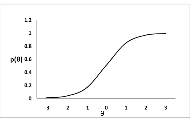
[image:27.612.110.434.339.540.2]the item parameters (a, b, and c parameter) as shown below.
Figure 1
The item characteristic curve for a dichotomous item
Lord’s chi-square statistic is given by
#B `4RBaRBbRBcd∑'<`4RBaRBbRBc, (7)
where
∑'<
is the inverse variance-covariance matrix for the differences in item parameter
estimates
0 0.2 0.4 0.6 0.8 1 1.2
-3 -2 -1 0 1 2 3
13
4RB 4:::ef: ghij" 4hf/k ghij (4 is the discrimination parameter)
aRB a:::ef: ghij" ahf/k ghij (a is the difficulty parameter)
bRB b:::ef: ghij" bhf/k ghij (b is the pseudo guessing parameter)
The distribution of Lord’s chi-square should be close to the chi-square
distribution with two degrees of freedom at 2PL model and that with three degrees of
freedom at 3PL model (Lord, 1980). Lord’s chi-square test is more useful with 2PL and
3PL models than with the 1PL model, since examining the difference between groups by
using only a one parameter model may provide inaccurate or insufficient results of DIF.
Type I error rate on DIF
In significance testing on DIF, the effective control of the Type I error rate has
been of interest. Many research findings have addressed the fact that the Type I error rate
is influenced by various conditions, and researchers have tried to control the Type I error
rate by setting factors differently. For instance, Uttaro and Millsap (1994) showed that
the MH method exhibited different Type I error rates for different test lengths: The result
for the 20 items test showed more inflation of Type I error rates than one for the 40 items.
Finch (2005) showed that the performance of the Simultaneous item bias test (SIBTEST)
is better in the two-parameter model than three -parameter model. Finch and French
(2007) showed that the performance of the Likelihood Ratio (IRTLR) test was low if the
sample size is small. The MH method performed poorly in the non- uniform DIF
The adjustment procedure in multiple significance testing can be an effective way
to control a Type I error rate. Although the probability of making a Type I error for each
significance test is set at some nominal α level, the overall α (the family-wise Type I
error rate, ]) across the entire set of significance tests can be considerably higher. The
family-wise Type I error rate is the probability of making at least one Type I error across
multiple significance tests. It is calculated as ] 1 " )1 " *f, where bis the number
of tests.
As said earlier, one issue in multiple significance testing is a higher chance of
committing a Type I error of identifying non-DIF items as DIF items. Common
approaches to control such an issue include the Bonferroni correction (Bonferroni, 1936),
the Holm’s procedure, and the Benjamini and Hochberg False Discovery Rate method
(Benjamini & Hochberg, 1995).
While the Bonferroni correction and the Holm’s procedure seek to control
family-wise Type I error rate, Benjamini and Hochberg (1995) controls expected false positive
discovery rates (FDR) by defining a sequential p-value procedure. The Benjamini and
Hochberg (BH) method for p-values 9<, ,9l follows as:
1. Rank order p-value of each item form the largest to the smallest
2. Remain the largest p-value
3. Multiply the second largest p-value by the total number of items in test and
15
4. Multiply the third largest p-value and divide by its rank as in Step 3 (corrected p-value = p-value*(n/(n-2)). If the corrected p-value < .05, it is significant.
continues until the smallest p-value is corrected.
The BH method has been adopted in the study of DIF (Steinberg, 2001; Thissen,
Steinberg, & Kuang, 2002; Williams, Jones, & Tukey, 1999). Williams, Jones, and Tukey
(1999) compared the BH method with the Bonferroni correction and showed the BH
method performed better. Steinberg (2001) also used the BH method with the likelihood
ratio procedure for the evaluation of DIF.
The Bonferroni correction is an adjustment to control family-wise Type I error
rate in multiple comparison procedures. If there are k hypotheses to be tested, each test should be conducted at significance level of nC , where k is the number of hypotheses (Holland & Cohenhaver, 1988).
The Bonferroni correction is a rough approximation, so it is conservative.
Perneger (1998) pointed out the problem of the Bonferroni adjustment. The main
weakness is that the Type I errors cannot be reduced without inflating Type II errors,
which is the probability of accepting the false negative, which is the mistake of failing to
reject a null hypothesis.
Holm (1979) presented an improved procedure that is more powerful than the
Bonferroni method (B. S. Holland & Copenhaver, 1987). The Holm’s procedure is very
similar to the Bonferroni, but it is known to be less conservative because the Holm’s
of the individual tests. The ordered p-value methods are strong for controlling a Type I
error rate, when the test statistics are independent (Shaffer, 1995).
The Holm’s procedure has two steps (Shaffer, 1995). The first step of the procedure is to order the k numbers of 9 values from the smallest to the largest and denote the ordered o9Bp by 9)<* 9)q*. Let )<*, , )q* be the corresponding
hypotheses. Suppose *
i is the smallest integer from 1 to k such that
9)Br* /)n " WrF 1* (8)
Then the Holm’s procedure rejects )<*, , )Br'<* and retains )Br*, ,
)q*. If 9)Br*is greater than /)n " WrF 1* for no integer Wr, then all k hypotheses are
rejected. Holm (1979) proves that this procedure guarantees that there is at most α chance
of rejecting at least one of the true hypotheses.
There are literature reviews on applying the Holm’s procedure in the areas of
clinical trials and biology. For example, Soulakova (2009) used the Holm’s procedure to
find a problem of identifying all effective and superior drug combinations. There is also
research on applying the Holm’s procedure to psychometrics for evaluating appropriate
curriculum based measurement of reading outcomes (Betts, Pickart & Heistad, 2009), but
none is found for the study of DIF so far.
Regarding the purpose of the dissertation, a literature review had been an account
of what has been studied on topics that were related with DIF studies. Relative articles
had been reviewed focusing on what methods were effective in a particular testing
17
procedures had been used to control the multiple significant testing issues in DIF studies,
and how DIF methods detect DIF items in terms of different criteria (until 2008). The list
18 CHAPTER 3
METHOD
Study Design
The research design consisted of two phases. The first phase conducted
significance testing of the four DIF methods; the performance of each DIF method was
then compared across all conditions. In order to answer the research questions,
significance testing of each DIF method was performed with a total of 16 conditions: 4
conditions of sample sizes × 2 conditions of test lengths × 2 conditions of group
difference (group mean difference (impact) and group standard deviation (SD)
difference). The second phase applied the Bonferroni correction, the Holm’s procedure,
and the BH method to the significance testing of each DIF method. A SAS program was
used to conduct the simulation studies and DIF analysis.
Conditions of Study
Data Generation
Using SAS program, the dichotomous scored data were generated for the
reference and the focal groups with a three-parameter IRT model. The ability of test
examinee was assumed to follow the standard normal distribution. First, the probability
of a correct response to an item was calculated based on pre-specified item parameters
from Oshima et al. (2006); the basis probability was generated at random from the
19
compared. If the basis probability was less than the calculated probability, the simulated
item response was scored as correct (1); otherwise, it was scored as incorrect (0).
Sample Size and Sample Size Ratio
Sample size is a core factor for detecting DIF items accurately. Although a small
sample size could cause a poor estimation, resulting in true DIF items not being detected
well, a large sample size could result in precise detection of true DIF items, although the
possibility exists that items with no or a very little DIF will be detected as if they are true
DIF items.
In most DIF research, the range of sample sizes is between 500 and 5,000 for both
equal and unequal sample sizes. This research chose total sample sizes of 1,000 and
2,000, etc. The ratio of the sample sizes between the focal group and the reference group
was also considered for non-parametric methods as existing research on DIF with
unequal sample sizes showed a greater tendency to detect flagged DIF items than one
with equal sample sizes (Kristjansson, Aylesworth, McDowell, & Zumbo, 2005).
However, the parametric method had one condition of the sample size (2,000) and an
equal ratio of sample sizes.
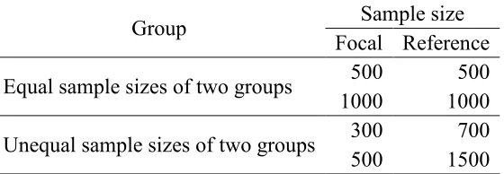
For the non-parametric method (Table 1), when the sample size was 1,000 and the
group sizes were the same, the size of each group was 500; when the group sizes were
different, the size of the reference group was 700 and that of the focal group was 300.
When the sample size was 2,000 and the group sizes were the same, the size of each
group was 1,000; when the group sizes were different, the size of the reference group was
Table 1
Sample size and sample size ratio of non- parametric methods
Group Sample size
Focal Reference
Equal sample sizes of two groups 500 500 1000 1000
Unequal sample sizes of two groups 300 700 500 1500
Test Length
This study chose test lengths of 20 items and 40 items. To date, much of the DIF
research has been conducted using a test length of between 20 and 40 items because
common assessments are constructed with fewer than 40 items. Raju et al. (1995)
selected 40 items in their simulation study. Roussos and Stout (1996) conducted their
simulation study with 25 items. In particular, 40 items has been chosen in many studies
(Jodoin & Gierl, 2001; Narayanan & H Swaminathan, 1994; Rogers & H Swaminathan,
1993).
Percent of DIF Level
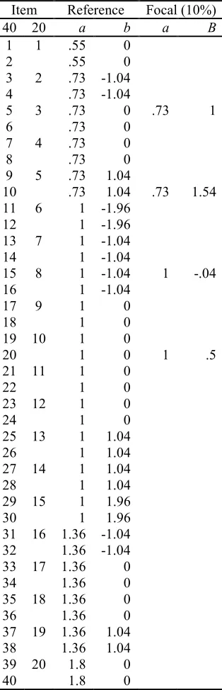
The setting of item parameters for data generation was identical to those in a
study by Raju et al. (1995) and Oshima et al. (2006). The condition of 10% DIF level was
investigated: All a, b and c item parameters were set to be the same for both reference and focal groups, except that two items (Item 3 and 8) in a 20 items test and four items
21
Table 2
Item parameters for the 40 items test and the 20 items test
Item Reference Focal (10%)
40 20 a b a B
1 1 .55 0
2 .55 0
3 2 .73 -1.04
4 .73 -1.04
5 3 .73 0 .73 1
6 .73 0
7 4 .73 0
8 .73 0
9 5 .73 1.04
10 .73 1.04 .73 1.54
11 6 1 -1.96
12 1 -1.96
13 7 1 -1.04
14 1 -1.04
15 8 1 -1.04 1 -.04
16 1 -1.04
17 9 1 0
18 1 0
19 10 1 0
20 1 0 1 .5
21 11 1 0
22 1 0
23 12 1 0
24 1 0
25 13 1 1.04
26 1 1.04
27 14 1 1.04
28 1 1.04
29 15 1 1.96
30 1 1.96
31 16 1.36 -1.04
32 1.36 -1.04
33 17 1.36 0
34 1.36 0
35 18 1.36 0
36 1.36 0
37 19 1.36 1.04
38 1.36 1.04
39 20 1.8 0
40 1.8 0
Group Difference
Two different conditions were set up. The first condition focused on the mean
difference between groups: the same mean between focal and reference groups versus
different means between the groups. The first component of the group means difference
was implemented by assuming that both reference and focal groups follow standard
normal distribution. The second component was implemented by assigning a lower mean
(by .2) to the focal group than to the reference group.
The second condition focused on the standard deviation (SD) difference between
the groups: no difference of SD between focal and reference groups versus different SD
between the groups. The first component of the group SD difference was implemented by
assuming that both reference and focal groups follow the standard normal distribution.
The second component was implemented by assigning a lower SD (by .2) to the focal
group than to the reference group (Penny & Johnson, 1999).
Replications
In order to ensure stable results, an appropriate number of replications were
needed. This study included 100 replications, because 100 times was the common
replication according to the publications of the National Council on Measurement in
23
Statistical DIF Methods for Simulation Studies
Four DIF methods were selected for this study: the MH method, the logistic
regression procedure, the DFIT method, and the Lord’s chi-square test. As an adjustment
of multiple significance testing, the Bonferroni correction, the Holm’s procedure, and the
BH method were applied.
DIF detection procedure for non-parametric methods
For each generated data set, the MH method and the logistic regression procedure
were used for DIF detection. Prior to DIF detection, ability matching for reference and
focal groups was performed by calculating the total scores (Zwick, J. R. Donoghue, &
Grima, 1993). Based on the total calculated score, matching ability was performed. This
study chose a form of thin matching used by Donoghue and Allen (1993). Thin matching
is based on using the total scores as the matching variable. The matching variable created
eight intervals. The total scores were then categorized into corresponding intervals in
order to match groups into equal intervals. After matching was completed, the statistics
of both the MH method and the logistic regression procedure were calculated for each of
replicated datasets.
DIF detection procedure for parametric methods
Several steps were needed in parametric DIF analyses. This study conducted two
stage-linking procedures. First, the generated data sets were calibrated using
BILOG-MG3 to obtain item parameter estimates. Second, item parameter estimates for reference
and focal groups were put on the common scale by determining linking coefficients
was used to determine cutoff scores and NCDIF values. The statistics of Lord’s
chi-square was also calculated using the Lord’s chi-chi-square test. Once DIF items were
detected, the second linking procedure was done by calculating linking coefficients again
with only non-DIF items. Using the new linking coefficients, refined statistics from the
25 CHAPTER 4
RESULTS
This study had two purposes. The first was an endeavor to investigate the degree
of the type I error rate with various factors. The second was to apply adjustment
approaches--specifically the Bonferroni correction, the Holm's procedure, and the BH
method--to a case of multiple significance tests on a DIF study. A total of 36 conditions
were simulated. In each condition, 100 replications were performed for each of the four
DIF methods, producing a total of 14,400 simulated data sets.
Although individual tests of each item were conducted at a Type I error rate of .05,
the overall Type I error rate and degree of power were questioned when multiple items
were tested concurrently (Hoffman & Recknor & Lee, 2008). The importance of
understanding the severity of an inflated Type I error rate has been discussed in other
studies (Lin &Rahman, 1998). In order to investigate the inflation of a Type I error rate,
Bradley’s (1978) liberal robustness criterion range of .025 to .075 was used. If a Type I
error rate for each DIF method was within this range, the Type I error rate was
considered well-controlled.
The test-wide Type I error rate for this study was calculated as follows. First, for
each replication, the occurrences of false positives out of all non-DIF items were counted.
Then, the proportion of these counts was calculated per replication, focusing on the
practical point of view how many items were falsely identified as DIF items in each test
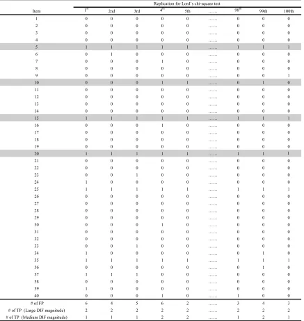
the false positives of the Lord’s chi-square test in a 40 items test; there are 4 DIF items
(Item 5, 10, 15, and 20) and 36 non-DIF items. The number of false positives is shown at
the bottom on the table: six in the 1st replication, four in the 2nd, and so on. The
proportion of false positives per replication was calculated out of 36 non-DIF items. That
is, the proportions of false positives were 6/36 in the 1st replication, 4/36 in the second,
and so on. The average of these proportions was .13; that is, the average of the test-wise
Type I error rate was .13. Therefore, on average, 13% of non-DIF items were falsely
identified as DIF items.
Type I error rate = <
27
Table 3
False positives and true positives for each item of Lord’s chi-square test in a 40 items test
* FP: False Positives, TP: True Positives * Highlighted rows indicated the DIF Items
1st 2nd 3rd 4th 5th …… 98th 99th 100th
1 0 0 0 0 0 …… 0 0 0
2 0 0 0 0 0 …… 0 0 0
3 0 0 0 0 0 …… 0 0 0
4 0 0 0 0 0 …… 0 0 0
5 1 1 1 1 1 …… 1 1 1
6 0 1 0 0 0 …… 0 0 0
7 0 0 0 1 0 …… 0 0 0
8 0 0 0 0 0 …… 0 0 0
9 0 0 0 0 0 …… 0 0 1
10 0 0 0 1 1 …… 0 1 0
11 0 0 0 0 0 …… 0 0 0
12 0 0 0 0 0 …… 0 0 0
13 0 0 0 0 0 …… 0 0 0
14 0 0 0 0 0 …… 0 0 0
15 1 1 1 1 1 …… 1 1 1
16 0 0 0 1 0 …… 0 0 0
17 0 0 0 0 0 …… 0 0 0
18 0 0 0 0 0 …… 0 0 0
19 0 0 0 0 0 …… 0 0 0
20 1 1 1 1 1 …… 1 1 1
21 0 0 0 0 0 …… 0 0 0
22 0 0 0 0 0 …… 0 0 0
23 0 0 1 0 0 …… 0 0 0
24 1 0 0 0 0 …… 0 0 0
25 1 1 1 1 1 …… 1 1 1
26 0 0 0 0 0 …… 0 0 0
27 0 0 0 0 0 …… 0 0 0
28 0 0 0 0 0 …… 0 0 0
29 0 0 0 0 0 …… 0 0 0
30 0 0 0 1 0 …… 0 0 0
31 0 0 0 0 0 …… 0 0 0
32 0 0 0 0 0 …… 0 0 0
33 0 0 1 0 0 …… 0 0 0
34 1 0 0 0 0 …… 0 1 0
35 1 1 1 1 1 …… 1 1 1
36 0 0 0 0 0 …… 0 1 0
37 1 1 1 0 0 …… 0 0 0
38 0 0 0 0 0 …… 0 0 0
39 1 0 0 0 0 …… 0 0 0
40 0 0 0 1 0 …… 1 0 0
# of FP 6 4 5 6 2 …… 3 4 3
# of TP (Large DIF magnitude) 2 2 2 2 2 …… 2 2 2
# of TP (Medium DIF magnitude) 1 1 1 2 2 …… 1 2 1
Item
The power rate in this study was also of interest. The investigation examined the
trend of power rate with two types of DIF magnitude that reflects the difference on item
parameters, since a power rate is affected by factors, such as the difference between two
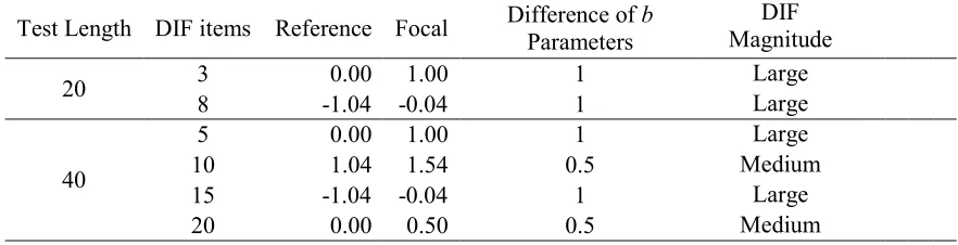
groups, sample size, etc. In this study, the difficulty (b) parameter value of each DIF item varied for the reference and focal groups, and I focused on the two magnitudes (large and
medium) of difference between the two groups. In the simulation, two items (Items 3 and
8) in the 20 items test and four items (Item 5, 10, 15, and 20) in the 40 items test were set
up as DIF items. The item difficulty (b) parameter values of these DIF items are shown in Table 4. For example, difficulty (b) parameters of Item 3 in a 20 items test are 0 and 1 for the reference and focal groups, respectively; their difference is 1. In the 40 items test,
differences of b parameters for Items 5 and 15 were all one, which was denoted as the large DIF magnitude; differences of b parameters for Items 10 and 20 were 0.5, which was denoted as the medium DIF magnitude. Therefore, the investigation of separated
[image:43.612.105.546.528.641.2]power rates by different DIF amount was needed in the 40 items test.
Table 4
Difference of b parameter for a 20 items test and a 40 items test
Test Length DIF items Reference Focal Difference of b Parameters
DIF Magnitude
20 3 0.00 1.00 1 Large
8 -1.04 -0.04 1 Large
40
5 0.00 1.00 1 Large
10 1.04 1.54 0.5 Medium
15 -1.04 -0.04 1 Large
29
The power rate was calculated in the similar way as the Type I error rate was
calculated. First, the proportion of true positives out of all DIF items with a specific DIF
magnitude was calculated for each replication. The power rate with a specific DIF
magnitude is the average of these proportions.
The highlighted rows in the Table 3 indicate DIF items. To calculate the power
rate with the large DIF magnitude, true positives out of two items (Items 5 and 15) in
each replication were counted first: two in the 1st replication, two in the 2nd, and so on.
Then, the proportion of true positives was calculated for each replication. The power rate
was the average of these proportions as shown below:
Power rate (large DIF magnitude) = <
<)2 2⁄ F 2 2⁄ F F 2 2⁄ * .99
Similarly, for the power rates with the medium DIF magnitude, true positives out of two
items (Items 10 and 20) were counted first: 1 in the 1st replication, 1 in the 2nd, and so
on. Then, the power rate was calculated as shown below:
Power rate (medium DIF magnitude) = <
<)1 2⁄ F 1 2⁄ F F 1 2⁄ * .55
All simulated false positives and true positives are presented in a tabular format in
Phase I
Research questions 1a and 1b listed previously addressed the effectiveness of
control for the Type I error rate for the four DIF methods under several testing conditions.
This study was also interested in comparing the Type I error rates of two non-parametric
methods (the MH method and the logistic regression procedure) with those of two
parametric methods (the DFIT method and the Lord’s chi-square test), to see which DIF
method performed better under specific conditions.
Comparing the Performance of Four DIF methods
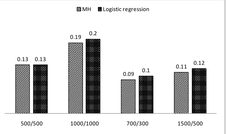
The results showed that the two non-parametric methods performed similarly
under all testing conditions considered in this study. For example, Figure 2 illustrates the
similarity between the MH method and the logistic regression procedure when Type I
error rates in the 20 items test were examined for different sample sizes. When the
sample sizes for reference and focal groups were both 500 (i.e., 500/500), the Type I
error rates for the MH method and logistic regression were both .13. For the sample size
of 1000/1000, the Type I error rates were .19 and .20 for the MH method and the logistic
regression, respectively. Similar interpretations apply to the sample sizes of 700/300 and
31
Figure 2
Type I error rate for non-parametric methods based on sample size with 20 items test
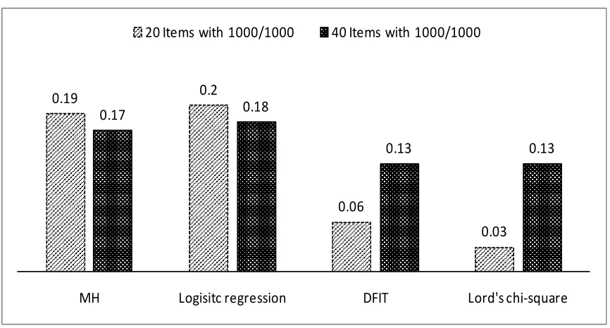
The two parametric methods, according to the results, also performed similarly
under all testing conditions considered in this paper except for the condition of different
test length. As shown in Figure 3, for the 20 items test, the Type I error rate of the DFIT
method was somewhat higher than that of the Lord’s chi-square test (.06 vs. .03). The
graphical comparison across the four DIF methods when the sample size is 1000/1000 is
presented in Figure 4. 0.13
0.19
0.09
0.11 0.13
0.2
0.1
0.12
500/500 1000/1000 700/300 1500/500
Figure 3
Type I error rate for parametric methods based on sample size 1000/1000
Figure 4
Type I error rates among four DIF methods with 1000/1000 sample size.
0.03
0.13
0.06
0.13
20 Item with 1000/1000 40 Item with 1000/1000 Lord's chi-square DFIT
0.19 0.2
0.06
0.03
0.17 0.18
0.13 0.13
MH Logisitc regression DFIT Lord's chi-square
[image:47.612.109.542.423.656.2]33
In sum, the four DIF methods--whether the method was non-parametric or
parametric--performed similarly for the 40 items test. However, with the 20 items test,
the Type I error rates of the non-parametric methods were higher than those of the
parametric methods (Figure 4). With further investigation, the effects of testing
conditions on Type I error rates of the four DIF methods were explained separately for
each testing condition.
The Effect of sample size conditions, sample size ratio, and test length
As previous research suggests (Bolt, 2000; Finch, 2005; Gotzmann & Boughton,
2004), both sample size and sample size ratio affected the Type I error rates for the DIF
methods. The MH method and the logistic regression procedure showed higher Type I
error rates for an equal ratio of sample sizes (500/500, 1000/1000) than for those of
unequal sample size ratios (700/300, 1500/500).
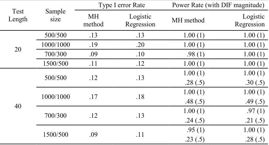
Table 5 shows Type I error rates and power rates of the MH method and the
logistic regression for the 20 items and 40 items tests with various sample sizes. For
example, for the 20 items test, the Type I error rate of the MH method was .13 when a
sample size was 500/500 for reference and focal groups. This rate was higher than the
Type I error rate of the same method for a sample size of 700/300 (.09). Additionally, the
Type I error rate of the MH method for the 20 items test in Table 5 was .19 for a sample
size of 1000/1000, which was higher than that the rate of the same method for a sample
size of 1500/500 (.11). For the logistic regression procedure for the 20 items test, the
for a sample size of 700/300. The Type I error rate with a sample size of 1000/1000
was .20, which was also higher than that (.12) for a sample size of 1500/500.
Table 5 also presents the power rate of both the MH method and logistic
regression procedure. In the 20 items test, the power rates were high for both
non-parametric methods since the DIF magnitudes of two both DIF items were large. In the
40 items test, the power rates with the large DIF magnitude were high across all
[image:49.612.108.547.356.592.2]conditions, but the power rates with medium DIF magnitude were very low.
Table 5
Type I error rate and power rate of non-parametric methods by test length and sample size
Test Length
Sample size
Type I error Rate Power Rate (with DIF magnitude)
MH method
Logistic
Regression MH method
Logistic Regression
20
500/500 .13 .13 1.00 (1) 1.00 (1)
1000/1000 .19 .20 1.00 (1) 1.00 (1)
700/300 .09 .10 .98 (1) 1.00 (1)
1500/500 .11 .12 1.00 (1) 1.00 (1)
40
500/500 .12 .13 1.00 (1) 1.00 (1)
.28 (.5) .30 (.5)
1000/1000 .17 .18 1.00 (1) 1.00 (1)
.48 (.5) .49 (.5)
700/300 .12 .13 1.00 (1) .97 (1)
.24 (.5) .21 (.5)
1500/500 .09 .11 .95 (1) 1.00 (1)
.23 (.5) .28 (.5)
35
The parametric methods--the DFIT method and the Lord’s chi-square test were
examined under only one sample size condition (1000/1000) since the DFIT method was
recommended for conditions of equal ratio and a sample size greater than 1000 similar to
SIBTEST (Gierl et al., 2004). The results are shown in Table 6. For the sample size of
1000/1000, the Type I error rates of the DFIT method and the Lord's chi-square test for
the 40 items test were .13 and .13, respectively; the Type I error rates for a 20 items test
for the two methods were .06 and .03.
The power rates of the parametric methods also showed similar pattern as the
non-parametric methods. The power rates were consistently high with the 20 items test.
The power rates with the 40 items test varied for different DIF magnitudes. When the
DIF magnitude was large, the power rates were high (above .99 across all conditions).
The power rates was low (.49 for DFIT method and .55 for the Lord’s chi-square test)
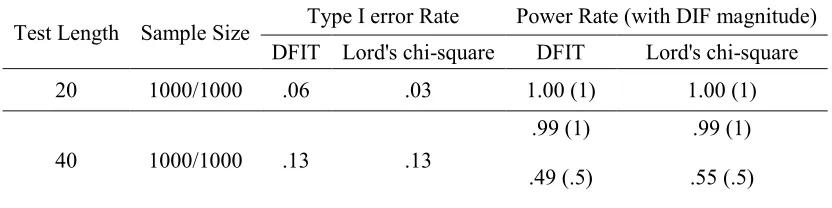
[image:50.612.106.522.507.611.2]with medium DIF magnitude.
Table 6
Type I error rate and power for parametric methods by test length and sample size
Test Length Sample Size Type I error Rate Power Rate (with DIF magnitude)
DFIT Lord's chi-square DFIT Lord's chi-square
20 1000/1000 .06 .03 1.00 (1) 1.00 (1)
40 1000/1000 .13 .13
.99 (1) .99 (1)
.49 (.5) .55 (.5)
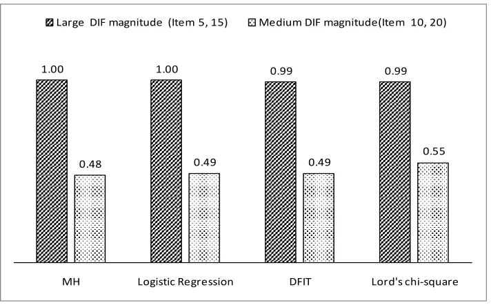
In summary, Figure 5 shows the overall patterns of the power rate for four DIF
methods for different DIF magnitude-large or medium. It shows a very strong and
consistent pattern. DIF items were detected with (almost) perfect accuracy with the large
[image:51.612.110.466.272.493.2]DIF magnitude.
Figure 5
The power rate of four DIF methods with 1000/1000 by different DIF magnitude
The Effect of Three Conditions for Group Difference
The performances of the four methods were first examined assuming the same
abilities between reference and focal groups—no group difference. The next analysis
addressed the effect of the assumption that the abilities of two groups had different
mean/standard deviation on the Type I error rates and power rates of the four methods.
As mentioned previously, two possible group difference conditions—group mean
difference and group SD difference—were set up. The analysis compared the
1.00 1.00 0.99 0.99
0.48 0.49 0.49
0.55
37
performances of the methods under each group difference condition with the
performances under no group difference condition. The results indicated that group SD
difference, but not group mean difference, highly affected the Type I error rates of three
methods: the MH method, the logistic regression procedure, and the Lord’s chi-square
test. The DIFT method was not affected much by either group difference conditions.
The results showed that the Type I error rates of the MH method under the group
mean difference condition were nearly the same as the rates under the no group
difference condition (Table 7). Similarly the power rates under the two conditions were
also very similar (Table 8). These results coincided with previous research: the trivial
effect of group mean difference (Sheppard, Han, Colarelli, Dai, & King, 2006).
The Type I error rates of the MH method under the group SD difference condition,
however, were different from the rates under the no group difference condition (Table 7);
the former rates were much higher than the latter rates. On the contrary, the power rates
under the group SD difference were lower than those under the no group difference
condition.
A similar pattern was found for the logistic regression procedure. The Type I rates
between the group mean difference condition and the no group difference condition were
similar. The power rates between the two conditions were also similar. However, the
Type I error rates were higher under the group SD difference condition than under the no
group difference condition; the power rates were lower under the former condition (Table
7 and Table 8).
The Type of I error rates of the Lord’s chi-square test between the group mean
However, the rate under the group SD difference condition for the 40 items test was
higher than its counterpart under the no group difference condition (Table 7). The power
rates of the Lord's chi-square test were similar for the two conditions: group mean
difference and no group difference conditions. On the other hand, the power rates under
the group SD difference condition were lower than those under the no group difference
condition (Table 8).
While the MH method, the logistic regression procedure, and the Lord’s
chi-square test were all affected by the group SD difference conditions discussed above, the
DFIT method was not affected much by any group difference conditions. In particular, in
the 20 items test, the Type I error rates were the same for all three conditions (.06) (Table
7). In the 40 items test, the Type I error rate under the group SD difference condition
were slightly higher than the rate under the no group difference condition. The power
rates under the group SD difference condition dropped slightly compared to those under
the no group difference condition. Therefore, the DFIT method showed the most stable
performance across the various group difference conditions.
In summary, the DFIT method seemed to be the most effective method for
controlling the Type I error rate, especially when the group SD difference existed because
it did not inflate the Type I error rate as much as the other methods. Across all conditions
of sample size, sample size ratio, test length, and group difference, the DFIT method
generally performed better than the other three methods1. Especially the DFIT method
performed very well under the condition of group SD difference compared to the other
1
39
methods. The finding presented here suggests that the group SD difference condition
inflates of the Type I error rate. Figure 6 and Figure 7 show the inflated Type I error rates,
under the group SD difference condition, of the four DIF methods in the 20 items test and
for the 40 items test, respectively.
The study results also suggest that high power rates were achieved with large DIF
magnitude items in general (Table 8). The power rates were lower when groups' SDs
were different than when there was no group difference or than when group means were
Table 7
Type I error rate for four DIF methods by group difference
Test Length Sample size Group Diff.
Type I error rate
MH method Logistic Regression DFIT Lord's chi-square
20 items test
500/500
No
.13 .13
1000/1000 .19 .20 .06 .03
700/300 .09 .10
1500/500 .11 .12
500/500
Mean
.11 .12
1000/1000 .16 .18 .06 .03
700/300 .10 .11
1500/500 .09 .10
500/500
SD
.23 .71
1000/1000 .36 .84 .06 .33
700/300 .20 .67
1500/500 .22 .63
40 items Test
500/500
No
.12 .13
1000/1000 .17 .18 .13 .13
700/300 .12 .13
1500/500 .09 .11
500/500
Mean
.11 .13
1000/1000 .16 .17 .13 .14
700/300 .11 .12
1500/500 .10 .11
500/500
SD
.16 .64
1000/1000 .25 .78
.15 .20
700/300 .16 .64
41
Table 8
The power rate for four DIF methods by group difference
Test Length Sample size Group Diff. Power Rate (With DIF magnitude)
MH method Logistic Regression DFIT Lord's chi-square
20 items test
500/500
No
1.00 (1) 1.00 (1) 1000/1000 1.00 (1) 1.00 (1) .95 (1) 1.00 (1)
700/300 .98 (1) 1.00 (1)
1500/500 1.00 (1) 1.00 (1) 500/500
Mean
1.00 (1) 1.00 (1) 1000/1000 1.00 (1) 1.00 (1) .96 (1) .99 (1)
700/300 1.00 (1) 1.00 (1)
1500/500 1.00 (1) 1.00 (1) 500/500
SD
.87 (1) .62 (1)
1000/1000 .97 (1) .66 (1) .84 (1) .48 (1) 700/300 .89 (1) .60 (1)
1500/500 .78 (1) .56 (1)
40 items Test
500/500
No
1.00 (1) 1.00 (1) .28 (.5) .30 (.5)
1000/1000 1.00 (1) 1.00 (1) .99 (1) .99 (1) .48 (.5) .49 (.5) .49 (.5) .55 (.5)
700/300 1.00 (1) 1.00 (1) 24 (.5) .28 (.5)
1500/500 .95 (1) .97 (1)
.23 (.5) .21 (.5)
500/500
Mean
1.00 (1) 1.00 (1) .33 (.5) .33 (.5)
1000/1000 1.00 (1) 1.00 (1) .97 (1) .99 (1) .49 (.5) .48 (.5) .35 (.5) .50 (.5)
700/300 1.00 (1) 1.00 (1) .29 (.5) .31 (.5)
1500/500 .97 (1) .98 (1)
.23 (.5) .21 (.5)
500/500
SD
.89 (1) .60 (1) .09 (.5) .66 (.5)
1000/1000 .98 (1) .62 (1) .81 (1) .58 (1) .16 (.5) .89 (.5) .53 (.5) .52 (.5)
700/300 .79 (1) .51 (1) .08 (.5) .74 (.5)
1500/500 .67 (1) .46 (1)
.11 (.5) .59 (.5)
Figure 6
Inflated Type I error rate with group SD difference for four DIF methods in a 20 items
test
Figure 7
Inflated Type I error rate with a group SD difference for four DIF methods in a 40 items test
0.36
0.84
0.06
0.33
MH Logisitc regression DFIT Lord's chi-square Group SD Difference (20 items)
0.25
0.78
0.15 0.20
MH Logisitc regression DFIT Lord's chi-square
[image:57.612.111.526.443.675.2]