www.hydrol-earth-syst-sci.net/15/405/2011/ doi:10.5194/hess-15-405-2011
© Author(s) 2011. CC Attribution 3.0 License.
Earth System
Sciences
A measure of watershed nonlinearity: interpreting a variable
instantaneous unit hydrograph model on two vastly different
sized watersheds
J. Y. Ding1,*
1Models and Consultative Services, Ontario Ministry of Natural Resources, 134 Heatherside Drive, Toronto, Ontario, M1W 1T9, Canada
*retired
Received: 30 August 2005 – Published in Hydrol. Earth Syst. Sci. Discuss.: 27 September 2005 Revised: 2 November 2010 – Accepted: 25 November 2010 – Published: 31 January 2011
Abstract. The linear unit hydrograph used in hydrologic de-sign analysis and flood forecasting is known as the trans-fer function and the kernel function in time series analysis and systems theory, respectively. This paper reviews the use of an input-dependent or variable kernel in a linear convo-lution integral as a quasi-nonlinear approach to unify non-linear overland flow, channel routing and catchment runoff processes. The conceptual model of a variable instanta-neous unit hydrograph (IUH) is characterized by a nonlin-ear storage-discharge relation,q=cNsN, where the storage exponentN is an index or degree of watershed nonlinearity, and the scale parametercis a discharge coefficient. When the causative rainfall excess intensity of a unit hydrograph is known, parametersNandccan be determined directly from its shape factor, which is the product of the unit peak ordinate and the time to peak, an application of the statistical method of moments in its simplest form. The 2-parameter variable IUH model is calibrated by the shape factor method and ver-ified by convolution integral using both the direct and in-verse Bakhmeteff varied-flow functions on two watersheds of vastly different sizes, each having a family of four or five unit hydrographs as reported by the well-known Minshall (1960) paper and the seldom-quoted Childs (1958) one, both located in the US. For an 11-hectare catchment near Edwardsville in southern Illinois, calibration for four moderate storms shows an average N value of 1.79, which is 7% higher than the theoretical value of 1.67 by Manning friction law, while the heaviest storm, which is three to six times larger than the next two events in terms of the peak discharge and runoff vol-ume, follows the Chezy law of 1.5. At the other end of scale, for the Naugatuck River at Thomaston in Connecticut
hav-Correspondence to: J. Y. Ding
(johnding [email protected])
ing a drainage area of 186.2 km2, the average calibrated N value of 2.28 varies from 1.92 for a minor flood to 2.68 for a hurricane-induced flood, all of which lie between the theoret-ical value of 1.67 for turbulent overland flow and that of 3.0 for laminar overland flow. Based on analytical results from the small Edwardsville catchment, the 2-parameter variable IUH model is found to be defined by a quadruplet of pa-rametersN,c, the storm duration or computational time step 1t, and the rainfall excess intensityi(0), and that it may be reduced to an 1-parameter one by defaulting the degree of nonlinearityN to 1.67 by Manning friction. For short, in-tense storms, the essence of the Childs – Minshall nonlinear unit hydrograph phenomenon is encapsulated in a peak flow equation having a single (scale) parameterc, and in which the impact of the rainfall excess intensity increases from the linear assumption by a power of 0.4. To illustrate key steps in generating the direct runoff hydrograph by convolution in-tegral, short examples are given.
1 Introduction
In a comprehensive survey of similarities and contrasts be-tween analyses of hydrologic elements and processes over a very large range of scales, Dooge (2005) makes a convincing case that progress in analysis has been made through simpli-fication of these complex processes. He advocates a strategy based on a rigorous analysis of simplified equations of
mo-tion (emphasis added). According to him, a wide range of
channels, and catchment runoff processes. Specifically, he reviews the work of Amorocho and Orlob (1961) on labora-tory experiments of overland flow, and of Minshall (1960) on unit hydrographs on a small experimental watershed.
The purpose of this paper is to present an additional ap-proach of simplification or approximation that the author has found useful, over his professional life of some 30 years, in unifying concepts behind these and other nonlinear pro-cesses in the context of rainfall excess – direct runoff mod-elling. In essence, this involves the use of an input-dependent or nonlinear kernel in a linear convolution integral, a relax-ation of the principle of superposition in linear systems. The concept of variable kernel or instantaneous unit hydrograph (IUH) will be reviewed, and the parameters reinterpreted. The classical example of the Minshall (1960) nonlinear unit hydrograph data on a small watershed in southern Illinois, the United States, will be analyzed using the variable IUH model to determine the degree of nonlinearity and scale pa-rameter. Another set of unit hydrograph data from an earlier study by Childs (1958) on a large Naugatuck River in Con-necticut, the United States, will be re-examined to determine its nonlinearity.
It is hoped this fresh look at two sets of some 50-year old unit hydrograph data from a nonlinear perspective will help identify areas for research by younger generations. Al-though the concept of nonlinear systems is not much diffi-cult to grasp than that of linear ones, it is found much harder to carry out numerical analysis for even a simple nonlinear system, such as the 2-parameter variable IUH model, charac-terized by a nonlinear storage-discharge relation,q=cNsN. Because of the presence of the exponentN, it is rather con-fusing, even to the author, to convert variables and parame-ters from one set of measurement units to another, short ex-amples will be given to illustrate key calculations.
2 Basic equations and assumptions for the overland flow
For flow over a plane subjected to a constant rate of rainfall excess, the continuity equation is expressed by:
ds
dt =i−q (1)
whereiis the inflow rate in mm/dt or mm h−1,qis the out-flow rate in mm/dt or mm h−1,s is the active or detention storage in mm, andtis time in h.
The equation of motion is approximated by a nonlinear storage-discharge relation:
q=cNsN (2)
where N is the storage exponent (dimensionless) known as a shape parameter, andc is the discharge coefficient in (mm/dt)1/N/mm or (mm h−1)1/N/mm, known as a scale pa-rameter. (Please note that parameterchaving the latter time
unit of hours now replaces the so-called standardizedChused extensively in the Discussion paper.)
For flow on a wide rectangular channel,N= 1.5 by Chezy friction law, and 1.67 by Manning (Horton, 1938; Ding, 1967a; Dooge, 2005). In the case of laminar overland flow, N= 3.0 (Horton, 1938; Izzard, 1946; Ding, 1967a). Note that Horton used the depth of flow instead of the volume of water in Eq. (2). The volume or storage is approximated by depth times the surface area. ParameterN has been proposed by Ding (1974) as an index or degree of nonlinearity for storage elements.
Equation (2) is known as a kinematic wave approximation to the equation of motion (Dooge, 2005). In the author’s view, Eq. (2) may be looked at more appropriately as a sim-plification of the Bernoulli energy equation, as it converts the potential energy (s)of a storage element into a kinetic energy (q)without loss. Therefore, some other form of the equation of motion will have to be specified to account for the flow acceleration.
In a review of overland flow data from laboratory exper-iments by Amorocho and Orlob (1961), Dooge (2005) ob-serves that if the laboratory system represents a wide rect-angular channel with Manning friction, then the characteris-tic time should be inversely proportional to the characterischaracteris-tic discharge to a power of 0.4. His analysis of their experimen-tal data shows a power of 0.3997, which is very close to the theoretical value.
For a laboratory watershed having a converging surface towards the outlet, Singh (1975), like Horton (1938) before him, used the local depth of flow in Eq. (2):
q=ahN (3)
wherehis the depth of flow at the outlet, andais a constant. Based on data from 210 experimental runs for 50 geo-metric configurations having varying physical characteristics collapsed into seven groups of similar surface characteristics, Singh (1975) found that parameterNis relatively stable, and parameterais extremely sensitive to rainfall input character-istics and surface composition, and that there exhibits a high correlation between the two. He fixed theN value at 1.5 by Chezy friction, which also led to a smaller variance of pa-rametera. For the 1-parameter kinematic wave model, he found the prediction error based on the hydrograph peak to be well below 25%.
The kinematic wave approximation, Eq. (2), can be modi-fied to simulate the hysteretic phenomenon by adding a term reflecting the rate of change in storage:
q=cNsN−c1 ds
dt (4)
wherec1 is a constant. Substituting ds/dt in Eq. (1) into Eq. (4):
s=1
c[c1i+(1−c1)q]
1/N (5)
WhenN=1, this reduces to the form of Muskingum model (Ding, 1967b, 1974).
The 3-parameter, nonlinear form of Muskingum model was evaluated by Gill (1978), Tung (1985) and Singh and Scarlatos (1987). Gill (1978) used a segmented-curve method to determine the three parameters on one test exam-ple and found an optimalN value of 1/2.347. Tung (1985) used four parameter optimization methods on the same test example and found theN values varying from 1/1.7012 to 1/2.3470. Note these fractional exponents are contrary to that of greater than unity as defined in connection with Eq. (2).
Singh and Scarlatos (1987) pre-set a moderately highN value of 2.0, and found that the model’s accuracy depends mainly on the scale parameterc, and unlike the linear case, the weighting factorc1is much less significant. They found that the use of a lowerN of 1.33 would improve the per-formance of the nonlinear model. A comparison by them with the linear case using four sets of inflow-outflow data shows that the nonlinear method is less accurate than its linear counterpart.
The Singh and Scarlatos (1987) findings are indicative of the stability problem associated with nonlinear analysis in which the impact of the inflow rate is amplified by the degree of system nonlinearity. It is noted that assessment on the ac-curacy of linear or nonlinear form of Muskingum model is complicated by the presence of local inflow along the river reach, which affects the accuracy of the outflow data used for calibration. The somewhat contradictory findings regarding the degree of nonlinearity by these investigators point to the need for verification by flume tests, similar to those for over-land flow in Sect. 2 above, in a hydraulic laboratory where the effects of local inflow can be eliminated or controlled.
Besides the looped storage-discharge relation, another characteristic of the Muskingum model is the occurrence of negative outflow rates at the beginning of the outflow hydro-graph (e.g. Chang et al., 1983). This problem can be fixed by imposing in Eq. (4) a non-negative condition forq, which, depending on the ratio of the storage to its rate of change, will define the size of computational time steps, generally larger.
In passing, the variable IUH model, which was origi-nally developed by Ding (1974) to simulate catchment runoff process, has been extended by Tsao (1981) for use as a flood routing model as well. This was also suggested by
Kundzewicz (1984) apparently unaware of his work which appeared in Chinese literature.
4 Similarity between catchment runoff and overland flow
The transformation of rainfall into runoff on small catch-ments, a building block of watershed models, is probably the most difficult problem to tackle in hydrology. A distinct fea-ture of the process is the existence of a time lag observed on most watersheds between a short, intense storm and the re-sultant hydrograph peak. The pair of continuity equation and the kinematic wave approximation (Eqs. 1 and 2) on their own, however, fails to model this characteristic time.
From a review of the Horton (1938) and Izzard (1946) ex-periments, Ding (1974) realized that the rising limbs of their overland flow hydrographs are essentially a summation, S-curve or S-hydrograph. This fact, apparently having been overlooked by previous investigators, provides a conceptual link to the catchment runoff process via a classical concept, which states that the ordinate of an instantaneous unit hydro-graph is the first derivative of an S-hydrohydro-graph normalized by the rainfall excess intensity. Mathematically, the relation between the two is expressed as follows:
u(t )= 1
i(0) dq(t )
dt (6)
where u(t ) is the IUH ordinate in h−1. Lesser known is the fact that the variableu(t ), representing the time rate of change in discharge, reflects the flow acceleration. Because of this, the IUH or, more precisely, the variable IUH which retains the rainfall excess intensity term, may be considered an alternate and simplified form of the equation of motion.
5 Catchment runoff process
For a special case of constant rainfall excess intensity over an indefinite period of time, i.e.i(t )=i(0)>0, Eq. (6) is a differential form of the linear convolution integral with an input-dependent or variable kernel:
q(t )= Z t
τ=0
i(t−τ )u[i(t−τ );τ]dτ (7) where u[i(0); t] is a nonlinear kernel associated with the causative rainfall excess intensity i(0). For convenience, u[i(0);t] will be abbreviated asu(t ), on the understanding that the IUH ordinate depends on the causative rainfall ex-cess intensity as well as the elapsed time.
Fig. 1. The Minshall family of unit hydrographs for the Ed-wardsville, Illinois, watershed, USA. (Reprinted with permission of ASCE.)
The use of an input-dependent kernel in the linear convo-lution integral was proposed by Amorocho (1967) to simu-late the systematic variation of the unit hydrographs observed by Minshall (1960) as shown in Fig. 1. The latter showed that on a 27.2-acre (11-hectare) experimental watershed near Edwardsville in southern Illinois, there exists not a single unit hydrograph, but a family of five, each dependent on its causative rainfall intensity. (This watershed will be referred to as the Edwardsville catchment.)
Similar phenomenon has been reported for medium-sized watersheds as well. For example, two years prior to Min-shall’s work, Childs (1958) presented an illuminating ex-ample of nonlinear runoff response for the 71.9 sq. mi. (186.2 km2)Naugatuck River at Thomaston in Connecticut. He showed, in Fig. 2, a family of four 3-hour unit hydro-graphs derived from flood records, in which as the flood peak discharge increases from a low of 3200 c.f.s. (91 m3s−1) to a high of 41 600 c.f.s. (1178 m3s−1 ), the latter caused by Hurricane Diane in August 1955, the unit hydrograph peak rate increases from approximately 3000 c.f.s. (85 m3s−1)to 7400 c.f.s. (211 m3s−1), and the peak time shortens from 9 h to 6.
[image:4.595.52.284.63.266.2]The work of Minshall (1960) has been cited by many studies as a classical case of nonlinear watershed response, some of which were cited previously by Ding (1974). Since then, other studies citing Minshall’s work include Overton and Meadows (1976), Chen and Singh (1986), Singh (1988), Robinson et al. (1995), Lee and Yen (2000), Cranmer et al. (2001), Sivapalan et al. (2002), Kokkonen et al. (2004), and Paik and Kumar (2004). By contrast, the work of Childs (1958) has rarely been cited, Ashfag and Webster (2000) be-ing a notable exception.
Fig. 2. The Childs family of unit hydrographs for the Naugatuck
River in Connecticut, USA. (Reprinted with permission of ASCE.)
6 Variable instantaneous unit hydrograph in catchment runoff process
Equation (7) is a linear or 1-dimensional convolution in-tegral having a variable kernel. It is of interest to note that a 2-dimensional extension having an additional vari-able kernel was proposed by Chen and Singh (1986). In keeping with the Dooge (2005) strategy of simplification, only the original 1-dimensional variable IUH model is re-viewed in this paper. Detailed derivation of the model and its properties can be found in the Ding (1974) paper. For his personal retrospective on the development of the model in the broader context of hydrologic modelling during the second half of the last century, including other technical details, the reader is invited to consult the 2-part consol-idated response (http://www.hydrol-earth-syst-sci-discuss. net/2/S1256/2006/hessd-2-S1256-2006.pdf).
6.1 Derivation of the variable IUH
The solution of Eqs. (1), (2) and (7) for a constanti(t )is a pair of parametric equations having a dummy variablev: u(t )=N cvN−1(1−vN)i1−1/N(0) (8) t= F (v,N )
Bakhmeteff function F(v,N)
0 0.5 1 1.5 2 2.5
Dummy variable v
0 0.1 0.2 0.3 0.4 0.5 0.6 0.7 0.8 0.9 1
N = 3.0
[image:5.595.51.284.63.224.2]N = 1.67 N = 1.001
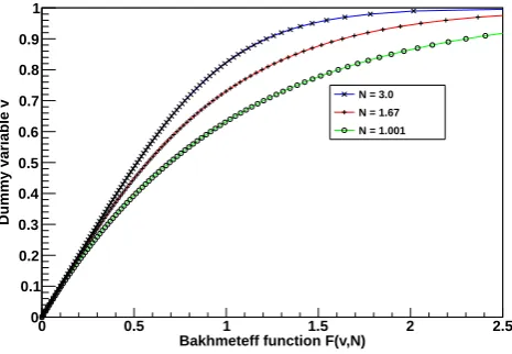
Fig. 3. The Bakhmeteff varied-flow function for three different
de-grees of watershed nonlinearity,N.N= 1.001 for nearly linear, 1.67
for moderately nonlinear, and 3.0 for highly nonlinear watersheds.
where F (v,N )=
Z v
v=0 dv
1−vN (10)
F (v,N ) is the well-known Bakhmeteff (1932) varied-flow function. Conceptually, v is not a dummy variable, but a normalized flow rate, [q(t )/i(0)]!/N.
Note in Eqs. (8) and (9), not only does the IUH ordinate vary directly, but also the elapsed time inversely, with the rainfall excess intensity to a power of (1–1/N ) so that the area under the IUH remains unity. The effect of parameterN on the IUH shape is complicated by the fact that it amplifies the impact of the rainfall excess intensity as well as having its own. The effect of parametercis straightforward, as it affects the IUH ordinate directly and elapsed time inversely. The fact that the elapsed time varies inversely with the intensity is found making calibration of the nonlinear model less straight forward than that of linear ones.
Substitutingu(t )in Eq. (8) into Eq. (7), the convolution integral becomes:
q(t )=N c
Z t
τ=0
vN−1(1−vN)i2−1/N(t−τ )dτ (11) Eqs. (9) and (11) constitute the 2-parameter, variable IUH model.
6.2 Bakhmeteff varied-flow function
To calculate the value of the varied-flow function, Bakhme-teff (1932) expands the integrand in Eq. (10) by the Taylor series and sums the successive higher-order terms:
F (v,N )= ∞ X
p=1
v(p−1)N+1
(p−1)N+1 (12)
Rp≤ vpN+1 pN+1·
1
1−vN (13)
whereRpis the residue of the series afterpnumber of terms. He sets the residual error at less than or equal to 0.0005.
As an example of calculation, forN= 1.67 by Manning friction and v= 0.473, the latter yields the IUH peak as shown in Sect. 6.7 below:
F (0.473,1.67)=0.473+(0.473) 2.67
2.67 +
(0.473)4.34 4.34 + (0.473)6.01
6.01 +
(0.473)7.68 7.68 +....
=0.473+0.051+0.009+0.002+0.000=0.535
Figure 3 shows the curves of the Bakhmeteff function for three different degrees of nonlinearity. Note the function and the time variablet are related linearly by Eq. (9). Thus the Bakhmeteff function tracks or traces the rising limb of an overland flow hydrograph.
6.3 Variable IUH peak characteristics
In Eq. (8), the peak ordinate of the IUH corresponds to the maximum value of the dummy-variable factor,vN−1(1–vN). Maximizing the factor yields:
v(tp)=
N−1
2N−1
1/N
(14) wheretpis time to the peak.
Substitutingv(tp)in Eq. (14) into Eqs. (8) and (9), the peak characteristics are expressed as follows:
u(tp)=Eci1−1/N(0) (15)
tp=tL=
F
ci1−1/N(0) (16)
where: E=N
2(N−1)1−1/N
(2N−1)2−1/N (17)
F=F[v(tp), N] (18)
Note these peak functions depend on the value ofNonly. In Eq. (16),tpis the time to IUH peak measured from the start of the rainfall-excess storm, and tL is the time to the peak from the mid-point of rainfall excess, the latter known as the basin lag or simply the lag. For the IUH in which1t approaches zero,tpandtLare identical.
The product ofu(tp)andtpdefines the shape of an IUH and is known as a shape factor. Model calibration by using the shape factor is a special, and the simplest, case of the method of moments in which only the time to peak and the peak ordinate are multiplied to calculate the statistical mo-ment. Product of Eqs. (15) and (16) yields:
6.4 Discretization of the variable instantaneous unit hydrograph model
The variable IUH model and its peak characteristics summa-rized above are mathematically derived treating the rainfall excess – direct runoff transformation as a continuous pro-cess. For application, the process will have to be sampled or discretized along the time axis.
Equations (11) and (9) in the continuous form are approx-imated by a discrete form as follows:
q(j )=N c
j X k=0
i2−1/N(j−k+1/2)vN−1(1−vN)1t (20)
j= F (v,N )
ci1−1/N(j−k+1/2)1t (21)
where indicesj andkare non-negative integers.
In comparison with the original formulation given by Ding (1974), there are two major differences worthy of noting. Firstly, in accordance with Fortran programming language convention, the index of a subscripted variable starts from 1, and not 0. This restriction is now removed. Secondly, a time-shift factor of (1t/2) now applies to the time index of the input variable,i(j 1t). This accounts for the inherent time-measurment lag that exists between the rainfall excess input, which is accumulated from (j −1)1ttoj 1thaving a midpoint at (j−1/2)1t, and the direct runoff output,q(j 1t), measured at the time instant or pointj 1t, even though both are recorded at the same time point,j 1t. Use of the time-shift factor synchronizes the rainfall excess series with the direct runoff one. See Fig. 2 for an illustration of the second point. Notationally, at time zero,i(0) =i(1) in this paper.
Note the IUH as represented by Eqs. (7) to (19) thus be-comes a1t-unit hydrograph (or1tUH for short). Since the midpoint of the rainfall excess, rather than the starting point, is more representative of the input variable,tLwill be used as a characteristic time. In a discrete form, the relation between the time to peak and the lag time is:
tp= 1t
2 +tL (22)
The IUH shape factor in Eq. (19) is now approximated by the 1tUH shape factor, which will be used to determine the de-gree of nonlinearity for both the Edwardsville and Naugatuck watersheds.
6.5 Conversion of the outflow rate
In applications of the variable IUH model, it has been found more intuitive to express both the variables and parameters in terms of the depth of water over the watershed. As a final step in hydrograph synthesis, the outflow rateqin mm h−1is converted to a new variableQhaving the familiar volumetric units of m3s−1. Let Abe the watershed area in km2, the relation between the two is:
Q=qA/3.6 (23)
6.6 Variable IUH equations for a unit pulse input For direct runoff hydrograph generated by a single block of rainfall excess and initially ignoring the time-shift factor, i.e.i(j−k+1/2)=i(0) when indicesj=k, andi(j−k+
1/2)= 0 otherwise, Eqs. (11) and (9) become:
q(j )=N ci2−1/N(0)vN−1(1−vN)1t (24) j= F (v,N )
ci1−1/N(0)1t (25)
At the time to peak, by making use of Eqs. (14), (17), (18) and (22), and putting back the time-shift factor of1t/2 into the time indexj, the above reduce to the following:
q(jp)=Eci2−1/N(0)1t (26)
jp=0.5+ F
ci1−1/N(0)1t (27)
wherejpis a multiple of1tdenoting the peak time. 6.7 Variable IUH by the Manning friction law
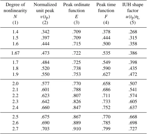
For N= 1.67 by Manning friction, the variable IUH shape factor is calculated in several steps: by Eq. (14), v(tp)= 0.473; Eq. (17),E= 0.722; Eq. (18),F= 0.535; and finally by Eq. (19),u(tp)tL= 0.386. Table 1 lists some other values of the IUH shape factor, which are extracted from a VUH Model manual (Ontario Ministry of Natural Resources, 1983).
Leti(0) =RE/1t whereREis the rainfall excess amount. Substituting the values of peak functions, E and F, into Eqs. (26) and (27) yields the following:
q(jp)=0.722c(RE/1t )1.41t (28) jp=0.5+
0.535 c(RE/1t )0.41t
(29) Equation (28) illustrates the relative effects on the peak dis-charge, of the rainfall excess intensity, and then equally the watershed discharge coefficient and the storm duration, if the Manning friction law holds on a watershed. Other things be-ing equal, given the same intensity, a longer duration storm would produce a higher peak discharge than a shorter one. A sensitivity analysis of the unit peak ordinate to change in parameterN,cor the rainfall excess intensityi(0) is given in Appendix A.
As a final step, the peak flow rateq(jp)in mm h−1is
con-verted by Eq. (23) to the peak dischargeQ(jp)in m3s−1as follows:
Table 1. Variable instantaneous unit hydrograph (IUH) shape factor.
Degree of Normalized Peak ordinate Peak time IUH shape nonlinearity unit peak function function factor
N v(tp) E F u(tp)tL
(1) (2) (3) (4) (5)
1.4 .342 .709 .378 .268 1.5 .397 .709 .444 .315 1.6 .444 .715 .500 .358
1.67 .473 .722 .535 .386
1.7 .484 .725 .549 .398 1.8 .520 .738 .590 .435 1.9 .550 .753 .627 .472
2.0 .577 .770 .658 .507 2.1 .601 .788 .686 .541 2.2 .623 .807 .711 .574 2.3 .642 .826 .733 .605 2.4 .660 .847 .752 .637
2.5 .675 .867 .770 .668 2.6 .690 .889 .785 .698 2.7 .703 .910 .799 .727
Source: Ontario Ministry of Natural Resources (1983) Col. (5):u(tp)tL= EF
6.8 Hydrograph generation by the direct and inverse Bakhmeteff function methods of convolution In hydrologic design analysis, one uses the convolution inte-gral as approximated by Eqs. (20) and (21). To generate the hydrograph ordinates at evenly-spaced time points, one com-putes the values of the Bakhmeteff function,F (v,N ),from Eq. (21), finds the corresponding values of dummy variable vby interpolation, and then computes the hydrograph ordi-nates by Eq. (20). This, we call for the purpose of this paper, the inverse Bakhmeteff function method of convolution, or the inverse method for short.
For short, intense storms, such as those reported by Min-shall (1960), one has an option of generating the hydrograph ordinates in high resolution or definition by computing the Bakhmeteff function directly. Given values of N, c,1t and i(0), one generates simultaneously the hydrograph ordinates and the elapsed times from Eqs. (20) and (21) by varying the dummy variablev from 0 to 0.99 at a v step of, say, 0.01. This we call the direct method of convolution.
6.9 Model calibration methodology
In the context of the variable IUH, the storage exponent N in Eq. (2) defines the degree of watershed nonlinearity. Ding (1998) conducted a survey of the variable IUH model applications in Ontario, Canada and in China (Collins and Moon Ltd., 1981; Tsao, 1981; Wisner et al., 1984; Chen and Singh, 1986) and reported that the calibratedN values
on watersheds ranging in size from one to 1900 km2 vary from 1.2 to 3.4.
As a form of simplification, Collins and Moon Ltd. (1981), in a calibration study in Ontario, Canada, fixed theN value at 1.5 according to Chezy friction, thus leaving only the scale parametercto be determined. For the normal range of storm events used in calibration, they found that the 1-parameter model does not suffer significant loss in its flexibility to fit observed hydrographs. For some 10 watersheds in south-western Ontario, they found that the scale parameter is in-versely proportional to watershed area to a power of 0.31, i.e. the larger the watershed, the smaller the discharge coefficient Given a pair of rainfall excess hyetograph and direct runoff hydrograph, the variable IUH model parameters can be simultaneously calibrated or optimized by the process of reversing the convolution integral (Eqs. 20 and 21), i.e. de-convolution. A parameter optimization procedure based on the method of differential corrections is given by Ding (1974). [Note: in Eq. (43) of the paper, the factor: vn0/ (1 –vn0)should readv n0lnv/ (1 –vn0).] However, this approach will not be followed because only the unit hy-drograph peak characteristics will be used for calibration.
Instead, an alternate approach called the variable IUH shape factor method will be used to determine or calibrate the shape parameterN, which in turn determines the scale parameterc. To verify the accuracy of calibrated parame-ters, hydrographs including the peak characteristics will be regenerated by applying both the direct and inverse Bakhme-teff function methods of convolution for comparison with ob-served one.
7 Analysis of the Minshall unit hydrograph data for the Edwardsville catchment
7.1 Shape parameter
The Minshall (1960) family of five unit hydrographs for the 11-hectare Edwardsville catchment is among the oft-cited examples of watershed nonlinearity. These storm events have a much wider range of rainfall values and provide an excellent data set for another closer look at the watershed nonlinearity.
Since Minshall (1960) provided data in the finished form of unit hydrographs, especially the peak rates and the time to peak, these lend themselves to the use of the IUH shape factor for calibration.
Table 2a. Unit hydrograph data for the Edwardsville catchment. Relation between rainfall intensity, unit hydrograph peak rate and time to
peak.
Runoff used in UH peak Time to
Rainfall producing UH computing UH ordinate peak
Storm Date Duration Amount Intensity Peak rate Amount
number 1t q(tp) RE u(tp) tp
min mm mm h−1 mm h−1 mm h−1 min
(1) (2) (3) (4) (5) (6) (7) (8) (9)
1 27 May 1938 14 28.19 120.81 60.45 16.76 3.61 12
2 2 Sep 1941 12 13.46 67.30 9.65 4.32 2.23 18
3 17 Apr 1941 13 10.67 49.25 6.35 3.56 1.78 20
4 22 Oct 1941 10 5.59 33.54 3.56 2.54 1.40 24
5 20 Jul 1948 17 6.86 24.21 6.35 5.33 1.19 30
[image:8.595.141.455.291.452.2]Source: adapted from Minshall (1960) and converted to metric units. Catchment area 11 hectare.
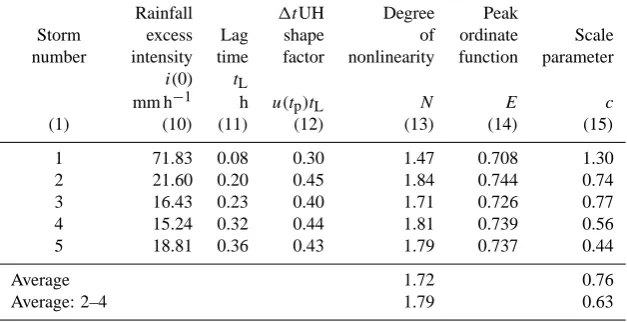
Table 2b. Unit hydrograph data for the Edwardsville catchment. Variable instantaneous unit hydrograph (IUH) model parameters.
Rainfall 1tUH Degree Peak
Storm excess Lag shape of ordinate Scale
number intensity time factor nonlinearity function parameter
i(0) tL
mm h−1 h u(tp)tL N E c
(1) (10) (11) (12) (13) (14) (15)
1 71.83 0.08 0.30 1.47 0.708 1.30
2 21.60 0.20 0.45 1.84 0.744 0.74
3 16.43 0.23 0.40 1.71 0.726 0.77
4 15.24 0.32 0.44 1.81 0.739 0.56
5 18.81 0.36 0.43 1.79 0.737 0.44
Average 1.72 0.76
Average: 2–4 1.79 0.63
Col. (15):cin (mm h−1)1/N/mm
arranged in the descending order of the rainfall intensity in Col. (5). Note the time to peak in Col. (9), when expressed in the multiple of the storm duration1tin Col. (3), is an integer of 1 to 2, i.e. the response time is very short.
Table 2b shows the calculations of the variable 1t UH model parameters. The rainfall excess intensity in Col. (10) is computed from the rainfall excess in Col. (7) and the storm duration in Col. (3). The range of rainfall excess intensity is found much narrower than that of rainfall intensity in Col. (5) and, in terms of the former, the lowest event is found out of order. In unit hydrograph analysis, data for the rainfall excess intensity, and not the rainfall intensity, are required, hence reference will be made to the former.
The lag time in Col. (11) is computed fromtpin Col. (9)
and1tin Col. (3). The IUH shape factor is approximated by the1tUH shape factor in Col. (12). According to Minshall (1960), periods of high rainfall intensity all occurred late in the storm for all five events. These imply that computed val-ues of the lag time may be too long, which may in turn cause
an over-estimation of parameterNvalues because, as can be seen from Table 1,N value increases as does the IUH shape factor. Because of absence of the observed data, their effects onNvalues will not be pursued. The degree of nonlinearity in Col. (13) is interpolated using Table 1 for a given value of the1tUH shape factor.
Table 2c. Unit hydrograph data for the Edwardsville catchment.
Regeneration of unit peak characteristics by the inverse Bakhmeteff function method of convolution.
Hydrograph peak Hydrograph peak time
Storm Peak Estimation Time to Estimation
number rate error peak error
q(tp) tp
mm h−1 % min min
(1) (16) (17) (18) (19)
1 34.93 −42.2 21 9
2 9.67 −0.2 18 0
3 6.36 0 20 0
4 3.55 0.3 25 1
5 6.09 −4.1 25 5
Prediction
1a 41.93 −30.6 21 9
1a,b 44.97 −25.6 23 11
1c 40.04 −33.8 21 9
1d 22.02 −63.6 21 9
abased on the averages of calibratedNandcvalues of storm nos. 2–5. bUsing a computational time step of1t/7, i.e. 2 min.
cBased on the maximumNandcvalues of storm nos. 2–5. cDoubling the averagedcvalue of storm nos. 2–5.
As mentioned in Sect. 2 above, in a review of the Amoro-cho and Orlob (1961) laboratory experimental data, Dooge (2005) concludes that the characteristic time is inversely pro-portional to the characteristic discharge to a power of 0.4. Note that the Dooge relation is of the same form as the Man-ning friction-based IUH peak time equation expressed by Eq. (29). It follows that for Amorocho and Orlob’s over-land flow plane, theN value is 1.67. This is in contrast to anNvalue of 1.5 for the Singh (1975) laboratory watershed having a converging surface.
7.2 Scale parameter
When parameter N has been determined, parameter ccan be determined from the IUH peak characteristics either by Eq. (15) or (16), and the results are shown in Table 2b and Fig. 4. The peak ordinate function in Col. (14) is computed by Eq. (17), and parametercin Col. (15) by Eq. (15). The c values vary from 0.44 to 1.30, with an average of 0.63 for four moderate storms. The calibratedc values have a much wider scatter than do theN values, with the highest cvalue, as well as the lowestN, associated with the largest event, storm no. 1. The lowestcvalue is associated with the 20 July 1948 event, storm no. 5, which had the longest du-ration of 17 min, compared to that of 10 to 14 min for the rest.
- 1 Rainfall excess intensity i(0) in mm h
0 10 20 30 40 50 60 70 80
V a ri a b le I U H M o d e l p a ra m e te rs 0 0.5 1 1.5 2 2.5 - 1 Rainfall excess intensity i(0) in mm h
0 10 20 30 40 50 60 70 80
V a ri a b le I U H M o d e l p a ra m e te rs 0 0.5 1 1.5 2 2.5 N c t ∆
t in h
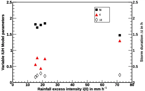
[image:9.595.52.287.119.309.2]∆ Storm duration 0 0.5 1 1.5 2 2.5
Fig. 4. Variations of the variable IUH model parameters with the
causative rainfall excess intensity as calibrated for five storms on the Edwardsville, Illinois, watershed.
7.3 Regeneration of unit hydrograph peak characteristics
The accuracy of parameters calibrated by the shape factor method in Sects. 7.1 and 7.2 above can be verified by ap-plying the convolution integral to regenerate hydrographs for comparison with the observed one.
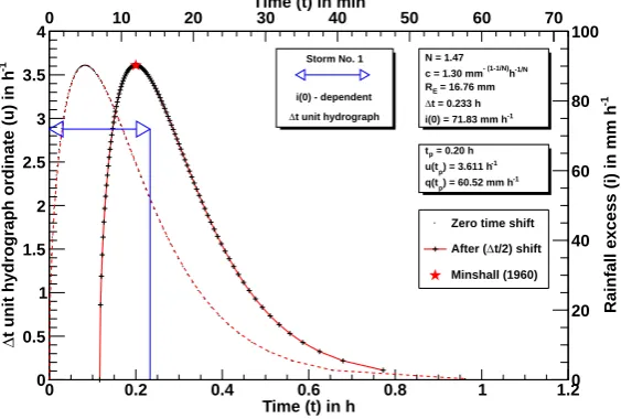
Based on the calibrated N and c values shown in Ta-ble 2b, hydrographs for each of the five events are regener-ated by convolution by, firstly the direct Bakhmeteff function method, and secondly the inverse method. Computations are done using a discrete form of the convolution integral with a variable IUH (Eqs. 20 and 21). In the computations, the time-shift factor of (1t/2) is ignored initially in the time index of the input variable, and the resultant hydrograph by convo-lution is then shifted forward in time by1t/2 to arrive at a regenerated hydrograph. The simulation results from using both the direct and inverse methods are shown, in Figs. 5a and b for storm no. 1, the largest event, and in Figs. 6a and b for the four moderate storms, storm nos. 2–5. In addition, results from the inverse method are tabulated in Table 2c.
For the largest event, storm no. 1, Fig. 5a shows that the direct method reproduces perfectly the peak characteristics, and Fig.5b shows that the inverse method under-captures the peak ordinate by about 42%. The inability of the inverse method to capture the peak rate may be, on the first glance, due to it’s being an atypical unit hydrograph, as explained in Sect. 7.1 above. Note that its time step (1t) of 14 min is larger than the time to peak (tp) of 12 min by 2 min or 17%, thus the1t unit hydrograph becoming an incomplete S-curve hydrograph, “incomplete” in the sense that it had not approached the state of equilibrium.
Time (t) in h
0 0.2 0.4 0.6 0.8 1 1.2
-1
t unit hydrograph ordinate (u) in h
∆
0 0.5 1 1.5 2 2.5 3 3.5 4
Time (t) in min
0 10 20 30 40 50 60 70
Storm No. 1
i(0) - dependent
t unit hydrograph
∆
N = 1.47 -1/N h - (1-1/N) c = 1.30 mm
= 16.76 mm E R
t = 0.233 h
∆
-1 i(0) = 71.83 mm h
= 0.20 h p t
-1 ) = 3.611 h p u(t
-1 ) = 60.52 mm h p q(t
-1
Rainfall excess (i) in mm h
0 20 40 60 80 100
Zero time shift
t/2) shift ∆ After (
[image:10.595.157.439.66.256.2]Minshall (1960)
Fig. 5a. Regeneration of the1tunit hydrograph by the direct Bakhmeteff function method of convolution for the largest storm, storm no. 1, on the Edwardsville, Illinois, watershed. For comparison, the peak characteristics reported by Minshall (1960) are shown as a red star.
Time (t) in h
0 0.2 0.4 0.6 0.8 1 1.2
-1
Direct runoff (q) in mm h
0 10 20 30 40 50 60 70
Time (t) in min
0 10 20 30 40 50 60 70
Storm No. 1
Regenerated
t hydrograph
∆
N = 1.47 -1/N h - (1-1/N) c = 1.30 mm
= 16.76 mm E R
t = 0.233 h
∆
-1 i(0) = 71.83 mm h
-1
Rainfall excess (i) in mm h
0 50 100
t hyd. - zero shift
∆
t/2) - shifted hyd.
∆
(
[image:10.595.155.441.308.499.2]Minshall (1960)
Fig. 5b. Same as Fig. 5b, except the1thydrograph is computed by the inverse Bakhmeteff function method of convolution.
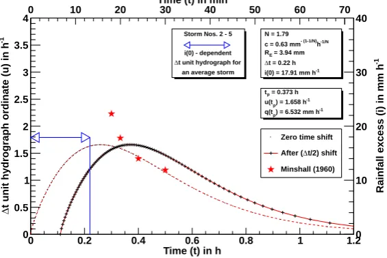
1t unit hydrographs for each of the four events, each of which reproduces perfectly its peak characteristics.) Simi-larly, Fig. 6b shows an average1t hydrograph produced by the inverse method of convolution. From results tabulated in Table 2c, the inverse method reproduces the moderate storms very well, having a maximum under-capturing rate of about 4%. Therefore, it may be concluded that for four moderate storms on the Edwardsville catchment, parameter values cal-ibrated by the shape factor method are correct.
7.4 Prediction of the extreme floods
One of the purposes of conducting model calibration on gauged watersheds is to obtain the best-fitted parameter
val-ues, and then apply these to predict or forecast hydrographs that would result from storms of greater magnitude.
Time (t) in h
0 0.2 0.4 0.6 0.8 1 1.2
-1
t unit hydrograph ordinate (u) in h
∆
0 0.5 1 1.5 2 2.5 3 3.5 4
Time (t) in min
0 10 20 30 40 50 60 70
Storm Nos. 2 - 5
i(0) - dependent t unit hydrograph for
∆
an average storm
N = 1.79 -1/N h - (1-1/N) c = 0.63 mm
= 3.94 mm E R
t = 0.22 h
∆
-1 i(0) = 17.91 mm h
= 0.373 h p t
-1 ) = 1.658 h p u(t
-1 ) = 6.532 mm h p q(t
-1
Rainfall excess (i) in mm h
0 10 20 30 40
Zero time shift
t/2) shift ∆ After (
[image:11.595.157.440.67.256.2]Minshall (1960)
Fig. 6a. Regeneration of the1tunit hydrograph by the direct Bakhmeteff function method of convolution for an average storm, using the averages of calibrated variable IUH model parameters for four moderate storms, storm nos. 2–5, on the Edwardsville, Illinois, watershed. For comparison, the peak characteristics reported by Minshall (1960) are shown as red stars.
Time (t) in h
0 0.2 0.4 0.6 0.8 1 1.2
-1
Direct runoff (q) in mm h
0 1 2 3 4 5 6 7 8 9 10
Time (t) in min
0 10 20 30 40 50 60 70
Storm Nos. 2 - 5
Regenerated t hydrograph for
∆
an average storm
N = 1.79 -1/N h - (1-1/N) c = 0.63 mm
= 3.94 mm E R
t = 0.22 h
∆
-1 i(0) = 17.91 mm h
-1
Rainfall excess (i) in mm h
0 10 20 30 40
t hyd. - zero shift
∆
t/2) - shifted hyd.
∆
(
Minshall (1960)
Fig. 6b. Same as Fig. 6b, except the1thydrograph is computed by the inverse Bakhmeteff function method of convolution.
from 1t/2 to 1t/(14×60), i.e. 7 min to 1 sec, the inverse method reduces the estimation errors to between−24% and
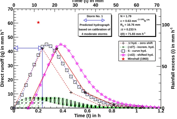
−26%, a fairly large amount but within a very narrow range. As an example, Fig. 7c shows the “predicted” hydrograph for the so-called storm 1bin Table 2c, which is computed using a time step of 2 min. Note the S-curve appears to represent the upper limit encompassing the predicted peak characteristics. In an attempt to improve the simulation accuracy of the peak ordinate, several other configurations were tested, but only two are included in Table 2c. Storm 1ctakes an “envelop curve” approach of using the maximums ofNandcvalues of the calibration group, and storm 1ddoubles the calibratedc value, the latter of which should have doubled the simulated peak ordinate by Eq. (20) alone. However, the simulation
results in Table 2c show that these two approaches worsen the accuracy of estimations by lowering it to about−34% and−64%, respectively.
[image:11.595.158.439.317.507.2]Time (t) in h
0 0.2 0.4 0.6 0.8 1 1.2
-1
t unit hydrograph ordinate (u) in h
∆
0 0.5 1 1.5 2 2.5 3 3.5 4
Time (t) in min
0 10 20 30 40 50 60 70
Storm No. 1
tUH
∆
i(0) - dependent
based on calibration of
4 moderate storms
N = 1.79 -1/N h - (1-1/N) c = 0.63 mm
= 16.76 mm E R
t = 0.233 h
∆
-1 i(0) = 71.83 mm h
= 0.259 h p t
-1 ) = 3.063 h p u(t
-1 ) = 51.32 mm h p q(t
-1
Rainfall excess (i) in mm h
0 20 40 60 80 100
Zero time shift
t/2) shift ∆ After (
[image:12.595.157.441.66.257.2]Minshall (1960)
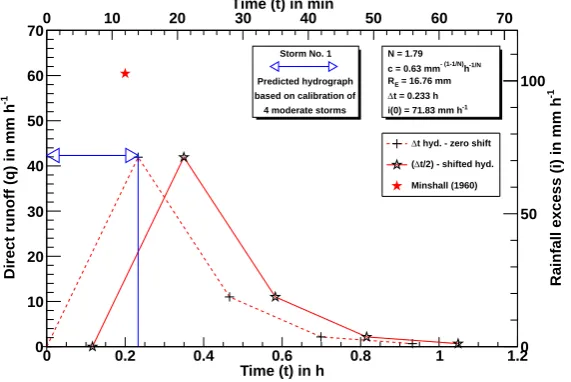
Fig. 7a. Prediction of the1tunit hydrograph for the largest storm, storm no. 1, on the Edwardsville, Illinois, watershed, using the calibrated variable IUH model parameters for four moderate storms, storm nos. 2–5, and by the direct Bakhmeteff function method of convolution. For comparison, the peak characteristics reported by Minshall (1960) are shown as a red star.
Time (t) in h
0 0.2 0.4 0.6 0.8 1 1.2
-1
Direct runoff (q) in mm h
0 10 20 30 40 50 60 70
Time (t) in min
0 10 20 30 40 50 60 70
Storm No. 1
Predicted hydrograph
based on calibration of
4 moderate storms
N = 1.79 -1/N h - (1-1/N) c = 0.63 mm
= 16.76 mm E R
t = 0.233 h
∆
-1 i(0) = 71.83 mm h
-1
Rainfall excess (i) in mm h
0 50 100
t hyd. - zero shift
∆
t/2) - shifted hyd.
∆
(
Minshall (1960)
Fig. 7b. Same as Fig. 7a, except the1thydrograph is computed using the inverse Bakhmeteff function method of convolution.
Note that to capture the peak ordinate of a hydrograph due to a single block of rainfall excess and pinpoint its time of occurrence, one can make use of the Manning friction-based peak equations given by Eqs. (28) or (30), and (29). For storm 1a, Eqs. (28) and (29) yield:
q(jp)=0.722×0.63×(16.76/0.233)1.4×0.233=42.16mm h−1
jp=0.5+0.535/[0.63×(16.76/0.233)0.4×0.233] =1.1591tor 16 min
which are comparable to those of 41.93 mm h−1and 21 min obtained by the inverse Bakhmeteff function method.
7.5 Size of the time step and its role in model application
All of those discussed in Sect. 7.4 above have profound im-plications for calibration, verification and application of lin-ear and nonlinlin-ear models alike, albeit in different ways, the variable IUH model included. (The linear models extrapo-late the peak magnitude of storm events in a straight line and fail to model the nonlinear Childs-Minshall phenomenon, the focus of the paper.)
[image:12.595.156.442.319.510.2]Time (t) in h
0 0.2 0.4 0.6 0.8 1 1.2
-1
Direct runoff (q) in mm h
0 10 20 30 40 50 60 70
Time (t) in min
0 10 20 30 40 50 60 70
Storm No. 1
Predicted hydrograph
based on calibration of
4 moderate storms
N = 1.79 -1/N h - (1-1/N) c = 0.63 mm
= 16.76 mm E R
t = 0.233 h
∆
-1 i(0) = 71.83 mm h
-1
Rainfall excess (i) in mm h
0 50 100
t hyd. - zero shift
∆
t/7) - increm. hyd.
∆
( S - curve hyd.
t/2) - shifted hyd.
∆
( Minshall (1960) N = 1.79
-1/N h - (1-1/N) c = 0.63 mm
= 16.76 mm E R
t = 0.233 h
∆
-1 i(0) = 71.83 mm h
t hyd. - zero shift
∆
t/7) - increm. hyd.
∆
( S - curve hyd.
t/2) - shifted hyd.
∆
[image:13.595.157.441.66.256.2]( Minshall (1960)
Fig. 7c. Same as Fig. 7b, superimposed by the incremental, composite or S-curve, and the time-shifted hydrographs using a computational
time step of1t/7, i.e. 2 min.
peak characteristics: the ordinate and the timing. The1tunit hydrograph generated by the direct method for a quadruplet of (N, c,1t andRE)or more intuitively, (N, c,1tandi(0)) as shown in Figs. 5a and 6a, provides both a window and a measuring stick, so to speak, to peek at and capture the mov-ing peak characteristics bemov-ing generated by the variable IUH model.
Imagine the time step1tas a stick or ruler of a fixed length and without decimal marks. As the length of the stick in-creases from near zero, the chance of its skipping the time to peak, thus the peak ordinate, becomes greater: the larger the time-step size, the greater the chance of missing the peak or-dinate. To capture the peak timetp, the time-step size1t, or its multiple, would have to be equal totp. But the search for a fixedtp, thus a fixed1t, proves elusive and futile, as the for-mer varies with, among others, the rainfall excess intensity as indicated by Eq. (16).
The role of the time-step size and its importance in hydro-logic modelling analysis have somewhat been overlooked, because one usually works with the hourly or even daily rain-fall and runoff data collected and published by government agencies. But given the Manning friction law which defines Nas 1.67,1tranks equally in importance withc, right after i(0), according to Eq. (28). Thus for the variable IUH model, N,c1tandi(0) form a quadruplet, among them inseparable from one another.
When the duration of a storm is less than the published time step of, say, 1 h, but is assumed to be so, this effectively under-reports the rainfall excess intensityi(0). To match the observed peak ordinate, according to Eq. (28), one has to increase thec value. (Or more directly, while the rainfall excess depthREremains the same, increasing1t should be accompanied by increasingcvalue so that the same peak or-dinate holds.)
Regarding the high c value of 1.30 calibrated from the largest event, storm no. 1, this should be considered as a result of curve-fitting. Since the scale parameter c is a discharge coefficient of the watershed storage as shown by Eq. (2):q=cNsN, heuristically one would expect thecvalue to be less than or equal to one. How could the water storage, active or detention one, contribute more than what it had to the outflow? Unless the storage operating like an “invisible hand” (to borrow Adam Smith’s famous phrase) in the rain-fall excess – direct runoff system was overloaded and over-taken by sheer force of the rainfall excess input under a big storm on a small catchment.
Similar cautionary note may sound to the use of highN values in hydrologic design analysis. In an inter-comparison study of three unit hydrograph models for six Ontario, Canada, watersheds, Wisner et al. (1982) obtained by curve fitting anN value of 1.9 for one watershed, and of 2.0 for another. For the latter, coupled with acvalue of 0.235 and a time step of 1 h, the variable IUH model generates unrealisti-cally high peak estimates for some design storm conditions. As noted in Sect. 6.1 above, parameterN amplifies the im-pact of the rainfall excess intensity by a power of (1–1/N )in unit hydrograph generation [and of (2–1/N ) in hydrograph one] as well as having its own on the peak ordinate, thus making the very high estimates when compared with those obtained by linear unit hydrograph models.
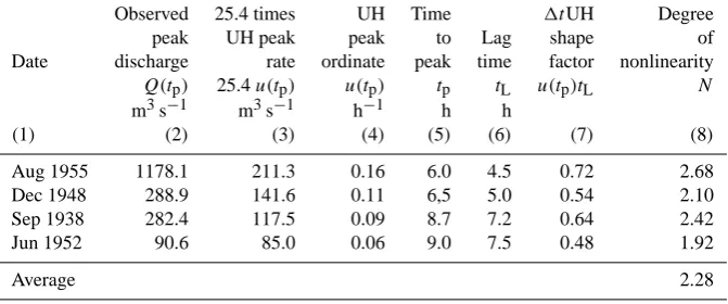
Table 3a. 3-hour unit hydrograph data for the Naugatuck River. Peak characteristics and calibration of the degree of nonlinearity.
Observed 25.4 times UH Time 1tUH Degree
peak UH peak peak to Lag shape of
Date discharge rate ordinate peak time factor nonlinearity
Q(tp) 25.4u(tp) u(tp) tp tL u(tp)tL N
m3s−1 m3s−1 h−1 h h
(1) (2) (3) (4) (5) (6) (7) (8)
Aug 1955 1178.1 211.3 0.16 6.0 4.5 0.72 2.68
Dec 1948 288.9 141.6 0.11 6,5 5.0 0.54 2.10
Sep 1938 282.4 117.5 0.09 8.7 7.2 0.64 2.42
Jun 1952 90.6 85.0 0.06 9.0 7.5 0.48 1.92
Average 2.28
Col. (3): 25.4 mm of runoff is the “unit” depth (1 inch) in the Childs unit hydrograph. Source: adapted from Childs (1958) and converted to metric units.
[image:14.595.95.501.320.448.2]Drainage areaA= 186.2 km2. Storm duration1t= 3 h
Table 3b. 3-hour unit hydrograph data for Naugatuck River. Calibration of the scale parameter and regeneration of peak characteristics by
the inverse Bakhmeteff function method of convolution.
Regenerated hydrograph
Peak Rainfall 68.58 times
ordinate excess Scale UH peak Peak Peak
Date function intensity parameter rate rate Error time Error
E i(0) c 68.58u(tp) q(tp) tp
mm h−1 (mm h−1)1/N/mm mm h−1 mm h−1 % h h
(1) (9) (10) (11) (12) (13) (14) (15) (16)
Aug 1955 0.906 22.86 0.025 10.99 9.26 −15.7 7.5 1.5
0.028 10.91 −0.7 4.5 −1.5
0.030 12.29 11.8 4.5 −1.5
Col. (12): 68.58 mm is the rainfall excess amount from the runoff rate of 0.9 in/h (or 22.86 mm h−1)for 3 h. ParameterN= 2.68
hydrograph ordinate and the elapsed time, any other com-binations of calibrated parameter values are shown to only slightly improve the simulation accuracy. But in practice, one does not have the luxury of using the direct method, due to the external constraint that the size of a time step is a fixed value, say 1 h, as pre-determined by rainfall and/or runoff measurements. Therefore one would have to take an approach similar to that of Wisner et al. (1982) to force the model to fit the observed peak characteristics, either the mag-nitude or the timing, or both, the latter seems rather unlikely. The calibrated parameter values so obtained are to be con-sidered product of curve fitting, rather than of physical rea-soning, if the degree of nonlinearityN is found significantly higher than 1.67 as dictated by Manning friction law.
8 Analysis of the Childs unit hydrograph data for the Naugatuck River
8.1 Shape parameter
As mentioned in Sect. 5 above, the Childs (1958) family of unit hydrographs for the Naugatuck River is an earlier but rarely cited example of watershed nonlinearity. Since he as-sociated the variation of the unit hydrographs with the ob-served (and thus effected) peak discharges, not the causative rainfall excess intensities, thus one key piece of data was missing for the calculation of parameterc.
Time (t) in h
0 2 4 6 8 10 12 14
-1
t unit hydrograph ordinate (u) in h
∆
0 0.05 0.1 0.15 0.2 0.25
August 1955
Hurricane Diane
Regenerated
t unit hydrograph
∆
N = 2.68 -1/N h - (1-1/N) c = 0.025 mm
= 68.58 mm E R
t = 3.0 h
∆
-1 i(0) = 22.86 mm h
= 6.0 h p t
-1 ) = 0.16 h p u(t
-1 ) = 11.05 mm h p q(t
-1
Rainfall excess (i) in mm h
0 5 10 15 20 25
Zero time shift
t/2) shift ∆ After (
[image:15.595.159.440.63.243.2]Childs (1958)
Fig. 8a. Regeneration of the 3-hour unit hydrograph for the Naugatuck River in Connecticut, by the direct Bakhmeteff function method of
convolution, for the Hurricane Diane in August, 1955. For comparison, the peak characteristics reported by Childs (1958) are shown as a red star.
Time (t) in h
0 2 4 6 8 10 12 14
-1
Direct runoff (q) in mm h
0 2 4 6 8 10 12
14 August 1955
Hurricane Diane
Regenerated
t hydrograph
∆
N = 2.68 -1/N h - (1-1/N) c = 0.025 mm
= 68.58 mm E R
t = 3.0 h
∆
-1 i(0) = 22.86 mm h
-1
Rainfall excess (i) in mm h
0 5 10 15 20 25
t hyd. - zero shift
∆
t/2) - shifted hyd.
∆
(
Childs (1958)
Fig. 8b. Same as Fig. 8a, except the1thydrograph is computed using the inverse Bakhmeteff function method of convolution.
descending order of the observed peak discharge in Col. (2). Column (3) shows the traditional “unit” hydrograph peak rates, i.e. for 1 inch (25.4 mm) of rainfall excess, which are read off the Childs graph in Fig. 2. The unit hydrograph peak ordinate in Col. (4) is computed from the peak rate in Col. (3) divided by the drainage area of 186.2 km2. Values for the time to peak in Col. (5) are also read off his graph. In terms of the storm duration of 3h, the time to peak is an integer of 2 to 3 in comparison with that of only 1 to 2 for the Ed-wardsville catchment. The1tUH shape factor and degree of nonlinearity for each of the events are computed in the same manner as described in Sect. 7.1 above for the Edwardsville. For the four 3-hour unit hydrographs, the calibrated N value varies from 1.92 to 2.68, with an average of 2.28. The smallestN value of 1.92 and the largest of 2.68 are associ-ated with the smallest and largest flood events, respectively.
They all lie between the theoretical value of 1.67 by Man-ning friction for turbulent overland flow, and that of 3.0 for laminar overland flow (Ding, 1967a).
When compared to the average nonlinearity of 1.79 for four moderate storms on the 11-hectare Edwardsville catch-ment, the larger Naugatuck River with a drainage area of 186.2 km2has a much higher nonlinearity of 2.28. Accord-ing to Eq. (2), between these two watersheds, the large river is more efficient in converting the flood storage into flood flow than the small catchment.
8.2 Scale parameter
[image:15.595.156.438.304.482.2]For the August 1995 Hurricane Diane, Childs (1958) re-ported that the computed peak discharge of 41 600 c.f.s. was equivalent to a rate of runoff of 0.9 inches per hour from the entire drainage area of 72 sq. mi., and that the rate of rainfall probably did not greatly exceed a basin-wide aver-age of 1 inch per hour, thus the Naugatuck River becoming a proverbial “tin-roof ” (in Childs’ word) under extreme flood conditions.
Based on his estimated rainfall excess intensity of 0.9 inches per hour (or 22.86 mm h−1), parametercis calcu-lated by the same shape factor method, which gives acvalue of 0.025 as shown in Table 3b. This is very much smaller than the average cvalue of 0.63 for four moderate storms on the Edwardsville catchment, i.e. the larger the watershed size, the smaller the discharge coefficient.
8.3 Regeneration of unit hydrograph peak characteristics
Based on calibratedN andcvalues shown in Tables 3a and b, the 1t unit hydrograph and1t hydrograph for the Au-gust 1955 flood event are regenerated using both the direct and inverse Bakhmeteff function methods of convolution and shown in Figs. 8a and b, respectively. Results from the latter are also shown in Table 3b. For the Naugatuck River with a computational time step of 3h, the direct method again re-produces perfectly the peak characteristics, but the inverse method under-captures the peak ordinate by about 16%. In-creasing the calibratedcvalue from 0.025 to 0.028, or about 10%, would reduce the under-capturing rate to about 1%. Again, same caution applies about the use of a higher N value and the relative large1t relative to the time to peak as described in Sects. 7.4 and 7.5 above.
9 Summary and conclusions
The author has described conceptual linkages between non-linear overland flow, channel routing and catchment runoff processes through the use of an input-dependent kernel or variable IUH. A 2-parameter variable IUH model has been applied to two watersheds of vastly different sizes. The cali-bration for the Edwardsville and Naugatuck watersheds both is carried out using their unit hydrograph shape factor, be-cause of the availability of the unit hydrograph data in a finished form. Based on analysis of these well-documented storm events, but mainly on one small catchment, a number of conclusions regarding the model are summarized below.
General
a. In the context of rainfall excess – direct runoff mod-elling, the variable IUH model having a shape param-eterN and a scale parametercis one of the simplest
nonlinear models reported in literature. These two pa-rameters plus the unit storm data: the duration1t, and either the rainfall excess depthREor rainfall excess in-tensityi(0), constitute a quadruplet that completely de-fines the model. Changing one of its parts, such as1t, would affect the others, as they are related, for example, by Eqs. (28) and (29) for a Manning friction law – based system.
b. There are two ways of computing the convolution in-tegral representing the variable IUH model. The di-rect Bakhmeteff function method, which generates the unit hydrograph in high definition, reproduces perfectly the peak characteristics resulting from short, intense storms. By contrast, the inverse Bakhmeteff function method, which generates the hydrograph ordinates at evenly-spaced time points, always under-captures the peak ordinates because of the non-zero size of the com-putational time step 1t; the larger the size of a time step, the greater the magnitude of under-capturing.
Shape parameter
c. The Minshall (1960) unit hydrograph data for the 11-hectare Edwardsville catchment show mixed results. For moderate storms, the degree of nonlinearity aver-ages 1.79, or 7% higher than the theoretical value of 1.67 by Manning friction. For the largest event, which has an atypical unit hydrograph in that it peaked prior to the end of the storm, and is an outlier in terms of the peak discharge, it has anN value of 1.47, close to the theoretical value of 1.5 by Chezy friction.
d. The Childs (1958) unit hydrograph data for the Nau-gatuck River having a drainage area of 186.2 km2 indi-cate a highly nonlinear river basin withN values rang-ing from 1.92 to 2.68 with an average of 2.28. These lie between the theoretical value of 1.67 for turbulent overland flow by Manning friction, and that of 3.0 for laminar overland flow.
Scale parameter
e. The larger Naugatuck River has acvalue of 0.025 cal-ibrated from a hurricane-induced flood, and the smaller Edwardsville catchment has an average calibrated value of 0.63 for four moderate storms. Given similarN val-ues, the larger the watershed size, the smaller the dis-charge coefficient.
Computational time step
computational time step. The use of a single time step of the full storm duration is next to the best available to ap-proximate the peak magnitude by the inverse Bakhme-teff function method of convolution. Decreasing the size of time steps beyond a factor of 2 does not signifi-cantly improve simulation accuracy.
Interaction of parameters and the time step
g. ParametersN andc are calibrated by the unit hydro-graph shape factor method, and verified by convolu-tion. For the Edwardsville catchment having storm du-rations in the order of 10 min, both the direct and in-verse Bakhmeteff function methods give similar peak rates for moderate events. For the Naugatuck River hav-ing a storm duration of 3h for the hurricane-induced August 1955 flood, the inverse method using the cali-brated parameters under-captures the peak discharge by about 16%.
h. The model parameters are applicable to the size of time step for which they are calibrated.
i. To calculate hydrograph peak characteristics produced by a block of uniform rainfall excess, the IUH peak equations (Eqs. 29 and 30) are available for such a pur-pose. This pair of Manning friction-based equations, having a single (scale) parameterc, crystallizes and cap-sulizes at once the essence of nonlinear unit hydrograph phenomenon explored by Childs (1958) and Minshall (1960), modelled by, among others, Amorocho (1967), Overton and Meadows (1976) and the author (Ding, 1974), the latter’s work further extended by Chen and Singh (1986).
j. For hydrologic design purposes, the instantaneous unit hydrograph and the S-curve hydrograph approaches ap-pear to encompass the design hydrograph shape, includ-ing the peak characteristics, resultinclud-ing from a uniform rainfall excess series.
Application to ungauged basins
k. For small ungauged watersheds, by defaulting the de-gree of nonlinearityN to the theoretical value of either 1.67 by Manning friction (or 1.5 by Chezy), the variable IUH model reduces to a single parameter one, leaving only the scale parametercto be determined. Parameter chas a very appealing property in that the IUH peak or-dinate varies directly and the peak time inversely with it. The scale parameterc, when calibrated for more wa-tersheds under a wide range of storm sizes, may be re-gionalized to provide guidance for prediction or design purposes on ungauged basins.
Appendix A
Sensitivity of the unit peak ordinate
Equations (8) and (9) show that the unit hydrograph ordi-nates,u(tp)included, vary linearly, and the elapsed times in-versely, with parameterc, but they vary with parameter N in a more complicated manner. The latter is caused by its presence in the power of the rainfall-excess-intensity term, i1−1/N(0), which amplifies the impact of the intensity by a power of (1–1/N )on the peak characteristics. Since param-eterN has its own impact, intuitively, the unit peak ordinate is expected to vary more withN thanc.
Mathematically, the sensitivity of u(tp) to change in ei-ther N or c can be expressed by the partial derivatives of u(tp)=Eci1−1/N(0)in Eq. (15) with respective to each of the parameters as given below:
∂[u(tp)] ∂N =ci
1−1/N(0)∂E
∂N+
Eci1−1/N(0)lni(0)
N2 =
(1 E
∂E ∂N +
lni(0)
N2 )u(tp) (A1)
∂[u(tp)] ∂c =Ei
1−1/N(0)=u(tp)
c (A2)
whereE is the peak ordinate function given previously by Eq. (17):
E=N
2(N−1)1−1/N
(2N−1)2−1/N
The derivative of functionEwith respective toNas required by Eq. (A1) is rather complicated, but can be simplified by making use of the expression forEitself:
∂E ∂N =
N+ln[(N−1)/(2N−1)]
N2 E (A3)
Equation (A1) can then be rewritten as follows: ∂[u(tp)]
∂N =
lni(0)+N+ln[(N−1)/(2N−1)]
N2 u(tp) (A4)
Note that on the right-hand side of Eq. (A4), the numerator excludingu(tp)can be negative in value. Therefore compar-isons should be based on its absolute value.
Equation (A2) shows that the sensitivity ofu(tp)to change incis itself the ratio ofu(tp)toc, i.e.u(tp) varies linearly withcwith a gradient ofEi1−1/N(0), butEitself is a func-tion ofN. Eq. (A1) shows a more complicated relation be-tweenu(tp)andN.
The relative sensitivity of u(tp) to changes in N andc depends on their relative magnitude. If one were to de-fault parameterN to some constant,N should have less ex-planatory power thancin the variance of the peak ordinate. Statistically,
∂[u(tp)] ∂N
≤∂[u(tp)]