Seismogeodetic Imaging of Active Crustal Faulting

(1)

Thesis by

Asaf Inbal

In Partial Fulfillment of the Requirements for the degree of

Doctor of Philosophy

CALIFORNIA INSTITUTE OF TECHNOLOGY

Pasadena, California

2017

(2)

Asaf Inbal

ORCID: 0000-0001-8848-7279

(3)

ACKNOWLEDGEMENTS

I would like to acknowledge the immense support I have received from my mentors

Jean-Paul Ampuero, Rob Clayton, and Jean-Philippe Avouac throughout my studies

at Caltech. J.-P. Ampuero’s rigorous approach and persistence, broad knowledge, scientific intuition and precision were a source of inspiration over these years. His

guidance have shaped the manner in which I conduct scientific research. R. Clayton

introduced me into to the subject of dense seismic array seismology. I was

fortu-nate to learn from his rich experience and knowledge in the field of seismic wave

propagation and migration, big data processing, regional tectonophysics, seismic

field operations and more. His deep enthusiasm and joy of making scientific

dis-coveries effectively acted as a powerful engine advancing my research. J.-P. Avouac

introduced me into the field of geodetical imaging and finite fault inversions. His

ample experience and deep understanding of tectonic processes on multiple

spatio-temporal scales, the mechanics of faulting and friction helped in clarifying many concepts associated with the joint strain and earthquake approach. Alon Ziv

pro-vided important insights regarding the joint strain and seismicity analysis, which

significantly contributed to the development of this technique. His timely and

valu-able advice helped me make difficult decisions at important junctions along the way.

Discussions with Hiroo Kanamori and Mark Simons raised important issues and

questions touching the foundations of seismological research, which helped sharpen

my own scientific perspective. Dan Hollis provided us with the Long-Beach dense

array data set, and was also helpful in conduction field work during our Lost Hills

deployment. I would like to thank my wife Cecilia Iribarren for creating the stable and unshakable ground of true friendship, and to my parents Dodik and Shoshi

Inbal, and my brother Boaz Inbal, who gave me the courage and strength to peruse

(4)

(5)

ABSTRACT

Monitoring microseismicity is important for illuminating active faults and for

im-proving our understanding earthquake physics. These tasks are difficult in urban

areas where the SNR is poor, and the level of background seismicity is low. One example is the Newport-Inglewood fault (NIFZ), an active fault that transverses the

city of Long-Beach (LB). The catalog magnitude of completeness within this area is

M=2, about one order of magnitude larger than along other, less instrumented faults

in southern California. Since earthquakes obey a power-law distribution according

to which for each unit drop in magnitude the number of events increases by a tenfold,

reducing the magnitude of completeness along the NIFZ will significantly decrease

the time needed for effective monitoring. The LB and Rosecrans experiments

pro-vides a unique opportunity for studying seismicity along the NIFZ. These two array

contain thousands of vertical geophones deployed for several-months periods along

the NIFZ for exploration purposes. The array recordings are dominated by noise sources such as the local airport, highways, and pumping in the nearby oil fields.

We utilize array processing techniques to enhance the SNR. We downward continue

the recorded wave field to a depth of a few kilometers, which allows us to detect

signals whose amplitude is a few percent of the average surface noise. The migrated

wave field is back-projected onto a volume beneath the arrays to search for seismic

events. The new catalog illuminates the fault structure beneath LB, and allows us

to study the depth-dependent transition in earthquake scaling properties.

Deep aseismic transients carry valuable information on the physical conditions

that prevail at the roots of seismic faults. However, due the limited sensitivity of

geodetic networks, details of the spatiotemporal evolution of such transients are

not well resolved. To address this problem, we have developed a new technique to

jointly infer the distribution of aseismic slip from seismicity and strain data. Our

approach relies on Dieterich (1994)’s aftershock model to map observed changes

in seismicity rates into stress changes. We apply this technique to study a

three-month long transient slip event on the Anza segment of the San Jacinto Fault (SJF),

triggered by the remote Mw7.2, 2010 El Mayor-Cucapah (EMC) mainshock.

The EMC sequence in Anza initiated with ten days of rapid (≈100 times the

long-term slip rate), deep (12-17 km) slip, which migrated along the SJF strike. During

the following 80 days afterslip remained stationary, thus significantly stressing a

(6)

cumulative moment due to afterslip induced by the later mainshock is about 10 times larger than the moment corresponding to the mainshock and its aftershocks. Similar

to sequences of large earthquakes rupturing fault gaps, afterslip generated by the two

mainshocks is spatially complementary. One interpretation is that the stress field

due to afterslip early in the sequence determined the spatial extent of the late slip

episode. Alternatively, the spatial distribution is the result of strong heterogeneity

of frictional properties within the transition zone. Our preferred model suggests

that Anza seismicity is primarily induced due to stress transfer from an aseismically

slipping principal fault to adjacent subsidiary faults, and that the importance of

(7)

PUBLISHED CONTENT AND CONTRIBUTIONS

Inbal, A., J.-P. Ampuero, and J.-P. Avouac. “Locally and remotely triggered afterslip on the central San Jacinto Fault near Anza, CA, from joint inversion of strain and earthquake data”. In:J. Geophys. Res.In review. A.I. wrote and implemented the software used to process the strain and aftershock data, and perform the inversion ; generated the figures; analyzed the results; and wrote the manuscript.

Inbal, A., J.-P. Ampuero, and R.W. Clayton. “Localized deformation in the upper mantle revealed by dense seismic arrays”. In: Science. In press. A.I. wrote and implemented the software used to process the LB data set ; generated the figures; analyzed the results; and wrote the manuscript.

(8)

LIST OF ILLUSTRATIONS

Number Page

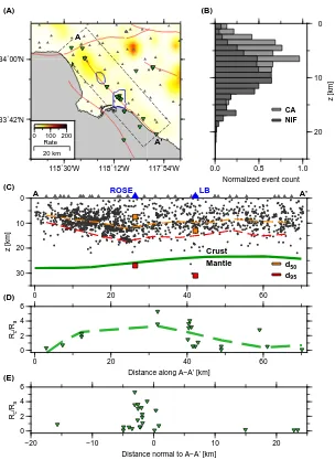
2.1 The spatial distribution of seismicity that occurred between

1980-2011 and was recorded by the Southern California Seismic

Califor-nia (SCSN), and Helium ratios (3He/4He) in the LA basin, which were measured and corrected for air contamination by Boles et al. (2015). (A) The earthquake density as a function of location. We

used the color bar labeled "Rate" to indicate the spatially smoothed

number of events over a 30-year period, binned in 9 km2 squares. The location of Helium measurements, seismic stations, and dense

seismic arrays are denoted by green inverted triangles, gray

trian-gles, and blue polygons, respectively. We indicated the region from

which we extracted the earthquakes we used in panels B and C by

the dashed curve, and the surface trace of active faults by red curves.

(B) The SCSN catalog seismicity depth distribution along the NIFZ

and in southern California. (C) The depths of NIFZ seismicity and

the Moho as function of location along line A-A’ in panel A. The

Moho is indicated by the green curve. The depths above which 50% and 95% of the earthquakes occur in the SCSN and back-projection

derived catalogs are indicated by the orange and red dashed curves

and squares, respectively. (D) The Helium ratios within the area

enclosed by the dashed polygon in panel A as a function of distance

along A-A’. The polynomial best fit to the observations is indicated

by the dashed curve. (E) The Helium ratios as a function of distance

(10)

2.2 Amplitude as a function of time for traces containing aMw =0.4, and back-projected stack amplitude as a function of position. a.

Wave-form envelopes before downward-continuation. b.After downward

continuation to a depth of 5 km. Vertical axes indicate epicentral

distance (left) and trace count (right). Traces are normalized by their

maximum. c. Log of maximum stack power for a 5-second window

projected onto a vertical cross-section oriented EW. d. Map view of

log of maximum stack power averaged over a depth range between 19

and 27 km. 1-MAD location uncertainty is indicated by white lines.

e. Histogram of log of stack maxima in a 4-hour window around the

detected event. Grey rectangle indicates region of acceptance, and red dashed curve indicates log of the stack maxima for theM_w ₌0.4 event. . . 11

2.3 Ground velocity amplitudes in Rosecrans due to a Mw=0.4 earth-quake. (A)-(D) Velocity envelopes of downward-continued

wave-forms as a function of position at 5 km depth. (E) Velocity envelopes

at the surface (black) and at 5 km depth (red) for 2 collocated points

within the array which are indicated by the green cross in panel A.

(F) Downward-continued envelopes. Left and right axes indicate

epi-central distance and trace count, respectively. Traces are normalized by their maximum. Red bars indicate expected P-wave arrival times. . 12

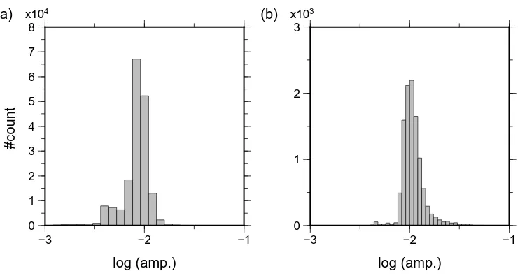
2.4 Amplitude distribution from one night of recordings. (a) Log

ampli-tudes of stack at the center of the grid. (b) Peak log amplitude for

5-second windows. . . 13

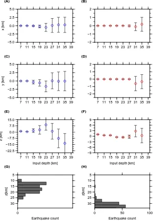
2.5 The location errors derived from synthetic tests. The Left and right

columns are for input sources withMw=0.5 andMw=1.5, respectively. For each input magnitude, we show the difference between input

and output x, y, and z coordinates in panels A-B, C-D, and E-F,

(11)

2.6 The spatial distribution of earthquake density we derived from a catalog spanning 93 nights of the LB array dataset. (A)-(C) A map

view of event density in the 5-12, 12-20, and 20-32 km depth range.

We normalized the densities in each panel by their maximum value.

We represented areas with intense seismicity by orange and red colors,

and areas devoid of seismicity by yellow and white colors. The NIFZ

surface trace, and the local oilfields are denoted by black and green

dashed lines, respectively. LB: Beach oilfield, LBA:

Long-Beach Airport oilfield, WI: Wilmington oilfield. (D) A vertical

cross-section showing event density along line B-B’ in panel A. We

normalized the counts in each 2 km depth bin by their maxima. The Moho depth is indicated by a green curve, and the uncertainty on this

estimate using previously published results. (E) The seismicity depth

distribution in the LB array dataset. . . 17

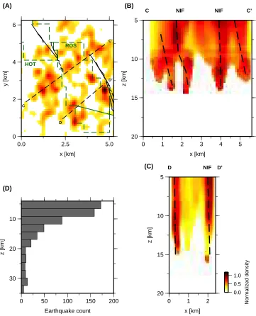
2.7 The spatial distribution of earthquake density from a catalog spanning

25 nights of the Rosecrans dataset. (A) Rosecrans catalog event

density for the depth range 5-35 km. (B)-(C) A vertical cross-section

along lines C-C’ and D-D’ in panel E. We normalized the densities

in panel A by the maximum value, and the density in the

cross-sections by the maximum in 2 km depth bins. (D) The event depth distribution. The location of the NIFZ surface trace, and inferred

faults are indicated by solid and dashed black lines, respectively. The

local oilfields are indicated by green dashed lines. ROS: Rosecrans,

(12)

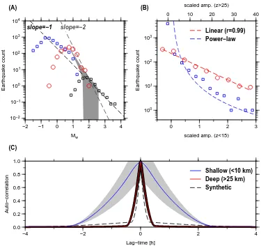
2.8 Temporal analysis and earthquake size distribution in LB. (A) The distribution of earthquake magnitudes. The blue squares and red

circles are for shallow (<15 km) and deep (>25 km) events. Grey

area indicates the expected variability in frequency distributions from

synthetic catalogs with ab-value that lies between 1.7-1.9. The black

squares are for the SCSN catalog, and are normalized according

to the LB array spatio-temporal coverage. The slope of black and

grey curves is equal to -1 and -2, respectively. (B) The distribution

of earthquake signal amplitudes, which we define as the maximum

of the downward-continued, migrated stack in a 5-second window

containing the event, scaled by the maximum of the synthetic stack computed for a collocated source with M_w ₌ 1. We indicated the best fitting exponential model, which appears linear in this

semi-logarithmic scale, by a red curve. The blue curve is a power-law.

(C) The autocorrelation as a function of lag-time between earthquake

rate time-series for shallow (<10 km) at deep (>25 km) clusters. The

blue and red curve indicate the average values we computed for 112

shallow and 52 deep clusters, respectively, with 1-sigma uncertainties

in grey. The black dashed curve is for a synthetic earthquake catalog

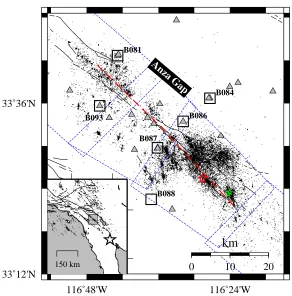
with a random, Poissonian distribution of earthquake occurrences. . . 21 3.1 Location map. Triangles and squares indicate seismic stations and

PBO strain-meters, respectively. Black lines are fault traces and the

red dashed line our assumed fault model. Red, green and white stars

indicate the locations of the M5.4 Collins Valley mainshock, the two

M>4 earthquakes of June 13, 2010, and the M7.2 El Mayor-Cucapah

mainshock, respectively. Blue curves outline the polygons considered

(13)

3.2 Strain data and pre-, co- and post-El Mayor-Cucapah relocated SJF seismicity. Top panel: Cumulative number of events (solid line) and

earthquake rate (vertical bars) as a function of time during 2010. Red,

green, and blue dashed curves indicate the time of the M7.2 El

Mayor-Cucapah, M5.4 Collins Valley, and two M>4 foreshocks, respectively.

Grey regions indicate periods of analysis around both mainshocks

shown in the rows below. Bottom panels: Left and right columns are

for the El Mayor-Cucapah and Collins Valley sequences, respectively.

Second, third, and fourth rows show the differential extensional, areal

and shear strain components, respectively. Horizontal dashed lines

indicate pre- and post-seismically mean strain levels. Vertical bars indicate cumulative post-seismic strains at the end of the analysis

periods (grey bands) and their respective uncertainties. . . 34

3.3 Background seismicity rate and spatial distribution of model cells

for input stress calculation. (a) Background seismicity rate between

January 1, 2001 and April 3, 2010, spatially smoothed with a median

filter of 9 km horizontal width and 1.6 km vertical width. Dashed

polygons indicate areas that contain more than 50 events. (b) Same

as panel a but for the time interval preceding the Collins Valley

mainshock. Blue rectangles indicate cells that contained more than 2 events occurring between April 14 and July 6, 2010. All other

cells have the same background rate as in panel a. (c) Model cells

with available background seismicity rates and >10 (black), 1-10

(grey) and 0 (brown) aftershocks in the 10-day period following the

El Mayor-Cucapah mainshock. (d) Same as panel c for the Collins

Valley aftershocks. . . 40

3.4 Stress errors from synthetic tests. (a) Earthquake rate as a function

of time since the mainshock. Grey curves are for synthetic catalogs

whose inter-event times are drawn from a non-stationary Poissonian distribution with prescribed stress history. Blue and magenta curves

are for the expected rates computed with ˙Nbg= 10

−1_{and ˙}_N

bg= 10

−2

earthquakes/day, respectively, and with ˙N/N˙bg =106, anda =10

−3_.

(b) Stress error computed as the mean difference between stresses

inferred from synthetic catalogs and the actual stresses, normalized

(14)

3.5 Space-time seismicity diagrams for the El Mayor-Cucapah sequence. (a) Aftershock locations projected along fault strike as a function

of time since the mainshock. The symbol color and size indicate

depth and magnitude, respectively. (b) Cumulative event count as a

function of time since the El Mayor-Cucapah earthquake in the NW

(red) and SE (blue) clusters, defined as segments spanning locations

0-30 km and >30 km along-strike in panel a, respectively. Grey

bands indicate intervals of rapid strain rate changes identified in the

strain-meter data (Figure 3.7). . . 45

3.6 Space-time seismicity diagrams for the Collins Valley sequence.

Dashed curve indicates migration velocity that decays as 1/t, where

t is time since the mainshock. See the caption of the previous figure

for details. . . 46

3.7 Temporal evolution of principal strains. Top and bottom rows are for

the El Mayor-Cucapah and Collins Valley sequences, respectively.

(a)-(b) Azimuth of the largest principal strain direction as a function

of time since the mainshock. (c)-(d) Second invariant of the strain

tensor as a function of time since the mainshock. Station names

are indicated in the rightmost column. Vertica grey bands indicate

abrupt strain rate changes at periods corresponding to seismicity rate changes (Figure 3.5b and 3.6b). . . 48

3.8 Top row: The square root of the regularization termC2as a function

of the square root of the joint misfit C1. Bottom row: Square root

ofC1as a function of the constitutive parameter a. The color scale

indicates the value of the smoothing coefficient β. Left (a, c): El

Mayor-Cucapah. Right (b, d): Collins Valley. Green circles indicate

the preferred solutions. . . 53

3.9 Inferred afterslip distributions. (a) El Mayor-Cucapah. (b) Collins

Valley. Triangles indicate along-strike location of PBO strain-meters. Star indicates location of the Collins Valley mainshock. Grey circles

indcate the location of aftershocks projected onto the SJF strand. (c)

Slip contours of afterslip triggered by the El Mayor-Cucapah (red)

(15)

3.10 Observed and modeled strains and surface displacements for the El Mayor-Cucapah (left) and Collins Valley (right) sequences. Dashed

black line indicates the modeled fault trace. Top row: Observed and

modeled strains are indicated by red and blue crosses, respectively.

Location of observed strains are offset for clarity. The dashed

poly-gons indicate the area covered by the bottom panels. Bottom row:

Observed and predicted (using slip models in Figure 3.9) surface

dis-placements at nearby GPS sites are indicated by red and blue vectors,

respectively. 1-σuncertainties are indicated by the red circles. . . 55

3.11 Observed and modeled stresses for the El Mayor-Cucapah (top) and

Collins Valley (bottom) sequences. Left, middle and right columns are for the inversion input, stress residuals (using the models in Figure

3.9), and output on-fault stresses, respectively. Note the color scale

difference between the rightmost and middle columns. . . 56

3.12 Earthquake rates and stresses along the SJF. (a) Seismicity rates as

a function of distance along fault strike, from 7 to 14 days (red) and

from 14 to 94 days (blue) after the El Mayor-Cucapah earthquake. (b)

Cumulative shear stresses inferred from seismicity rates as a function

of distance along fault strike, from 0 to 14 days (red) and from 14 to

94 days (blue) after the El Mayor-Cucapah earthquake. Calculations were done using a = 1× 10−3. Blue and black stars indicate the location of the July 7, 2010, M5.4 Collins Valley, and the June 13,

2010 M>4 earthquakes, respectively. Seismicity rates and stresses

are averaged between 12 and 15 km depth. . . 60

3.13 Amplitude of shear stress differences between cumulative stresses

due to Collins Valley aftershocks and stresses due to the Collins

Valley afterslip. Differences are normalized by the stresses due to

afterslip. Contours are for the afterslip distribution in Figure 3.9. . . . 64

3.14 Temporal evolution of direct and secondary aftershocks. (a) Observed and modeled aftershock counts for the Collins Valley aftershock

se-quence. (b) The fraction of secondary aftershocks as a function of

(16)

3.15 Normalized difference between the afterslip distribution in Figure 3.9 and slip from joint inversion with stresses inferred from direct

after-shock rates (Figure 3.14). Differences are normalized by the best fit

slip distribution. (a) Spatial distribution. Contours indicate inverted

afterslip distribution. Star indicates the Collins Valley mainshock

hypocenter. (b) Histogram of normalized residuals. . . 67

3.16 Norm of the solution scaled by the value of β as a function of the

residual norm for inversions assuming on-fault aftershocks. Solid

black and blue curves are forΩ/Kk k =10 andΩ/Kk k =100,

(17)

C h a p t e r 1

INTRODUCTION

Elucidating the physical processes governing slip at the bottom edge of seismogenic

faults is important for understanding the underlying mechanisms of earthquake

nucleation, propagation, and arrest. However, due to the limited sensitivity of

surface monitoring systems, the spatiotemporal evolution of slip at the

brittle-ductile transition zone, and the coupling between seismic and aseismic slip at

large depths, are not well resolved. This dissertation describes research focused on utilizing seismological and geodetic observations to better constrain a range of

processes occurring at the roots of continental seismic faults. In order to improve

our understanding of the physical processes governing deep fault slip, we have

developed methodologies to process large, dense seismic array data, and to improve

the resolution of geodetic inversions by incorporating information on the space-time

evolution of seismicity.

Dense array seismology is an emerging field in earthquake source studies. Because

the array sensor spacing is two orders of magnitude smaller than conventional seis-mic networks, it allows us to resolve the incoming wave-field at frequencies as high

as 10 Hz. This attribute, together with the large number of sensors (>1000), makes

such arrays ideal for purposes of microseismic monitoring, which is the primary

tool for illuminating active faults. The quality of the seismic catalog is measured by

its magnitude of completeness,Mc, defined as the magnitude above which all

earth-quakes are registered by the network. Earthearth-quakes obey a scaling law according to

which for each unit drop in magnitude the number of events increases by roughly

ten-fold, therefore reducingMcin a given area by one unit will reduce the time needed

for effective seismic monitoring by a factor of ten. Due to seismic attenuation, waves emitted from events occurring near the bottom edge of the seismogenic zone,

the area in which large ruptures are thought to initiate, are more difficult to detect

than ones emitted from shallower depths. In addition, recent observations of deep

seismicity on crustal faults suggest that their size distribution falls off more rapidly

than a power law. If deep crustal earthquakes obey a characteristic distribution, then

their detection will become even more challenging, as the population is dominated

by very small, albeit frequent, microearthquakes. The dense array methodology

(18)

op-portunity to resolve dynamic processes at depths and scales that are inaccessible to a sparse local network.

In Chapter 1, we describe a new methodology for efficient, simultaneous analysis

of thousands of seismic channels. We apply this methodology to dense array data

recorded near the Newport-Inglewood Fault Zone (NIFZ). This technique enabled

us to reduce Mc in the target area by 2 units. The new catalog illuminates a

transition from a diffused zone of deformation in the upper crust to a narrow (∼ 1

km) seismically active zone that extends into the lithospheric mantle beneath the

mapped trace of the NIFZ. Our observations uniquely constrain the spatial extent and degree of shear localization within the seismogenic crust and upper mantle, which

are parameters that are usually very poorly determined. In addition, the catalog

offers an opportunity to study the transition in earthquake scaling properties across

the brittle-ductile transition zone. Our analysis demonstrates that the transition to

a ductile deformation regime has profound implications on earthquake relaxation

mechanisms, and style and degree of earthquake interaction along the NIFZ.

Geodetic inversions, which are the most important tool for mapping fault slip at

depth, are routinely performed in a variety of tectonic environments, and used to constrain pre-, co-, and post-seismic deformation. Because of the large number

of unknowns, slip inversions are underdetermined, and their solutions are

non-unique. This issue is usually addressed by imposing smoothness constraints, which

stabilizes the inversion at the expense of reducing its resolution. As a result,

slip on deep fault segments (below 5 km in the case of near-vertical strike-slip

faults) is usually very poorly resolved. To understand the mode of slip along

deep fault portions, information on the location and timing of microseismicity is

often used in conjunction with fault slip maps. Due to elastic interactions, the

space-time patterns of seismicity are strongly tied to fault slip, and hence changes in earthquake occurrence are expected to reflect variations in underlying processes that

control rupture nucleation, propagation, and arrest. Not only is the incorporation of

seismicity helpful in resolving the fine scale characteristics of slip, it also allows us to

quantify the style and degree of stress transfer from aseismic regions to seismically

active areas, which, in turn, helps constrain the physics that govern deep fault slip.

In Chapter 2 we present an approach that accounts for time-dependent changes in

fault slip and stress via a joint inversion of strain and seismicity data. Seismicity rate response to a stress change is quantified through a constitutive relation which

(19)

the fault’s constitutive parameters, and thus to gain important insights onto physical mechanisms controlling slip. We have applied this approach to study transient slip

events along the Anza segment of the San-Jacinto Fault. The results provide detailed

slip maps at depths that are inaccessible to the surface geodetic network, and allow

us to constrain the mode of static stress-transfer to seismically active fault segments.

Our study shows that earthquake interactions are less important than aseismic slip

for understanding the evolution of seismicity during the sequence. Additionally,

the new on-fault stress maps are used to address the scale and amplitude of loading

along the Anza Gap, a 35-km long segment which is expected to fail in a Mw > 7

(20)

C h a p t e r 2

IMAGING MICROSEISMICITY WITH DENSE SEISMIC

ARRAYS

2.1 Introduction

Earthquakes occurring along transform plate boundaries are generally confined to

the upper portions of the crust, with upper-mantle deformation being predominantly

aseismic (Maggi et al., 2000). Seismological investigations of active faulting at

lower-crustal depths are limited by highly attenuated signals whose level barely

exceeds the noise at the Earth’s surface, and by the sparseness of regional seismic

networks. Consequently, important physical parameters characterizing the transition

from brittle fracture to ductile flow at the base of the seismogenic zone are generally

very poorly determined (Bürgmann and Dresen, 2008).

Because seismic tomography usually cannot resolve features whose spatial extent is less than about 10 km in the mid-lower crust (Thurber et al., 2006; Kahraman

et al., 2015; Shaw et al., 2015), the occurrence of localized shear at those depths is

largely inferred from geological observation of ancient shear zones, where tectonic

deformation can be accommodated within a region whose thickness does not exceed

2 km (Norris and Cooper, 2003). The presence of fault-generated melt in the form

of pseudotachylytes injected into exposed mylonites, and the inferred subsequent

ductile deformation of the two, indicate that seismic slip may occur within largely

aseismic deep shear zones (White, 2012). This is often interpreted as resulting from

ruptures that nucleate at shallow depth but penetrate into the deep ductile region enabled, for example, by thermal weakening mechanisms (Rice, 2006). Here, in

contrast, we present evidence of significant seismicity that nucleates at lower-crustal

to upper-mantle conditions along the Newport-Inglewood Fault Zone (NIFZ). Next,

we describe the seismotectonic setting of the NIFZ.

2.2 Seismotectonic Background

The Los Angeles (LA) basin is a deep sedimentary basin traversed by several active

faults, among which the NIFZ, a major boundary fault in southern California. The

NIFZ is well manifested by a series of small hills trending to the NW that extend

for about 64 km between Culver City and Newport Beach (Figure 2.1). Since it

(21)

extensively, and this has revealed a complex fault geometry that consists of several overlapping en-echelon strike-slip faults which cut through the oil bearing anticlines

(Barrows, 1974; Bryant, 1988; Wright, 1991). In Long Beach (LB), tectonic motion

is primarily accommodated by a single strand known as the Cherry Hill Fault, which

is a right-lateral strike-slip fault. It is sub-vertical down to about 5 km, but may dip

as much as 60◦at larger depths (Wright, 1991).

While reflection seismic surveys provide extensive data on the geometry of the

NIFZ above 5 km, the structure of the NIFZ at larger depths is not well resolved,

thus obtaining precise earthquake locations at those depths is important for hazard mitigation. The spatiotemporal distribution of microseismicity provides valuable

information on the mechanics of fault slip and earthquake interactions, and

nucle-ation (Rubin, Gillard, and Got, 1999; Rubin, 2002; Ziv, 2006; Bouchon, Karabulut,

et al., 2011; Bouchon, Durand, et al., 2013). Activity is LB is not easily associated

with the NIFZ, and occurs primarily to the NE of the fault (Figure 2.1), with the

largest recorded event being the 1933 Mw6.4 LB earthquake, located about 10 km SE of LB (Hauksson and Gross, 1991).

The NIFZ, which hosts many deep earthquakes, is unusual in that it does not display the strong compression, relatively low heat-flow, or strong topographical relief

asso-ciated with deep faults in southern California (Bryant and Jones, 1992; Magistrale,

2002; Hauksson, 2011). Moreover, given the local geotherm (∼ 32◦C/km (Price, Pawlewicz, and Daws, 1999)), deep NIFZ seismicity nucleates at depths where

typical continental crustal rocks are expected to deform in a ductile manner. To

un-derstand the long-term mode of seismic deformation along that fault, we examined a

relocated earthquake catalog from the Southern California Seismic Network (SCSN)

(Hauksson, Wenzheng, and Shearer, 2012). We observed a systematic variation in

the spatial pattern of microseismicity along the NIFZ strike, which we attribute to a transition in faulting style. Earthquake epicenters are tightly clustered on en-echelon

strike-slip faults northwest of LB, but do not follow the mapped trace of the NIFZ to

the southeast of LB (Figure 2.1A). From NW to SE, earthquake density decreases

and maximum earthquake depth, which we define as the depth above which 95%

of seismicity occurs, increases from 10 to 17 km. Along the same section, Moho

depth decreases by about 5 km (Figure 2.1C). The opposite trends of focal and

Moho depths represent an unusual case in which the increase in seismogenic depth

is anti-correlated with crustal thickness (Hauksson, 2011). Finding such deep events

(22)

A

A’

118˚30'W 118˚12'W 117˚54'W

33˚42'N 34˚00'N

0 100 200 Rate 20 km 0 10 20 30 z [km]

0 20 40 60

A ROSE LB A’

Crust Mantle 0 2 4 6 Rc /R a

0 20 40 60

Distance along A−A’ [km]

0 2 4 6 Rc /R a

−20 −10 0 10 20

Distance normal to A−A’ [km]

0

10

20

z [km]

0.0 0.5 1.0

Normalized event count

[image:22.612.157.461.80.497.2]

CA NIF d50 d95 (B) (A) (C) (D) (E)

(23)

Ductile flow laws predict that the depth of the brittle-ductile transition increases with strain rate (Kohlstedt, Evans, and Mackwell, 1995; Hirth and Beeler, 2015). This

should result in a shallower transition along the NIFZ compared to the faster San

Andreas Fault (∼ 2 cm/yr (Lindsey and Fialko, 2013)), assuming similar pressure

and friction coefficient on these two faults. Moreover, if we make the common

assumption that seismicity rate correlates with strain rate, then the observed 50-fold

reduction in earthquake rate recorded by the SCSN from NW of Rosecrans to LB

(Figure 2.1A), should have been accompanied by resolvably shallower seismicity.

In order to improve our understanding of the spatial distribution of anomalous NIFZ

seismicity, we examined earthquake properties in two NIFZ segments that host the

deepest events reported in the regional catalog.

Our study is based on earthquake detection from continuous, simultaneous analysis

of thousands of seismic channels from two dense arrays (Figures 2.1A). We used the

5200-sensor, 7×10 km LB, and 2600-sensor, 5×5 km Rosecrans arrays to compile

catalogs with six and one month of data, respectively. The arrays contain 100 m

spaced, 10 Hz vertical geophones sampling at 500 Hz. Data were down-sampled to

250 Hz, and band-pass filtered at 5-10 Hz. Signals at frequencies above this range

may be affected by spatial aliasing, while analyzing frequencies lower than 5 Hz significantly decreases our spatial resolution. The recordings are contaminated by

various anthropogenic noise sources, such as traffic from local freeways, landing at

the LB airport, trains, and pumping in the LB Oilfield. The volume of the data set

and the characteristics of anthropogenic signals in LB require that event detection be

done automatically. Standard STA/LTA based detection algorithms are inadequate

for our purposes, because such methods depend on the SNR of individual traces,

and are thus easily distracted by spurious signals that originate from shallow noise

sources in the vicinity of the geophones. Given the poor SNR, we turn to seismic

array analysis to detect, locate, and determine the size of seismic events beneath LB. We only analyze nighttime data (6pm-6am), because during these intervals noise

levels in LB significantly decrease.

2.3 Noise Mitigation via Downward Continuation

Our approach for event detection consists of two steps. In the first step we improve the

SNR of the raw data by downward continuation, and in the second we continuously

back-project the downward-continued data to search for coherent high-frequency

(24)

Downward continuation by phase-shift migration (Claerbout, 1976; Gazdag, 1978) is a common imaging technique used in geophysical exploration. We only analyze

vertical component geophones, and thus neglect S-wave energy and use an

approx-imate solution to the scalar (acoustic) wave equation. The acoustic wave field on a

surface,p(x,y,z0,t), is used as a boundary condition to determinep(x,y,z0+∆z,t),

the wave field at depth z= z0+∆z. Assuming a depth-dependent, layered velocity

model, the Fourier transformed data,p(kx,ky,z0, ω), are downward continued to the target depth,zn, with:

p(kx,ky,zn, ω)= p(kx,ky,z0, ω)exp*.

,

−i

n X

j=1

kzjhj+/

-, (2.1)

wherekx andky are the horizontal wavenumbers,ω is the frequency, and hj is the thickness of thej’th depth increment whose velocity isvj. The vertical wavenumber,

kzj, is equal to:

kzj = s

ω2

v2_j

−(k2_x+k2y). (2.2)

Imaginary values of kzj correspond to horizontally traveling evanescent waves.

Their contributions to Equation 2.1 are discarded in our analysis. The space-time

domain representation of the downward continued wave field is obtained by inverse Fourier transformation. In practice, data are downward-continued to a depth of 5

km, for which the velocity model is well constrained from borehole data, and which

is deep enough to suppress surface noise.

Downward continuation assumes the data are uniformly spaced and periodic. To

avoid having wrapped-around signals contaminating the records, the traces and

spatial domain are first zero-padded out to twice and 8-times the spatial and temporal

dimensions of the data, respectively. Furthermore, in order to suppress the influence

of strong spatial variations of SNR on the procedure, the data are first normalized

by its hourly RM S. We interpolate the data to a uniform grid whose cell size is 100× 100 m, by assigning each data point a value equal to an exponentially

weighted sum of its 4 nearest neighbors. Interpolation de-amplifies phases with

high incidence angles that are mostly generated by shallow sources. The amplitude

difference between the raw and interpolated data can be as high as 10% inside the

LB Oil Field, the noisiest area covered by the array, and is at a level of 3-5% in

most other parts of the array. From synthetic tests presented in the Section 2.6,

this procedure has a negligible effect on the location of events in the depth range

(25)

decreases the amplitude of uncorrelated noise relative to coherent signals with high apparent velocities, which are focused back to their origin point at depth. Given the

slow seismic velocities beneath the array and the short inter-station distances, wave

fields with a characteristic frequency of up to about 15 Hz are well resolved by the

LB array.

2.4 Event location via Back-Projection

In the second step of the analysis we back-project the envelope of the

downward-continued data to a volume beneath the array. By stacking the signal’s envelope

we effectively reduce the sensitivity to unknown structure and focal mechanisms.

The envelope, s(t), is defined here by squaring the filtered, normalized, migrated

waveforms, smoothing the squared waveforms using a 18-point (0.072 seconds)

median window, and decimating to a new sampling rate of 50 Hz.

The stacked envelope is defined as:

Si(t)= 1

n

n X

j=1

s(t+τi j), (2.3)

wheren is the number of grid points on the downward-continuation target surface

(same as the number of geophones) and τi j is the P-wave travel time difference

be-tween thej’th downward-continuation grid point and a reference grid point assuming

a source located at thei’th back-projection grid point. When the source-receiver

distance is much larger than the aperture of the array, the wave-front arriving at

the array is typically approximated as a plane-wave. However, given the LB array

geometry and the distance to the sources we wish to image, this approximation is

not valid. We therefore migrate the seismic envelopes and project the energy back

to the origin. Theoretical travel-times are computed on a mesh whose elements are 0.125 km3using a local 1-D velocity model extracted from the SCEC Community Velocity Model - Harvard (CVM-H) (Süss and Shaw, 2003; Plesch et al., 2011).

We analyze the amplitude of the migrated stack to identify coherent energy in the

frequency band of interest. Figure 2.2 presents the raw and downward-continued

waveforms, and spatial distribution of the log of the stack amplitude of anMw =0.4 event whose focal depth is 14 km. Note that the arrivals are only visible after the

data are downward-continued. Figure 2.3 presents the down-continued waveforms

and surface ground motions due to aMw = 0.4 that occurred beneath the Rosecrans array.

(26)

field, which may differ significantly from theoretical travel times computed using a 1-D model. Thus, a detailed 3-D velocity model should improve the accuracy of

hypocentral locations. However, for the expected range of source-receiver distances

in LB, the available 3-D model would only slightly modify the computed travel

times, and hence introduce slight shifts to the locations obtained with a 1-D model.

To confirm that, we compared travel time predictions from the CVM-H velocity

model to the predicted travel times using the 1-D model, and found that the residuals

are up to 5% of the travel time along the path, which would introduce location shifts

that are smaller than our location uncertainties. This suggests that our interpretations

are not strongly dependent on the velocity model we use.

2.5 Probabilistic Approach for Event Detection in Back-Projection Images

The detection procedure is carried out by analyzing the filtered, normalized, downward-continued, stacked envelopes. We stack (delay and sum) the envelopes of the

down-ward continued waveforms for each potential position, window the stack for each

position in our grid with 5-second, non-overlapping windows, construct a

back-projection image from the peak amplitude of each window, and select the location

that corresponds to the maximum of the image. We end up with a time-series

con-taining the maxima of the back-projection image, on which the detection is made.

Figure 2.4a shows the distribution of the logarithm of amplitudes of the migrated

envelopes for a node located in the middle of our grid during one night of recordings.

Figure 2.4b shows the distribution of the maxima in the 5-seconds windows for the same time period. Because the noise is log-normally distributed, the ensemble of

observations containing its maxima belongs to a Gumbel distribution.

A 5-second window is identified as containing a true event if its maximum amplitude

exceeds a threshold corresponding to 5 times the MAD of the distribution of noise.

This value allows us to determine the probability of false detections, which is the

probability that a sample randomly drown from the ensemble of the stack maxima

is actually noise. The probabilities can be computed based on the fact that the stack maxima belongs to a Gumbel distribution, but the signal we wish to detect is

belongs to a power-law or exponential distributions. To estimate the probabilities

we generate 1000 realizations of Gaussian noise whose variance is equal to the

variance in the back-projection images, select the maxima of each realization, and

use a maximum-likelihood estimator to fit the data to a Gumbel distribution. For a

given threshold valueT, the probability of false detection is estimated by using:

(27)

0 5 10 15 20 25 time [s] 1.5 2.0 2.5 3.0 3.5 4.0 4.5 5.0 5.5 6.0 distance [km]

0 5 10 15 20 25

time [s] 0 500 1000 1500 2000 2500 #count 11 12 13 14 15 z [km]

0 1 2 3 4

x [km]

−1.05 −1.00 −0.95 −0.90 log(amplitude) 0 1 2 3 y [km]

0 1 2 3 4

x [km] 0.0 0.5 1.0 1.5 2.0 #count

−3 −2 −1 0

[image:27.612.132.490.128.498.2]

log(amplitude) x102 (e) (d) (c) (a) (b)

(28)

1 3 5

y [km]

1 3 5

x [km]

1.50 sec.

1 3 5

x [km]

2.34 sec.

1 3 5

y [km]

2.46 sec. 2.62 sec.

z=0 km

z=5 km

0 1 2 3 4 5

Time [s]

(E) (C)

(A) (B) (F)

(D)

0.0 0.2 0.4 0.6 0.8 1.0

Time [s] 0.0

0.2 0.4 0.6 0.8 1.0

[image:28.612.141.506.178.474.2]

Distance [km]

(29)

0 1 2 3 4 5 6 7 8

#count

−3 −2 −1

log (amp.)

0 1 2 3

−3 −2 −1

log (amp.) (b) x103

[image:29.612.135.505.102.301.2]

(a) x104

Figure 2.4: Amplitude distribution from one night of recordings. (a) Log amplitudes of stack at the center of the grid. (b) Peak log amplitude for 5-second windows.

where µ and β are the fitting coefficients. The rate of false alarms is obtained

by multiplying the probability by the number of instances on which detection is

preformed. The probabilities that a variable drawn from a Gumbel distribution will

exceed the 5-MAD and 2-MAD thresholds are 3.22×10−7and 1.27×10−4, which translates to a constant rate of about 2×10−3and 1 false alarm per night.

2.6 Location Error Estimation

To estimate the location uncertainty we first compute the surface seismograms due

to a strike-slip point source. We use a 1-D velocity profile extracted from the

SCEC CVM-H model. The synthetic traces are processed in the same fashion as

the real data. We spatially interpolate the seismograms, downward-continue, and back-project the migrated envelopes onto the volume beneath the array. We then

add noise whose distribution is derived from the real data and perform the detection.

Our detection scheme operates on the images maximum amplitudes.

We estimate the location uncertainty from Monte-Carlo simulations. In each

sim-ulation we perturb the amplitudes of the synthetic back-projection images with

log-normally distributed, spatially uncorrelated noise, and extract the location of

(30)

14 −5.0 −2.5 0.0 2.5 5.0 x [km]

7 11 15 19 23 27 31 35 39

−2 −1 0 1 2

7 11 15 19 23 27 31 35 39

−5.0 −2.5 0.0 2.5 5.0 y [km]

7 11 15 19 23 27 31 35 39

−2 −1 0 1 2

7 11 15 19 23 27 31 35 39

(C) (D) −22.5 −15.0 −7.5 0.0 7.5 15.0 z [km]

7 11 15 19 23 27 31 35 39 Input depth [km]

−9 −6 −3 0 3 6 9

7 11 15 19 23 27 31 35 39 Input depth [km]

(E) (F) 5 10 15 20 25 30 z[km] 0 Earthquake count 5 10 15 20 25 30 z[km]

0 50 100

Earthquake count

[image:30.612.148.460.40.489.2]

(G) (H)

Figure 2.5: The location errors derived from synthetic tests. The Left and right columns are for input sources with Mw=0.5 and Mw=1.5, respectively. For each input magnitude, we show the difference between input and output x, y, and z coordinates in panels A-B, C-D, and E-F, respectively. The error bars indicate 1-sigma uncertainties. Focal depth distribution in LB for events with 0.4< Mw < 0.5, andMw > 1.5 are shown in panels G and H, respectively.

report the mean and standard deviation of the output locations. Figure 2.5 presents

the error analysis for synthetic sources whose depth varies between 7 to 35 km.

For events with Mw > 1.5, our procedure accurately recovers the input locations down to depth of about 27 km. The uncertainty on the location of a source located

(31)

vertical and horizontal directions, respectively. The location uncertainty on events withM < 0.5 at depths below 20 km is generally larger, however the majority of the

smallest magnitude events in our catalog occupy shallower depths (Figure 2.5G ).

2.7 Magnitude Determination

In order to determine the magnitude of the detected events we use a simulation-based

calibration scheme. Unfortunately, the regional catalog does not contain any events

that occurred during the survey within the target volume, which forces us to use a

model to calibrate the amplitudes. We compute the surface seismograms due to a

strike-slip point source with Mw = 1 and a 3 MPa stress drop using the frequency-wavenumber wave propagation method of Zhu and Rivera (2002) together with the

velocity and attenuation structure from the CVM-H model. The entire catalog is

calibrated with a single event since the corner frequencies of the reference and recorded events are much higher than the frequencies we analyze. In the same

fashion as the real data, the synthetics are normalized, downward-continued,

back-projected onto the input hypocentral locations, which populate the target volume at 1

and 2 km spacing in the horizontal and vertical directions, and interpolated to a finer

grid using bi-cubic interpolation. Since the raw data are normalized by their hourly

RM S, the process is repeated for the synthetic data using the RM S values of the

raw traces. Our procedure determines event magnitudes from the amplitude ratio

between the observed and synthetic data. Because the synthetic data are produced

with a realistic attenuation model, the procedure does not require that we apply any attenuation corrections.

2.8 Results: Deep Faulting in Long-Beach and Rosecrans

Our catalog illuminates a transition from diffuse seismic deformation in the upper

crust to localized deformation in the lithospheric mantle. Shallow seismicity (<15

km) in LB is diffuse and uncorrelated with the mapped fault trace or with the nearby

oilfield (Figure 2.6A). To the southwest of the main NIFZ strand, we identify a

NW-NNW striking segment that is mostly active between 12 and 20 km, but contains

sparse seismicity outside this depth range. A second structure is located to the

northeast. Below 20 km, this zone is very seismically active, but the location near

the edge of the array prevents us from resolving its geometry in detail.

With increasing depth, seismicity progressively concentrates beneath the mapped

trace of the NIFZ and the width of the seismically active zone decreases (Figure

(32)

directly beneath the mapped trace of the NIFZ. The vertical cross-section (Figure 2.6D) clearly shows that the fault dip below 15 km is near-vertical, and that it retains

this geometry in the upper mantle. In particular, our observations do not support

a previous suggestion that the NIFZ is truncated at shallow depths by an active

detachment fault (Crouch and Suppe, 1993). Accounting for location uncertainties

in our catalog, the deformation zone illuminated by deep LB seismicity is no more

than 2 km wide, consistent with several exhumed mylonite shear zones (Norris and

Cooper, 2003). We also find that deep seismicity (>20 km) accounts for at most

10%-20% of the cumulative long-term moment rate accommodated by the fault,

assuming a slip rate 0.5 mm/year (Grant et al., 1997). Based on these results, we

conclude that aseismic, viscous flow accommodates most of the deformation in the lower crust.

The spatial distribution of deep seismicity varies along the NIFZ strike. Seismicity

in Rosecrans occurs along 4 or 5 strands that form a 5 km wide fault zone, which is

active down to about 15 km, but contains few events below that depth. Unlike the

LB segment, these strands appear to dip at up to 70◦to the northeast (Figure 2.7). Multiple en-echelon strike-slip faults are generally observed at shallower depths

along that section (Wright, 1991), and our study confirms that these structures are active at larger depths. If the Rosecrans catalog is representative of the long-term

deformation along that segment, then the scarcity of deep seismicity suggests that

the zone of deep, localized seismic deformation extends no more than 15 km along

the NIFZ strike to the northwest of LB.

Independent evidence compatible with deep faulting comes from recent

measure-ments of3He/4He, a primary indicator of mantle-derived phases within the crust (Kennedy et al., 1997), in deep boreholes in the LA basin (Boles et al., 2015) (Figure

2.1A and 2.1D-E).3He enrichment is more than twice as high than along the much more tectonically active San Andreas Fault. The observed along-strike trend in the

fraction of mantle derived Helium is remarkably well correlated with the seismicity

depths in the regional catalog. They both first increase towards the southeast, then

decrease somewhat and flatten southeast of LB (Figure 2.1C and 2.1D). Further

evidence of the deep root of the NIFZ comes from the seismic imaging of a sharp

vertical offset in the lithosphere-asthenosphere boundary (Lekic, French, and

Fis-cher, 2011), which extends to a depth of about 90 km beneath the zone of deep

(33)

LB LBA WI NIF B B’ 0 2 4 6 8 10 y [km]

0.0 2.5 5.0 7.5

x [km]

5< z[km]< 12

0.0 2.5 5.0 7.5

x [km]

12< z[km]< 20

0 2 4 6 8 10 y [km]

0.0 2.5 5.0 7.5

x [km]

20< z[km]< 32

0.0 0.5 1.0 Normalized density 5 10 15 20 25 30 z [km]

0 1 2 3 4 5 6 7 8

x [km] NIF B B’ Crust Mantle 5 10 15 20 25 30 z[km] 250 750 1250 Earthquake count (E) (D)

[image:33.612.132.507.75.357.2]

(A) (B) (C)

Figure 2.6: The spatial distribution of earthquake density we derived from a catalog spanning 93 nights of the LB array dataset. (A)-(C) A map view of event density in the 5-12, 12-20, and 20-32 km depth range. We normalized the densities in each panel by their maximum value. We represented areas with intense seismicity by orange and red colors, and areas devoid of seismicity by yellow and white colors. The NIFZ surface trace, and the local oilfields are denoted by black and green dashed lines, respectively. LB: Long-Beach oilfield, LBA: Long-Beach Airport oilfield, WI: Wilmington oilfield. (D) A vertical cross-section showing event density along line B-B’ in panel A. We normalized the counts in each 2 km depth bin by their maxima. The Moho depth is indicated by a green curve, and the uncertainty on this estimate using previously published results. (E) The seismicity depth distribution in the LB array dataset.

between the upper mantle and the crust. These fluids in turn could provide a source

of high pressures that extend the depth of seismic deformation.

2.9 Results: Depth-Dependent Earthquake Size Distribution and Temporal

Clustering

The along-depth variation in the spatial distribution of NIFZ seismicity is most likely

due to a rheological transition, which we expected to manifest itself as a resolvable

(34)

0 2 4 6

y [km]

0.0 2.5 5.0

x [km]

HOT

ROS

C

C’

D

D’

NIF NIF

C C’

5

10

15

20

z [km]

0 1 2 3 4 5

x [km]

10

20

30

z [km]

0 50 100 150 200

Earthquake count

5

10

15

20

z [km]

0 1 2

x [km]

D NIF D’

0.0 0.5 1.0

Normalized density

(C)

(D)

[image:34.612.143.504.88.534.2]

(A) (B)

(35)

temporal clustering of LB seismicity. Because our spatial resolution is limited by location uncertainties that are likely larger than the rupture dimensions of the

earthquakes we imaged, we focused on aspects of the population’s temporal and size

distributions which varied on scales of several hundred meters.

We can investigate the degree of earthquake interaction using the ratio between the

number of small and large earthquakes, commonly characterized by the b-value

(b = −dlog10(N)/dM, where N is the number of earthquakes of magnitude larger

than M). In most tectonic environments b-values vary between 0.8 and 1.5 and

decrease with increasing deviatoric stress (Scholz, 2015). Larger b-values are associated with an increase in ductility, and a reduction of fault strength, both in the

lab (Scholz, 1968) and on natural faults (Spada et al., 2013). Recent observations

of Low-Frequency Earthquakes (LFE), whose collective failure results in tectonic

tremors, suggest that their number fall off rapidly with size (estimated from tremor

amplitudes). Those studies suggest that LFE numbers are better described by

an exponential distribution (Watanabe, Hiramatsu, and Obara, 2007; Shelly and

Hardebeck, 2010; Sweet, Creager, and Houston, 2014), or a very steep power-law

(Bostock et al., 2015). The rapid fall-off in LFE numbers with increasing size

is similar to deep NIFZ seismicity. However, unlike other areas, the NIFZ catalog captures a depth-dependent transition in earthquake properties (Figure 2.8A-B). The

distribution of shallow (<15 km) earthquakes in the 6 months period is consistent

with that of the 30-years spanning SCSN catalog.

Note that for b > 1.5, the integral over the frequency-magnitude distribution does

not converge at the limit of very small magnitudes (e.g. Molnar, 1979). However,

as shown in Figure 2.8B, the deep event population is better fitted by an exponential

distribution. This ensures that the integral over the event counts does converge even

at a magnitude range which is below our detection level.

Spatio-temporal clustering is ubiquitous in earthquake catalogs and manifests most

strikingly in the form of mainshock-aftershock sequences. We can model seismic

activity as a random Poissonian process because it decorrelates at large distances or

long time intervals. To determine if this behavior is depth-dependent, we analyzed

the temporal autocorrelation functions of the spatially smoothed earthquake rates

at different depth ranges. To estimate the degree of temporal clustering we divide

the volume into shallow (<10 km) and deep (>25 km) depth ranges, and bin the events at 2.5×3 km, and 3×4.5 km cells, respectively. For each depth range and for

(36)

the rate functions at 2-minute bins using linear interpolation, zero-pad the rates on both ends, compute their autocorrelation function, and stack the autocorrelations for

each depth range. The autocorrelation function of a random process should appear

as a zero-peaked delta function. The increase in degree of temporal clustering for

shallow event clusters causes the stacked autocorrelation function to decay more

gradually relative to the one computed for the deeper clusters.

We use larger bins for deeper events to ensure that the number of events in these

clusters is not significantly different than the size of shallow clusters. However, the

total number of deep events is only about 30% of the number of shallow events, which may bias our results. In addition, some artifacts are introduced into the

autocorrelation analysis due to zero-padding of short sequences. We address these

issues by analyzing a synthetic catalog in which event times are drawn from a

Poissonian distribution, and whose temporal distribution is similar to the distribution

of the deep events clusters (i.e. about 6-7 events per cluster, with average inter-event

times of about 1.5 hours). We compute the rates of each simulated sequence, and, in

the same fashion as the real data, compute and stack the autocorrelation functions.

The dashed black curve in Figure 2.8C presents the results of the analysis using

30 simulated clusters. We find that the temporal distribution of deep earthquake clusters resembles more a random, Poissonian process than the distribution of the

shallow event clusters.

To conclude, deep earthquake occurrence shows weak temporal correlation and

resembles a random Poissonian process. This indicates diminished earthquake

interactions at these depths.

2.10 Interpretation

Models of lithospheric strength may explain deep NIFZ seismicity while

incorporat-ing constrains on lower crustal rheology (Hirth and Beeler, 2015). However, relevant

parameters such as temperature, grain size, lithology, and water content are generally poorly constrained. One possibility is that lateral as well as vertical compositional

changes in the lower crust will promote brittleness within ductile, generally aseismic

regions. A line of evidence supports the existence of considerable heterogeneity in

material properties at lower-crustal to upper-mantle depth beneath the NIFZ. These

include the observation of a sharp offset in the lithosphere-asthenosphere boundary

extending to 90 km depth beneath the NIFZ (Lekic, French, and Fischer, 2011), a

(37)

0.0 0.2 0.4 0.6 0.8 1.0

Auto−correlation

−4 −2 0 2 4

Lag−time [h] 10−2

10−1

100

101

102

103

104

Earthquake count

slope=−1 slope=−2

−2 −1 0 1 2 3 4

Mw

100

101

102

103

Earthquake count

0 1 2 3

scaled amp. (z<15)

Linear (r=0.99) Power−law

Shallow (<10 km) Deep (>25 km) Synthetic

0 10 20 30 40

scaled amp. (z>25)

(B) (A)

[image:37.612.131.506.103.459.2]

(C)

(38)

2013), travel-time tomography showing a fast, possibly mafic body starting at∼18 km beneath the LA basin (Hauksson, 2000), magnetic profiles suggesting that the

NIFZ is the southern boundary of an ultramafic body (Romanyuk, Mooney, and

De-tweiler, 2007), and along-strike variations in the orientation of the principal stress

axes (Hauksson, 1987), the distribution of mantle Helium (Boles et al., 2015), and

near-surface (Wright, 1991) and deep faulting styles. Structural factors may also

assist slip localization. The fabric of foliated mica schists, which are thought to be

distributed at lower crustal depths beneath California (Porter, Zandt, and McQuarrie,

2011; Audet, 2015), possibly contain discrete surfaces accommodating seismic slip.

Unstable frictional sliding of mafic rock has been observed in lab experiments (King

and Marone, 2012; Mitchell, Fialko, and Brown, 2015), and in the field. (Ueda et al., 2008; Matysiak and Trepmann, 2012). This behavior may be further encouraged in

the presence of fluids, either by reducing the effective normal stress or by promoting

strain localization in narrow shear bands (Getsinger et al., 2013), perhaps akin to

the localized deformation zone we imaged beneath LB (Figure 2.6C).

The rheological transition has profound implications on the degree of fault

local-ization, relaxation mechanisms, and earthquake scaling properties. We can

recon-cile these observations with a conceptual framework in which deep deformation is predominately accommodated by ductile flow but interspersed by seismogenic

asperities. Seismic rupture nucleated in a brittle asperity can penetrate into the

surrounding region, up to a certain distance that generally depends on the

asper-ity size and stress drop and on the resistance of the matrix. This effective radius

Re controls the range of interaction between asperities. The ratio between Re and

inter-asperity distance ∆ determines the ability of asperities to break together in

seismic events, despite the intervening creep, and thus the statistics of the

earth-quake catalog. When Re/∆is large, ruptures can involve multiple asperities. This

strong interaction regime potentially leads to a scale-free, power-law earthquake size distribution (Figure 2.8A) and temporal clustering (Figure 2.8C), as observed

at shallow depths. When Re/∆is small, asperities tend to break in isolation. In this

weak interaction regime seismicity is temporally uncorrelated and, if asperities have

a characteristic size, the earthquake size distribution is scale-bound, as observed in

the deep NIFZ beneath LB. A systematic decrease of Re/∆with increasing depth

may result from several processes, which are not necessarily independent. One

possibility is a rheological control: Re may decrease with depth due to increasing

velocity-strengthening of the creeping matrix or decreasing stress drop within the

(39)

the range of asperity sizes (and hence of Re) may be narrower or∆may be larger,

due for instance to lithological variations.

References

Audet, Pascal (2015). “Layered crustal anisotropy around the San Andreas Fault near Parkfield, California”. In: J. Geophys. Res. 120.5, pp. 3527–3543. issn_:

2169-9313.doi_:_{10.1002/2014JB011821}_.

Barrows, A G (1974). “A review of the geology and earthquake history of the Newport-Inglewood structural zone, southern California”. In:Calif. Div. Mines Geol. Spec. Rept.114.

Boles, J. R. et al. (2015). “Mantle helium along the Newport-Inglewood fault zone, Los Angeles basin, California: A leaking paleo-subduction zone”. In:Geochem. Geophys. Geosyst.16.7, pp. 2364–2381.doi_:_{10.1002/2015GC005951}_.

Bostock, M. G. et al. (2015). “Magnitudes and moment-duration scaling of low-frequency earthquakes beneath southern Vancouver Island”. In:J. Geophys. Res. 2015JB012195.doi_:_{10.1002/2015JB012195}_.

Bouchon, M., V. Durand, et al. (2013). “The long precursory phase of most large in-terplate earthquakes”. In:Nature Geo.6.4, 299–302.doi_:_{{10.1038/NGEO1770}}_.

Bouchon, M., H. Karabulut, et al. (2011). “Extended Nucleation of the 1999 M-w 7.6 Izmit Earthquake”. In:Science331.6019, 877–880. doi_:_{{10.1126/science.}

1197341}.

Bryant, B. (1988). “Recently active traces of the Newport-Inglewood fault zone, Los Angeles and Orange Counties”. In:Calif. Div. Mines Geol. Open-File Rept. 88-14.

Bryant, B. and L. Jones (1992). “Anomalously deep crustal earthquakes in the Ventura Basin, southern California”. In: J. Geophys. Res.97.B1, pp. 437–447.

issn_{: 2156-2202.} doi_: _{10.1029/91JB02286}_.url_:_{http://dx.doi.org/10.}

1029/91JB02286.

Bürgmann, R. and G. Dresen (2008). “Rheology of the Lower Crust and Upper Mantle: Evidence from Rock Mechanics, Geodesy, and Field Observations”. In: Annu. Rev. Earth Planet. Sci. 36.1, pp. 531–567. doi_: _{10 . 1146 / annurev .}

earth.36.031207.124326.

Claerbout, J F (1976).Fundamentals of geophysical data processing : with applica-tions to petroleum prospecting. McGraw-Hill.

Crouch, J K and J Suppe (1993). “Late cenozoic tectonic evolution of the Los-Angeles basin and Inner California Borderland - A model for core complex like crustal extension”. In:Geo. Soc. Am. Bull.105.11, 1415–1434.doi_:_{10.1130/

(40)

Gazdag, J. (1978). “Wave-equation migration with phase-shift method”. In: Geo-physics43.7, 1342–1351.doi_:_{{10.1190/1.1440899}}_.

Getsinger, A. J. et al. (2013). “Influence of water on rheology and strain localization in the lower continental crust”. In:Geochem.Geophys.Geosyst. 14.7, pp. 2247– 2264.issn_{: 1525-2027.}doi_:_{10.1002/ggge.20148}_.

Grant, L B et al. (1997). “Paleoseismicity of the north branch of the Newport-Inglewood fault zone in Huntington Beach, California, from cone penetrometer test data”. In:Bull. Seis. Soc. Am.87.2, 277–293.

Hauksson, E. (1987). “Seismotectonics of the Newport-Inglewood fault zone in the Los-Angeles basin, southern California”. In: Bull. Seismol. Soc. Am. 77.2, pp. 539–561.

– (2000). “Crustal structure and seismicity distribution adjacent to the Pacific and North America plate boundary in southern California”. In: J. Geophys. Res. 105.B6, pp. 13875–13903.doi_:_{10.1029/2000JB900016}_.

– (2011). “Crustal geophysics and seismicity in southern California”. In:Geophys. J. Int.186.1, pp. 82–98.doi_:_{10.1111/j.1365-246X.2011.05042.x}_.

Hauksson, E. and S. Gross (1991). “Source parameters of the 1933 Long-Beach earthquake”. In:Bull. Seis. Soc. Am.81.1, 81–98.

Hauksson, E., Y. Wenzheng, and P. M. Shearer (2012). “Waveform Relocated Earth-quake Catalog for Southern California (1981 to June 2011)”. In: Bull. Seismol. Soc. Am.102.5, pp. 2239–2244.doi_:_{10.1785/0120120010}_.

Hirth, Greg and N. M. Beeler (2015). “The role of fluid pressure on frictional behavior at the base of the seismogenic zone”. In:Geology 43.3, pp. 223–226.

issn_{: 0091-7613.}doi_:_{10.1130/G36361.1}_.

Kahraman, M. et al. (2015). “Crustal-scale shear zones and heterogeneous structure beneath the North Anatolian Fault Zone, Turkey, revealed by a high-density seis-mometer array”. In:Earth Planet. Sci. Lett.430, pp. 129–139.issn_{: 0012-821X.}

doi_:_{http://dx.doi.org/10.1016/j.epsl.2015.08.014}_.

Kennedy, B. M. et al. (1997). “Mantle fluids in the San Andreas fault system, California”. In:SCIENCE 278.5341, pp. 1278–1281.issn_{: 0036-8075.}doi_:_10.

1126/science.278.5341.1278.

King, D. S. H. and C. Marone (2012). “Frictional properties of olivine at high temperature with applications to the strength and dynamics of the oceanic litho-sphere”. In:J. Geophys. Res.117.doi_:_{{10.1029/2012JB009511}}_.