Complete Tree Subset Difference Broadcast Encryption Scheme
and its Analysis
Sanjay Bhattacherjee and Palash Sarkar Applied Statistics Unit
Indian Statistical Institute
203, B.T.Road, Kolkata, India - 700108. {sanjayb r,palash}@isical.ac.in
Abstract
The Subset Difference (SD) method proposed by Naor, Naor and Lotspiech is the most popular broadcast encryption (BE) scheme. It is suitable for real-time applications like Pay-TV and has been suggested for use by the AACS standard for digital rights management in Blu-Ray and HD-DVD discs. The SD method assumes the number of users to be a power of two. We propose the Complete Tree Subset Difference (CTSD) method that allows the system to support an arbitrary number of users. In particular, it subsumes the SD method and all results proved for the CTSD method also hold for the SD method. Recurrences are obtained for the CTSD scheme to count the number, N(n, r, h), of possible ways r users in the system ofn users can be revoked to result in a transmission overhead or header length of h. The recurrences lead to a polynomial time dynamic programming algorithm for computing N(n, r, h). Further, they provide bounds on the maximum possible header length. A probabilistic analysis is performed to obtain an O(rlogn) time algorithm to compute the expected header length in the CTSD scheme. Further, for the SD scheme we obtain an explicit limiting upper bound on the expected header length.
Keywords: Broadcast encryption; subset difference; combinatorial analysis; recurrence; probabilistic analysis; expected header length; transmission overhead; asymptotic analysis
1
Introduction
A Broadcast Encryption (BE) scheme allows a centre to efficiently broadcast encrypted information so that only an intended set of users can recover the message. Before the system starts to work, the users are given some secret information. This could be the actual decryption keys or some information from which it can derive the decryption keys. A user uses this information for decrypting relevant encrypted digital content. Copyright protection using Digital Rights Management (DRM) techniques is an important application of BE. The application of BE systems is pretty wide in the implementation of DRM for content protection in digital data distribution technologies such as pay-TV, Internet or mobile video broadcast, optical discs, etc.
In a typical BE scheme, the entire digital data to be broadcast is divided into blocks. Each such block is called a message. Each message to be broadcast, is encrypted using a unique key called a session key. The session key in turn, is encrypted a number of times using user keys and these multiple encryptions of the session key are sent as theheader of the encrypted message. The transmission overhead of the scheme is determined by the number of encryptions of the session key in the header. This is called theheader length and we denote this quantity byh.
In a fully resilient scheme, even if an adversary has the decryption keys of all the remaining non-privileged users in the system, it will not be able to correctly decrypt the content. The non-privileged users are called
1 INTRODUCTION 2
revoked users. A crucial requirement for a BE scheme is that it should facilitate dynamic revocation of decryption privilege from any subset of users at any point of time. The decision could be based on their subscription or privilege status.
In real-time scenarios like Pay-TV, Internet or mobile video broadcast, the number of users can vary from a few thousands to millions. For other real-time applications of BE like broadcasting secret instructions to military outposts from a base station, the number of users will be a few hundreds. The BE scheme that is used in real time scenarios as above, has to be efficient in terms of the transmission overhead associated with each message as also the encryption and decryption times and storage of user keys. For non-real-time applications like content protection in Blu-Ray discs and HD-DVDs, the requirements from a BE scheme are somewhat different. Here, the transmission overhead is the additional information stored in the physical media that is used for decrypting the content. Storage space in discs is no more a constraint nowadays. Further, since encryption does not happen in real-time, improving the encryption time is also not very important. On the other hand, reducing the user storage and decryption time is still important.
Broadcast Encryption was introduced in [Ber91] followed by [FN93]. There have been several works in this area [Sti97, SW98] since then, but the most popular scheme out of these is the tree-based Subset Difference (SD) method of [NNL01]. Since it is a symmetric key based scheme, it is very efficient in terms of encryption and decryption time. It allows the users to be stateless and hence, they do not have to update their individual secret information with every session. It also allows dynamic revocation of users. User storage requirement is
O(log2n) where nis the total number of users and the transmission overhead is linear in the number of revoked usersr. Currently, the SD scheme offers the simplest algorithm and the best trade-offs for use in both real-time applications like Pay-TV and non-real time applications like content protection in optical discs [AAC].
1.1 Our Contributions
There are three contributions in this work.
Arbitrary number of users: We broaden the scope of use of the SD scheme. The SD scheme and all follow-up works [HS02, GST04, PB06, AK08, MMW09] assume the total number of users n to be a power of two. When implementing the SD scheme for applications such as Pay-TV, it is possible that the number of users in the system will be arbitrary. In that case, the centre has to assume the existence of dummy users to make the number of users a power of two. We relax this restriction to allow any arbitrary number of users in the system by introducing the Complete Tree Subset Difference (CTSD) scheme. The CTSD scheme is based on the SD scheme and subsumes it while eliminating the requirement of dummy users in the system. When the number of users in the CTSD method is a power of two, it becomes exactly the same as the SD scheme. Inclusion of dummy users results in the expected header length of the SD scheme to be more than the CTSD scheme for practical values of nand r.
It is to be noted that an implementation that uses the SD scheme can easily shift to using the CTSD scheme with minimal change in the software implementation. This is because the internal tree structure used for assigning keys to subsets of users in the SD scheme remains almost the same in the CTSD scheme.
Combinatorial Analysis: The importance of the SD scheme motivates the study of its combinatorial prop-erties. We carry out such a study for the CTSD scheme and the results so obtained also apply to the SD scheme. A new approach is used for the detailed combinatorial analysis. A method is proposed to count the number,
1 INTRODUCTION 3
method, one would have to run the SD algorithm on the possibly exponentially many nr
revocation patterns. Further combinatorial results that we obtain are as follows.
1. The worst case header length for a givenrin the SD scheme was shown to be 2r−1 in [NNL01]. We show that the worst case header length for the CTSD scheme and hence for the SD scheme is min(2r−1,⌊n/2⌋, n−r).
2. Given r, we characterize the minimum number of users, nr, that need to be in a system using the CTSD
method, that can give rise to the maximum header length of 2r−1. For the special case of the SD method the expression fornr was obtained in [MMW09].
3. For the special case when nis a power of two i.e., for the SD scheme, we use the recurrences to obtain a generating function for the sequence. Earlier, a generating function of a slightly different form was obtained in [PB06] using direct arguments.
Probabilistic analysis: We propose a simple and efficient algorithm for computing the expected header length for a given n and r in the CTSD and hence the SD method. The algorithm requiresO(rlogn) multiplications and O(1) space. Due to its efficiency, this algorithm allows the computation of the expected header length for values of n ranging from a few hundreds to millions. This provides a useful tool to practitioners implementing either the SD or the CTSD method.
For the SD scheme, asngoes to infinity through powers of two, we provide an expressionHrfor the limiting
upper bound on the expected header length Hn,r. The value of Hr can be computed using O(r) multiplications.
Computing this value for different r shows that Hr is always less than 1.25r. The only previously known upper
bound on the expected header length in the SD scheme for r revoked users was proved to be 1.38r in [NNL01]. They also commented that experimental results indicated that the bound is probably 1.25r. Our analysis of the expected header length shows that proving the precise limiting upper bound is more complicated than anticipated in [NNL01].
1.2 Previous Works
The tree-based SD scheme has inspired quite a lot of work in the area of broadcast encryption. Asymptotic improvements to the user storage parameter of the SD scheme were suggested in the tree-based LSD scheme of [HS02] with some loss of efficiency in the transmission overhead. Analysis of the combinatorics behind broadcast encryption schemes and different generic bounds on the efficiency parameters have been done in [LS98, PGM04] and other works. A generic method for constructing BE schemes from pseudo-random generators was proposed in [AKI03].
An analysis of the expected header length of the SD and LSD schemes was done in [PB06]. As mentioned earlier, they proposed generating functions for counting the number of ways pusers out of total n users can be given access privilege so that the header length will be h. Using this generating function, they found equations to compute the expected header length for a given nand r. However, they admitted that their equations were “complex to compute and difficult to gain insight from”. Consequently, they went forward to findapproximations
for the same. The analysis of the expected header length in [PB06] was continued in [EOPR08] to show that the standard deviations are small compared to the means as the number of users gets large. Other combinatorial studies of the SD method has been done in [MMW09, AK08]. In particular, the maximum possible header length for a given nand r was found accurately in [MMW09].
An earlier attempt to extend the SD method to handle arbitrary number of users have been reported in [BS11]. This work, however, considered unbalanced trees and the results so obtained are inferior to the results obtained here.
2 THE SUBSET COVER REVOCATION FRAMEWORK 4
techniques based on linear algebraic techniques in [PGMM02]. Another interesting work on BE is [JHC+05]. It works on the idea of “one key per punctured interval” in which the worst case header length has been brought down tor for the first time. This can also be decreased belowr at the cost of increasing user storage. But, the method is more complicated than the SD scheme and the user storage requirement is rather high.
Traitor tracing [CFN94, FT01, NP98, KY01, SSW01] is a related issue. We do not discuss this here, since it is not directly connected to the contribution of the paper. We only remark that the traitor tracing method for the SD scheme can be modified to obtain a traitor tracing method for the CTSD scheme. There are several BE schemes based on public-key cryptography [BF99, Asa02, DF03, JG04, BGW05, GW09, LT08, PPS11]. These are not relevant to our work and we do not consider them any further.
2
The Subset Cover Revocation Framework
The Complete Tree Subset Difference method that we propose is based on the Subset Difference method introduced by Naor, Naor and Lotspiech in [NNL01]. The Subset Difference algorithm is essentially a key encrypting method that falls under the Subset Cover Revocation Framework that was proposed in the same paper. We begin with a very short description of this framework.
The Subset Cover Revocation Framework assumes acentre that encrypts a messageM and broadcasts it to a set N of users where |N |=n. This set of users contains all the possible recipients of the broadcast. A subset R of these users are revoked. A broadcast encryption algorithm under this framework consists of three parts: (1) an initiation scheme - that assigns user u ∈ N, the secret information Iu that will allow them to decrypt
messages intended for them; (2) the broadcast algorithm - that takes as input the message M and the setR of revoked users and outputs the ciphertextC. C is broadcast to all the users inN; (3)the decryption algorithm -that runs at the user end. It takes as input the ciphertext C and the secret information Iu that the user u had
received during initiation and attempts to decryptC. A privileged user in N \ Rshould be able to get back the original messageM, while any coalition of revoked users inRshould not be able to get back the correct message from C.
During initiation, the algorithm defines a collection S = {S1, . . . ,Sw} of subsets, where each Sj ⊆ N. Each
subset Sj is assigned a long-lived key Lj. A user u ∈ Sj should be able to deduce Lj from the secret Iu it had
acquired during initiation. However, Iu may not explicitly contain the long-lived key Lj, as we will see in the
Complete Tree Subset Difference algorithm. During broadcast, the set of privileged users N \ R is partitioned into pairwise disjoint subsets Si1, . . . ,Sih taken from the collection S. This partition is called the subset cover Sc. In other words,
N \ R=
h
[
j=1 Sij
where eachSij ∈ S and Sc ={Si1, . . . ,Sih}. The algorithm uses two encryption schemes:
• A function FK : {0,1}∗ → {0,1}∗ to encrypt the message M with a session key K. The session key is a
random string chosen afresh for each new messageM.
• A function ELj :{0,1}
∗ → {0,1}∗ to encrypt the session key K with a long-lived keyL
j corresponding to
the subsetSj (∈ Sc) of users.
Detailed discussion on the security requirement of these primitives can be found in [NNL01]. Hence, in order to broadcast the message M, the centre chooses a session key K and encryptsM asFK(M). It also finds the cover
3 THE COMPLETE TREE SUBSET DIFFERENCE METHOD 5
centre then encrypts the session key K with each of these keysLij. The session key has to be encryptedhtimes for each set inSc. The hencryptions of the session key is sent along with FK(M) as a header for the encrypted
message. The header also has information to identify the subsets Sij that form the cover Sc. The size h of the header is determined by the number of sets in Sc. We are going to refer to this size as the header length. The
encrypted messageFK(M) along with the header forms the ciphertext C. The header length is a key efficiency
parameter that resembles the transmission overhead of the scheme.
During decryption, a user u has to identify from the header, the set Sij to which it belongs. It derives the long-lived key Lij from the secret information Iu it had acquired during initiation. Using Lij, it then decrypts the session keyK from the portion of the header that hasK encrypted for Sij. The user can hence decrypt the message M fromFK(M). In case a user is revoked and hence does not belong to any of the sets inSc, it will not
be able to decrypt K orM for that matter.
3
The Complete Tree Subset Difference Method
The Subset Difference (SD) method of [NNL01] and all follow-up work assumes the number of usersnto be a power of two. We propose the Complete Tree Subset Difference (CTSD) algorithm that can accommodate any arbitrary number of users. Our algorithm considers a rooted complete binary tree T0 with nleaves. One may
1 2
6
10
7 14
5 4
3
0
15 16 17 18 19 20 21 22 23 24
11 12 13
[image:5.612.116.480.355.509.2]9 8
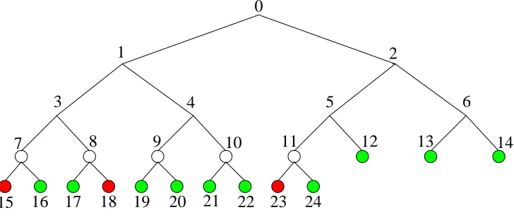
Figure 1: The non-full complete tree T0 withn= 13 users as its leaves. Privileged users are indicated in green and the revoked users are indicated in red. Here, r = 3. The tree T1 is a subtree of T0 and is a full subtree having 8 leaf nodes whereas the tree T2 is a non-full complete subtree ofT0 with 5 leaf nodes.
note here that a complete binary tree has leaf nodes only at the bottom-most or last level and maybe also the last-but-one level. The leaves in the last level are filled from the left to the right in the tree. In a full binary tree of heightℓthere are 2ℓ leaves, all at the last level. A full binary tree is also complete by definition. We will refer to trees that are complete but not full as non-full. Each user inN is associated with a leaf of the complete binary tree T0. There are a total of 2n−1 nodes in T0. The root node of T0 is labeled as 0. All subsequent nodes are labeled as follows: the left child node of a node iis labeled as 2i+ 1 and the right child is labeled as 2i+ 2. Hence, nodes 0 ton−2 are the internal nodes and nodes n−1 to 2n−2 are the leaf nodes. The subtree of T0 rooted at node i is denoted by Ti. The number of leaf nodes in the subtree Ti is denoted by λ
i. The
collection S of subsets is defined as follows: The setSi,j is defined to contain users in the subtreeTi butnot in
Tj. A set S
i,j is also denoted as Ti\ Tj. All subsets of users of the form Si,j, where node j is in the subtreeTi
3 THE COMPLETE TREE SUBSET DIFFERENCE METHOD 6
Once this collectionS has been created, each setSi,j inS has to be assigned a long-lived keyLi,j. We will look
at the key assignment in Section 3.1.
6
8 9 10
7 12 13 14
5 4
3
0
15 16 17 18 19 20 21 22 23 24
1 2
[image:6.612.117.488.133.288.2]11
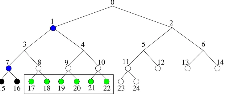
Figure 2: The subset difference subset S1,7 which includes leaves in T1 but not in T7 i.e.; S1,7 = T1\ T7 = {17,18,19,20,21,22}.
During broadcast, the centre will know the setRof revoked users and the messageM to be broadcast. It has to find the subset coverScforN \R. Sccontains pairwise disjoint setsSi1,j1, . . . , Sih,jhsuch thatN \ R=
Sh
k=1Sik,jk where each Sik,jk is taken from S. If the setR is empty, then the only set in the coverSc isN. Otherwise, the following cover-finding algorithm is used: The centre first constructs the Steiner Tree ST(R) induced byR on T0. The Steiner TreeST(R) is a subgraph of T0 that only retains the nodes and edges on paths from the root node 0 to a revoked leaf node. All the other paths inT0 are deleted. The cover-finding algorithm runs iteratively by maintaining a treeT that is a sub-graph ofST(R). It starts by initializing T as a copy ofST(R). At every iteration, the algorithm keeps removing nodes fromT while adding subsets toSc, untilT has just one node left.
At any point of time in the algorithm, a leaf node in T corresponds to either a leaf node in T0 or the root of a subtree in T0 all whose leaves have already been covered till that iteration. More precisely:
1. If there is only one leaf node in T, jump to step 6.
2. Find two leaves j1 and j2 of T whose first common ancestor i does not have any other leaf node in its subtree in T. Here, out of the many possible such pairs j1 and j2 one may choose the leftmost to have a specific algorithm.
3. Let i1 (respectively i2) be the immediate child node of i which is an ancestor of j1 (respectively j2) or is the node j1 (respectively j2) itself. If i1 6=j1 then add the set Si1,j1 to the cover Sc. Similarly, if i2 6= j2
then add the set Si2,j2 to the coverSc.
4. Delete the paths joining j1 and j2 with their common ancestor i. Hence, node ibecomes a leaf inT.
5. If there are more than one leaves remaining inT, go back to step 2.
6. If the only leaf node is the node 0, then there are no more subsets to be added toSc. Else, add the setS0,j
3 THE COMPLETE TREE SUBSET DIFFERENCE METHOD 7
3.1 Key assignment to each subset Si,j in S
Pseudo-random generatorG: In order to assign keys to each subset inS, the centre assigns uniform random seeds to every non-leaf node in T0 and uses a cryptographic pseudo-random generator G. The pseudo-random generatorGoutputs a pseudo-random string that has three times the length of the input seed. The output string
G(seed) is divided into three equal parts GL(seed), GM(seed) and GR(seed). Hence, G(seed) = GL(seed) k
GM(seed)kGR(seed). G:{0,1}k→ {0,1}3k is a pseudo-random generator if no polynomial time adversary can
distinguish between its output for a random seed from a truly random string of the same length.
Seed assignment to nodes: Every non-leaf node iinT0 is assigned a uniform random seedLABELi. Each
non-root node j of T0 is assigned derived seeds from every ancestor i of j. The left child 2i+ 1 of node i in T0 derives the seed G
L(LABELi) from the random seed LABELi of i. All descendants of 2i+ 1 further get
derived seeds from this derived seed GL(LABELi) of 2i+ 1. Similarly, the right child 2i+ 2 of node i in T0
derives the seed GR(LABELi) from the random seed of iand all descendants of 2i+ 2 get derived seeds from
this derived seedGR(LABELi) of 2i+ 2. We denote the seed for a nodejderived from the random seed of node
i asLABELi,j. Following such an assignment of random and derived seeds for nodes in T0, the long lived key
Li,j assigned to the set Si,j isGM(LABELi,j).
Iu for each u∈ N: Once the centre is done with the assignment of random and derived seeds to nodes, it has
to distribute the secret informationIu to each useru∈ N. The user associated with a leafjofT0must have been
revoked when a setSi,j is in the coverSc. Hence, the user at leafjshould not be able to compute theLi,j for any
of its predecessoriinT0. In fact, it should not be able to compute anyL
i,k wherek, a descendant ofi, is also one
of its ancestors. In other words, a user at leafj should be able to compute anLi,k if and only ifiis an ancestor
of j and kbeing a descendant of i, is not on the path joining j withi. In a subtreeTi ofT0 to which a user at leafj belongs, the node ihas a random seed LABELi. The user atj gets the seeds of all nodes adjacent to the
path joiningiandj that have been derived fromLABELi. Sayi1, . . . , im are those nodes “falling off” from the
path between nodeiand leafj. The user atjwill get the derived seedsLABELi,i1, LABELi,i2, . . . , LABELi,im. To summarize, the Iu for a useru at leaf j consists of all derived seeds LABELi,k such that iis a predecessor
of j and k is adjacent to the path joiningiand j. As derived in [NNL01], the number of derived seeds in Iu is
1
2log2n+12logn+ 1 forna power of two. For an arbitraryn, one has to consider the next higher power of two, say 2ℓ0−1 < n≤2ℓ0. The number of derived seeds inI
u will be 12ℓ20+12ℓ0+ 1.
3.2 Dummy Users and the Associated Penalty
The CTSD scheme works with the actual number of users that are present in the system. It may be argued that even ifn is not a power of two, the SD scheme can be applied by incorporating dummy users to make the total number of users to be a power of two. We argue that this impacts the size of the transmission overhead. For an actual broadcast, there are two ways to handle the dummy users – either consider all of them to be revoked or consider all of them to be privileged.
Suppose that the dummy users are considered to be distributed randomly among all the users. Then viewing them as revoked has very serious performance penalties. This is because, the average header length is linear in the number of revoked users, as is proved later. Having a larger number of randomly distributed revoked users leads to larger header size. If, on the other hand, the dummy users are viewed as privileged, then the performance penalty will be lesser.
Assuming the dummy users to be randomly distributed may not be fully justifiable. In an actual imple-mentation, they may be considered to be one block. Suppose that 2ℓ−1 < n <2ℓ and that the users numbered
3 THE COMPLETE TREE SUBSET DIFFERENCE METHOD 8
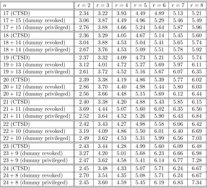
[image:8.612.94.503.89.461.2]n r= 2 r= 3 r = 4 r= 5 r= 6 r= 7 r = 8 17 (CTSD) 2.34 3.22 3.93 4.49 4.89 5.13 5.21 17 + 15 (dummy revoked) 3.06 3.87 4.49 4.96 5.29 5.46 5.49 17 + 15 (dummy privileged) 2.76 3.88 4.66 5.24 5.64 5.87 5.96 18 (CTSD) 2.36 3.29 4.05 4.67 5.14 5.45 5.60 18 + 14 (dummy revoked) 3.04 3.88 4.53 5.04 5.41 5.65 5.74 18 + 14 (dummy privileged) 2.67 3.76 4.53 5.09 5.51 5.78 5.92 19 (CTSD) 2.37 3.32 4.09 4.73 5.21 5.55 5.74 19 + 13 (dummy revoked) 3.12 4.01 4.72 5.27 5.69 5.97 6.11 19 + 13 (dummy privileged) 2.61 3.72 4.52 5.16 5.67 6.07 6.35 20 (CTSD) 2.39 3.38 4.19 4.86 5.39 5.77 6.02 20 + 12 (dummy revoked) 2.86 3.70 4.40 4.98 5.44 5.80 6.03 20 + 12 (dummy privileged) 2.56 3.66 4.48 5.15 5.69 6.12 6.44 21 (CTSD) 2.40 3.38 4.20 4.88 5.43 5.85 6.15 21 + 11 (dummy revoked) 3.69 4.44 5.07 5.60 6.02 6.35 6.56 21 + 11 (dummy privileged) 2.52 3.64 4.52 5.26 5.90 6.43 6.84 22 (CTSD) 2.42 3.43 4.27 4.98 5.58 6.06 6.42 22 + 10 (dummy revoked) 3.19 4.09 4.86 5.50 6.01 6.40 6.69 22 + 10 (dummy privileged) 2.49 3.62 4.53 5.31 5.99 6.56 7.03 23 (CTSD) 2.43 3.44 4.28 4.99 5.60 6.09 6.48 23 + 9 (dummy revoked) 3.27 4.20 5.01 5.68 6.23 6.66 6.98 23 + 9 (dummy privileged) 2.47 3.62 4.58 5.41 6.14 6.77 7.28 24 (CTSD) 2.45 3.48 4.33 5.07 5.71 6.24 6.67 24 + 8 (dummy revoked) 2.70 3.54 4.35 5.08 5.71 6.24 6.67 24 + 8 (dummy privileged) 2.45 3.60 4.59 5.45 6.19 6.83 7.34
Table 1: Comparison of the expected header lengths for 17≤n≤24 and 2≤r≤8 in the CTSD method with the SD method working with dummy users forming a block at the right end. The dummy users may be privileged or revoked. It shows that the CTSD scheme always requires lesser bandwidth than the SD scheme with dummy users.
among the values 1 ton, whereas the users numbered n+ 1, . . . ,2ℓ will be considered to be either all revoked or
all privileged.
4 COMBINATORIAL ANALYSIS OF THE SD AND CTSD METHODS 9
4
Combinatorial Analysis of the SD and CTSD methods
A given set of revoked users is called arevocation pattern. We denote a revocation pattern on n users where
r are revoked, as an (n, r)-revocation pattern. The number of possible (n, r)-revocation patterns is nr
. In order to study the detailed combinatorial behaviour of the CTSD and hence the SD algorithm, we find a method to count the number of (n, r)-revocation patterns that result in a header length ofh.
Definition 1. In a subtree Tj of T0 with λ
j users, N(λj, r, h) is defined as the number of (λj, r)-revocation
patterns that are covered by exactly h subsets. Similarly, for λj users in Tj, T(λj, r, h) is defined as the number
of (λj, r)-revocation patterns that are covered by h subsets such that there is at least one revoked user in both
subtrees of Tj.
Since the tree T0 has n (= λ
0) leaves, N(n, r, h) = N(λ0, r, h) is the number of (n, r)-revocation patterns covered by a header length of h. We obtain recurrences for N(n, r, h).
4.1 Some Notation
Level number and position of nodes: Before we start deriving the expressions forT(n, r, h) andN(n, r, h), we fix a few notation for the ease of description. A level number of T0 is indicated byℓ. In particular, the level of a nodeiis denoted byℓi. The root node 0 is at the highest levelℓ0. Hence,ℓ∈ {0, . . . , ℓ0}. Since every subtree Ti is a complete binary tree, 2ℓi−1 < λ
i ≤2ℓi. The number of nodes at levelℓ of T0 is denoted by qℓ. We see
that the number of nodes at the last level is q0 = 2(n−2ℓ1). For ℓ∈ {1, . . . , ℓ0},qℓ = 2ℓ0−ℓ. The position of a
node at a level from the left is denoted bykwherekranges from 1 toqℓ. Hence, a node iis uniquely represented
by the pair (ℓi, ki) – the level ℓi of T0 to which it belongs and its position ki from the left at that level. As an
example, the root node 0 ofT0 is represented by (ℓ
0,1). We will interchangeably use bothiand (ℓi, ki) to denote
a node.
1 2
6
10
7 14
5 4
3
15 16 17 18 19 20 21 22 23 24
11 12 13
9 8
0
l=1
l=0 l=4
l=3
[image:9.612.99.497.440.591.2]l=2
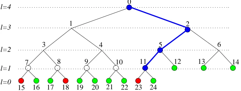
Figure 3: Level numbers in T0. The path P0 is marked with blue. Nodes coloured blue are at position kP ℓ for
the respective level ℓ.
4 COMBINATORIAL ANALYSIS OF THE SD AND CTSD METHODS 10
denoted bykP
ℓ . Letj be a node onP0, say the node represented by (ℓ, kℓP). The part of the pathP0 lying in the
subtree Tj is denoted as P
j. For the level ℓ, the subtreeTj rooted at node (ℓ, kPℓ ) is the only possibly non-full
subtree rooted at level ℓ. The subtrees to the left and right of nodekP
ℓ at levelℓare all full. The subtrees to the
left (respectively right) of node kP
ℓ of level ℓhave 2ℓ (respectively 2ℓ
−1) leaves. The number of leaves in the only
possibly non-full subtree rooted at levelℓis denoted byλℓ,P. The root node of this subtree would be node (ℓ, kP ℓ )
of level ℓ. Hence, 2ℓ−1 < λℓ,P ≤2ℓ. More specifically,λℓ,P =n−((kP
ℓ −1)×2ℓ)−((2ℓ0−ℓ−kℓP)×2ℓ−1). Also,
kP
ℓ =
q0
2ℓ
. We definekPj
ℓ for the pathPj as the position of the node at levelℓonPj from the left in the subtree
Tj. Hence,kP
ℓ is also denoted ask P0
ℓ . One can see thatk Pj
ℓ =
&
q0−(kP
ℓj−1)×(2ℓj) 2ℓ
' =q0
2ℓ
−(kP
ℓj−1)×(2
ℓj−ℓ).
4.2 Recurrences N(n, r, h) and T(n, r, h)
Theorem 1. For a subtreeTi of T0 withλ
i (2ℓ < λi≤2ℓ+1) leaves,
N(λi, r1, h1) =T(λi, r1, h1) + X
j∈IN(i)
T(λj, r1, h1−1) (1)
where IN(i) is the set of all internal nodes in the subtreeTi excluding the node i.
Proof. We show that a revocation pattern is counted inN(λi, r1, h1) if and only if it is counted in exactly one of
T(λi, r, h) orT(λj, r, h−1) for somej ∈IN(i). First we consider a (λi, r)-revocation pattern that is counted in
N(λi, r, h). There exists a minimal subtreeTj, withj∈IN(i), of Ti that contains all the revoked leaves. If this
subtree is rooted at iitself, then that revocation pattern is counted inT(λi, r, h) and is covered by hsubsets of
S. For any other nodej 6=i, the revocation pattern is counted inT(λj, r, h−1) and has to be covered byh−1
subsets of S. The rest of theλi−λj privileged users form one SD subset of the cover. The total cover size will
hence be h. Since a setRof revoked users has a corresponding unique minimal subtree Tj of Ti containing all
the users in R, hence it is counted exactly once on the right side of (1).
Now, let us consider a (λi, r)-revocation pattern that has been counted in T(λi, r, h). By the definitions of
T and N, the (λi, r)-revocation patterns that are counted in T(λi, r, h) are also counted inN(λi, r, h). For some
other revocation pattern, counted in T(λj, r, h−1) for some j∈IN(i), both subtrees ofTj contain at least one
revoked user in each. Hence, the minimal subtree of Ti containing the r revoked users for such a revocation
pattern isTj. For the revocation patterns counted in T(λ
j, r, h−1), the privileged users of the subtreeTj have
been covered withh−1 SD subsets of S. The rest of the λi−λj users are all privileged and are covered by one
more SD subsetSi,j. Hence, the corresponding (λi, r)-revocation pattern is counted in N(λi, r, h).
Theorem 2. For a subtreeTi of T0 withλ
i (2ℓ < λi≤2ℓ+1) leaves,
T(λi, r1, h1) =
r1−1
X
r′=1
h1
X
h′=0
N(λ2i+1, r′, h′)×N(λ2i+2, r1−r′, h1−h′) (2)
where λ2i+1 (respectively λ2i+2) is the number of leaves in the left (respectively right) subtree of Ti.
Proof. We show that a revocation pattern is counted in T(λi, r1, h1) if and only if it is counted in the right hand side of (2). For a given λi, the number of leaves in the left and right subtrees get fixed to λ2i+1 and
λ2i+2 respectively. When a (λi, r1)-revocation pattern is counted in T(λi, r1, h1), both the subtrees of Ti must have at least one revoked user. Assuming the left subtree of Ti has r′ revoked users, the right subtree should
have r1−r′ revoked users since the total number of revoked users isr1. Similarly, assuming that the privileged users in this left subtree are covered by h′ sets of S, the privileged users in the right subtree should be covered
4 COMBINATORIAL ANALYSIS OF THE SD AND CTSD METHODS 11
T(λi, r1, h1) r1<0 r1 = 0 r1= 1 2≤r1 < n r1 =n r1 > n
h1= 0 0 0 0 0 1 0
h1≥1 0 0 0 from (2) 0 0
N(λi, r1, h1) r1<0 r1 = 0 r1= 1 2≤r1 < n r1 =n r1 > n
h1= 0 0 0 0 0 1 0
h1= 1 0 1 n from (1) 0 0
[image:11.612.125.472.89.199.2]h1>1 0 0 0 from (1) 0 0
Table 2: Boundary conditions on T(n, r, h) andN(n, r, h).
is N(λ2i+1, r′, h′). Similarly, the number of (λ2i+2, r1 −r′)-revocation patterns in the right subtree covered by
h1−h′ subsets isN(λ2i+2, r1−r′, h1−h′). Each such (λ2i+1, r′)-revocation pattern in the left subtree along with a (λ2i+2, r1−r′)-revocation pattern in the right subtree gives rise to a (λi, r)-revocation pattern in the treeTi
that is covered byh1 subsets ofS. Hence, for all values of r′ ∈ {1, . . . , r1−1} and all values of h′ ∈ {0, . . . , h1},
N(λ2i+1, r′, h′)×N(λ2i+2, r1−r′, h1−h′) counts all the possible T(λi, r1, h1).
Any (λi, r1)-revocation pattern covered by h′ subsets will be counted in someN(λ2i+1, r′, h′)×N(λ2i+2, r1−
r′, h
1−h′). The ones counted inN(λ2i+1, r′, h′)×N(λ2i+2, r1−r′, h1−h′) for fixed values ofr′andh′ are counted exactly once in it. For other values of r′ and h′, the corresponding (λ
i, r1)-revocation patterns will be counted in the respective N(λ2i+1, r′, h′)×N(λ2i+2, r1−r′, h1−h′). Hence, a (λi, r1)-revocation pattern is counted on the right hand side of (2) if and only if it is counted in T(λi, r1, h1).
Boundary conditions: The boundary conditions onT(λi, r1, h1) andN(λi, r1, h1) are given in Table 2. Other than the tabulated values, N(λi, r1, h1) = 0 for λi ≤ 0 and T(λi, r1, h1) = 0 for λi ≤ 1. From recurrences in
Theorems 1 and 2 and the boundary conditions on these recurrences, one can find the value ofN(n, r, h) for any given n,r and h using dynamic programming.
4.3 Algorithms to compute N(n, r, h) and T(n, r, h)
Substituting for j ∈ IN(i): To use these recurrences as an algorithm, the nodes j ∈ IN(i) in (1) for a node
i have to be explicitly identified and the corresponding λjs have to be substituted. As described in Section 4.1
before, there are at most three types of subtrees rooted at a levelℓj ofT0: full subtrees of heightℓi, full subtrees
of heightℓi−1 and a non-full complete subtree of heightℓi.
(1) For a subtree Ti that is full and is of height 2ℓi and to the left of the node at positionkP
ℓi at level ℓi:
N(λi, r1, h1) =T(λi, r1, h1) +
ℓi−1 X
ℓj=1
(2ℓi−ℓj)×T(2ℓj, r
1, h1−1). (3)
(2) For a subtree Ti that is full and is of height 2ℓi−1 and to the right of the node at positionkP
ℓi at level ℓi:
N(λi, r1, h1) =T(λi, r1, h1) +
ℓi−1 X
ℓj=2
(2ℓi−ℓj)×T(2ℓj−1, r
4 COMBINATORIAL ANALYSIS OF THE SD AND CTSD METHODS 12
(3) For the only possibly non-full subtree Ti fori= (ℓ
i, kPℓi) of height 2ℓi and at position kℓPi at levelℓi:
N(λi, r1, h1) =T(λi, r1, h1)
+
ℓi−1 X
ℓj=2 [(kPi
ℓj −1)×T(2
ℓj, r
1, h1−1) +T(λℓj,P, r1, h1−1)
+ (2ℓi−ℓj−kPi
ℓj)×T(2
ℓj−1, r
1, h1−1)]. (5)
Dynamic Programming: ComputingN(n, r, h) andT(n, r, h) requires computing the values of N(λi, r1, h1) and T(λi, r1, h1) for some smaller λi, r1 and h1. We use dynamic programming technique where all values of
N(λi, r1, h1) andT(λi, r1, h1) for smaller λi,r1 and h1 are pre-computed. The algorithm to compute T(n, r, h) from these pre-computed values is obtained from (2) in a straightforward manner. The algorithm to compute
N(n, r, h) from these pre-computed values is obtained from (1). More specifically from either of (3) or (5). Level
ℓi ofT0 haskPℓi−1 full subtrees of heightℓi, (2
ℓ0−ℓi)−kP
ℓi full subtrees of heightℓi−1 and one possibly non-full subtree. For every level in the treeT0, T(λi, r, h−1) is pre-computed once for each of the three types of nodes
and used to compute N(n, r, h).
Space and Time complexity of the algorithm: Using (2) to compute T(n, r, h) from the pre-computed values of N(·,·,·) requires O(rh) memory operations and multiplications. Equation (1) shows how N(n, r, h) is related to pre-computed values of T(·,·,·). Actual computation is done using (3), (4) and (5). This requires
O(1) memory operations and a single addition for each of the ⌈logn⌉ levels of T0. Hence, the time complexity for computing T(n, r, h) and then N(n, r, h) from pre-computed valuesisO(rh+ logn).
These pre-computed values in turn need to be computed. By the form of (3), (4) and (5) there are logn
subtrees to be considered. For each such subtree,O(rh) values need to be computed and the computation of these will be based on values computed earlier. A dynamic programming algorithm proceeds in a bottom-up fashion by computing the O(rh) values corresponding to smaller sub-trees and then using these to compute the values for progressively larger sub-trees. This takes a total of O(r2h2logn+rhlog2n) time. The space requirement is given by the number of pre-computed values that need to be stored to compute N(n, r, h). For each of the
O(logn) sub-trees, a total ofO(rh) values need to be stored and so the space complexity isO(rhlogn).
The above time and space complexities are required for a single set of values ofn,rand h. For a fixednand
r, it may be required to compute the values of N(n, r, h) for all possible values of h. This would be a typical requirement for a broadcast centre which will have a fixed number of users and for a particular transmission knows the number of revoked users. The corresponding time and space complexities can be obtained by substituting an appropriate value for h. In Lemma 9 in Appendix A, we show that h ≤ 2r−1 which gives the expressions
O(r4logn+r2logn) and O(r2log2n) for time and space complexities respectively. For large n and moderate values of r, these are practical complexities.
Further, allowing r to range over all the O(n) possible values leads to O(n4logn+n2log2n) time and
O(n2logn) space complexities respectively. If we are interested in computingN(i, r, h) for all 2≤i≤nand all possible values of r and h, then the time and space complexities areO(n5+n3logn) and O(n3) respectively.
As an example, using this dynamic programming algorithm, we find that for n = 126, r = 63 and h = 37, the floating point value ofN(n, r, h) is 7.44×1035. Note that computing such a value would not be possible by direct enumeration. Attempting direct enumeration, would require considering 12663
4 COMBINATORIAL ANALYSIS OF THE SD AND CTSD METHODS 13
4.4 Upper Bounds on the Header Length
The header length is an important efficiency parameter of a broadcast encryption scheme. So, upper bounds on the header length of the SD and CTSD schemes are of practical interest. A detailed combinatorial analysis of upper bounds on the header length is given in Appendix A. Here, we present a summary of the important results. The proofs are given in Appendix A.
In Lemma 9 in Appendix A, it is shown that the header length of the CTSD scheme is at most 2r−1. For the special case of the SD method, this bound was proved in [NNL01]. This bound is made more specific in Theorem 3 below for the CTSD and hence the SD method.
Theorem 3. The maximum header length in the CTSD method for n users is min(2r−1,n 2
, n−r).
The bound given by Theorem 3 gives a complete picture. Ifr≤n/4, then the bound 2r−1 is appropriate; ifn/4< r≤n/2, then the bound ⌊n/2⌋ is appropriate; and for r > n/2, the bound (n−r) is appropriate. The last bound has an important consequence. If the number of revoked users is greater than n/2, it may appear that using individual transmission to the privileged users would be better than using the CTSD method. But, The bound of (n−r) on the header size shows that this is not true. Using the CTSD method is never worse than individual transmission to privileged users.
The bound of Theorem 3 holds for the SD scheme, i.e., for full trees. The only previously proved upper bound for the SD scheme is 2r−1. The other two bounds do not appear to have been reported with proofs in the literature. In fact, there does not seem to be an easy way to argue about these bounds without using the recurrences that we have derived.
Fix a value forr and denote bynr the minimum value ofnsuch that there exists an (n, r)-revocation pattern
giving rise to a header of size 2r−1. Theorem 4 characterizes nr.
Theorem 4. In the CTSD method, let 2k−1 < r≤2k. When r ≤2k−1+ 2k−2, let r1 = 2k−2 and r0 =r−2k−2
and hence,
nr=nr0+ 2
2k−2+ 22k−1
and when r >2k−1+ 2k−2, letr0= 2k−1 andr1 =r−2k−1 and hence,
nr = 22k−1+nr1 + 2
2k−1.
From this it easily follows that for the SD method, for any r in the range 2k−1 < r ≤2k,n
r = 22k+1. This
has been earlier proved in [MMW09].
For the SD scheme the number of users is a power of 2. In this case, we show that the recurrences lead to a generating function for the sequence N(n, r, h). Let the number of users ben= 2ℓ0 and hence the treeT0 is full
and of heightℓ0. For a full tree T0, all subtreesTi are full and at levelℓ, there are 2ℓ0−ℓ subtrees with 2ℓ leaves in each.
We defineTℓ(r, h) =T(2ℓ, r, h) and Nℓ(r, h) =N(2ℓ, r, h). Then the recurrences (1) and (2) for counting the
number of revocation patterns become.
Nℓ0(r, h) =Tℓ0(r, h) +
ℓ0−1
X
ℓ=1
2ℓ0−ℓ
×Tℓ(r, h−1)
. (6)
Tℓ0(r, h) =
r−1 X
r1=1
h
X
h1=0
Nℓ0−1(r1, h1)×Nℓ0−1(r−r1, h−h1). (7)
5 EXPECTED HEADER LENGTH IN THE CTSD AND SD METHODS 14
Theorem 5. The generating function for the sequence Nℓ0(r, h) of numbers defined in (6) above, is given by
Xℓ0(x, y) where
Xℓ0(x, y) =
Xℓ0−1(x, y)−xy
2ℓ0−12
+xy2ℓ0
+ 2ℓ0
x2y2ℓ0−1
+
ℓ0−1
X
ℓ=1
2ℓ0−ℓ
xy2ℓ0−2ℓ
×Xℓ−1(x, y)−xy2 ℓ−12
.
A similar generating function was found by Park and Blake in [PB06]. It was directly derived based on the structural properties of the tree. We have taken a different approach of first finding the recurrence relations for the sequenceN(n, r, h) and then deriving the generating function from it.
5
Expected Header Length in the CTSD and SD methods
In the previous section, we have studied upper bounds on the header length. In practice, however, it is of interest to know the average header length. This will provide a broadcast centre with valuable information about the average communication bandwidth.
Given the number of users n such that 2ℓ0−1 < n≤ 2ℓ0, and the number of revoked users r, there are n
r
possible revocation patterns. Each such revocation pattern gives rise to a subset cover for the privileged users and hence a header in the ciphertextC. We now obtain an algorithm to compute the expected header length for a given nand r in the CTSD scheme. In particular this algorithm applies to the SD method and is of significant practical interest.
The Random Experiment: We consider the random experiment where r out of the n initially un-revoked leaves of the tree T0 are chosen uniformly at random without replacement and revoked. This gives rise to a random (n, r)-revocation pattern and hence a corresponding random subset cover Sc and its header length h.
Let Xn,r be the random variable taking the value of the header length h due to the (n, r)-revocation pattern of
the above experiment. Next, we associate a random variable with each node of the tree T0. Let Xn,ri ∈ {0,1} be a random variable associated with node iof T0. Xi
n,r = 1 denotes the event that the cover contains a subset
Si,j = Ti\ Tj where j is some node in the subtree Ti. In other words, when Xn,ri = 1 we say that node i
generates a subset for the cover. Similarly, Xn,ri = 0 denotes the event that there is no subset Si,j in the cover.
Since i is also represented by (ℓi, ki), Xn,ri will also be written asXn,rℓi,ki whenever the nodes need to be viewed
level-wise and is appropriate in the context.
The Expected Header Length: Since the header constitutes of subsets Si,j, each rooted at a different node
i, it is easy to see that,Xn,r=Xn,r0 +Xn,r1 +. . .+Xn,rn−2. By linearity of expectation:
E[Xn,r] =E[Xn,r0 ] +E[Xn,r1 ] +. . .+E[Xn,rn−2]. (8)
Since all the random variables Xt
n,r follow a Bernoulli distribution with probabilityPr[Xn,rt = 1], we get:
E[Xn,r] = Pr[Xn,r0 = 1] + Pr[Xn,r1 = 1] +. . .+ Pr[Xn,rn−2 = 1]. (9)
Calculating each of these n−1 probability terms individually would give the expected header length. However, the running time can be optimized. Recall thatP0 is the unique path from the root to a leaf node which contains the nodes at which the non-full subtrees ofT0 are rooted. As we had discussed before, the subtreesTifor which
i is not on P0 are full. For a level ℓ of T0 the subtrees to the left of P0 are all full and have equal number of leaves. Hence, Pr[Xi
n,r = 1] needs to be computed only once for every such node i to the left of P0 at level ℓ.
Similarly for nodes to the right of P0. Hence, efficient computation of E[X
5 EXPECTED HEADER LENGTH IN THE CTSD AND SD METHODS 15
Pr[Xn,rj = 1] level-wise. There are qℓ internal nodes at all levels ℓ ≥ 2. At level 1, there are n−2ℓ1 = q0/2 internal nodes. The otherq1−(n−2ℓ1) nodes at level 1 are leaves. Hence, (9) can also be written as:
E[Xn,r] = ℓ0
X
ℓ=2
qℓ X
k=1
Pr[Xn,rℓ,k = 1] +
q0/2
X
k=1
Pr[Xn,r1,k = 1]. (10)
When r= 0, there is only one setN in the coverSc and hence, E[Xn,0] = 1. Here on, we will considerr ≥1.
Pr[Xℓi,ki
n,r = 1] for the node i of Ti: The sibling subtree Ts of node i may be Ti−1 on its left or Ti+1 on
its right. To find the probability that node i generates a subset Si,j for the cover, we observe that the event
Xn,ri = 1 occurs when the sibling subtreeTs of ihas at least one revoked node and exactly one of the subtrees of ihas at least one revoked user. We define the events Ri
sb,Rilt and Rirt for node iwith respect to our random
experiment. Risb denotes the event that the number of revoked nodes in the sibling subtree of Ti is non-zero.
Rilt(respectivelyRrti ) denotes the event that the number of revoked nodes in the left (respectively right) subtree T2i+1 (respectively T2i+2) is non-zero.
lt rt sb
i
2i+1 2i+2
sb
i
2i+1 2i+2
rt
[image:15.612.40.560.310.429.2]lt
Figure 4: Figures demonstrating the eventsRisb∧Rirt∧Ri
ltandRisb∧Rilt∧Rirtrespectively. The triangles represent
subtrees rooted at the respective nodes. White denotes that the subtree has no revoked user in it. Gray denotes that the subtree has at least one revoked user in it. The sizes of the subtrees are not to the scale of the number of users in them.
Lemma 6. For an internal non-root node i in T0, the probability that the cover S
c contains a set of the form
Ti\ Tj where j is some node in the subtree Ti, is given byPr[Xn,ri = 1] where
Pr[Xn,ri = 1] = Pr[Risb∧Rirt∧Rlti] + Pr[Risb∧Rilt∧Rirt].
For the root node 0, this probability is given byPr[Xn,r0 = 1]where
Pr[Xn,r0 = 1] = Pr[R0
lt] + Pr[R0rt].
Proof. For a non-root node i, a subset Si,j occurs in the cover when there is at least one revoked user in exactly
one of the subtreesT2i+1 orT2i+2 ofi. The sibling subtreeTsshould also have at least one revoked user. Hence
the event Xn,ri = 1 can be divided into two mutually exclusive and exhaustive events. First, when the sibling subtree and the right subtree ofTi have at least one revoked user in each and the left subtree does not have any:
(Risb∧Rirt∧Rilt). Second, when the sibling subtree and the left subtree ofTi have at least one revoked user in
each and the right subtree does not have any: (Ri
sb∧Rlti ∧Rirt).
5 EXPECTED HEADER LENGTH IN THE CTSD AND SD METHODS 16
To simplify the computation of these probabilities in Lemma 6, we define a new notationηr(α, β) to indicate
the probability of choosing r elements from a set of α elements such that β out of these α elements are never chosen. So, ifβ ≥α−r+ 1, then ηr(α, β) = 0 by definition. Else, for 0< β < α−r+ 1,
ηr(α, β) = α−β
r
α r
=
1−β
α 1− β
α−1 1−
β α−2
. . .
1− β
α−r+ 1
. (11)
Theorem 7. For an internal non-root node i of T0 whose sibling subtree hasλ
s leaves,
Pr[Xn,ri = 1] =ηr(n, λ2i+1) +ηr(n, λ2i+2)−ηr(n, λs+λ2i+1)−ηr(n, λs+λ2i+2)
−2ηr(n, λ2i+1+λ2i+2) + 2ηr(n, λs+λ2i+1+λ2i+2). (12)
For the root node 0 of T0,
Pr[Xn,r0 = 1] =ηr(n, λ1) +ηr(n, λ2). (13)
Proof. The following two expressions can be obtained by usual probability arguments.
Pr[Risb∧Rirt∧Rilt] = Pr[Rilt]−Pr[Risb∧Rilt]−Pr[Rirt∧Rilt] + Pr[Risb∧Rirt∧Rilt]; Pr[Risb∧Rilt∧Rirt] = Pr[Rirt]−Pr[Risb∧Rrti ]−Pr[Rilt∧Rirt] + Pr[Risb∧Rilt∧Rirt].
)
(14)
Next, we deduce the expression for finding Pr[Ri
sb ∧Rilt∧Rirt] in terms of ηr(·,·). This is the probability of
choosingr elements from nsuch that none of the users in the subtreesT2i+1,T2i+1 or the sibling subtreeTs of
iare chosen. Consequently, Pr[Ri
sb∧Rilt∧Rirt] =ηr(n, λs+λ2i+1+λ2i+2). The other probabilities on the right hand sides of (14) can be found similarly by excluding the users in the respective subtrees. From Lemma 6, and substituting the probabilities on the right hand sides of (14) with their correspondingηr(·,·) equivalents, we get:
Pr[Xn,ri = 1] =ηr(n, λ2i+1) +ηr(n, λ2i+2)−ηr(n, λs+λ2i+1)−ηr(n, λs+λ2i+2)
−2ηr(n, λ2i+1+λ2i+2) + 2ηr(n, λs+λ2i+1+λ2i+2). (15)
For the root node, Pr[Xn,r0 = 1] = Pr[R0
lt] + Pr[R0rt] where Pr[R0lt] =ηr(n, λ1) and Pr[R0rt] =ηr(n, λ2). Hence,
Pr[Xn,r0 = 1] =ηr(n, λ1) +ηr(n, λ2). (16)
The algorithm for computing E[Xn,r]: Now that we have the expressions to find Pr[Xn,ri = 1] for all
i∈ {0, . . . , n−2} in Theorem 7, the values for λs,λ2i+1 and λ2i+2 for nodei have to substituted appropriately in (15) and (16). By doing these substitutions for nodes at each level ℓ∈ {1, . . . , ℓ0} ofT0, we get the complete algorithm. For level ℓ∈ {2, . . . , ℓ0 −1}, this computation is done in four steps: (1) for the node kPℓ of level ℓ, (2) its sibling subtree, (3) all full subtrees to the left of the above two subtrees, and (4) all full subtrees to the right of the two subtrees in 1 and 2. The subtree at position kP
ℓ at level ℓ is the only possible non-full subtree
for level ℓand is of height ℓ. If kP
ℓ is odd, its sibling subtree is full and of heightℓ−1. IfkPℓ is even, its sibling
subtree is full and of height ℓ. The subtree at node kP
ℓ−1 of level ℓ−1 is always a subtree of the tree rooted at node kP
ℓ of level ℓ. When kℓ−P1 is odd, the right subtree of the tree rooted at node kℓP of level ℓ is full. When
kP
ℓ−1 is even, the left subtree of the tree rooted at nodekPℓ of levelℓ is full. For the root node 0 and the nodes
at level 1, the substitutions are more simple.
To analyze the running time of the algorithm, we observe that each computation of ηr(α, β) involves O(r)
multiplications and there are a constant number of computations of ηr(α, β) for each level of the tree. Hence,
5 EXPECTED HEADER LENGTH IN THE CTSD AND SD METHODS 17
Remarks.
Simulation method for estimating the expected header length: Suppose it is desired to obtain an idea of the average header length for n users of which r are revoked. One can choose k random revocation patterns. For each such pattern, the actual header generation algorithm is executed and the header size is obtained. The average header size over thekpatterns provides an idea of the average header length. This method, however, is less efficient than our algorithm to compute the expected header length. For each of thekrevocation patterns, the simulation will have to construct the Steiner Tree to compute the generated subsets. Each such run will require Ω(r2logn) memory accesses and O(n) space for finding the cover and hence the header length. In comparison, our algorithm requiresO(rlogn) multiplications and O(1) space and finds the exact header length. Further, it is much simpler to implement.
On the other hand, there is a situation where the simulation method may be useful. For the probability analysis, it is usual to assume that revocations take place uniformly. In practice, though, this may not be true. For non-uniform distributions, mathematical analysis may not be possible. For such situations, there is no other option but to use the simulation method to get an idea of the average header length. Additionally, simulations may provide more information about the probability distribution than just the average header length.
Approximation: In [PB06] a formula is given for the expected header length. However, they mentioned that their equations were “complex to compute and difficult to gain insight from”. Consequently, they went forward to find approximationsfor the same. In contrast, our algorithm computes the exact value of the expected header length. Also, [PB06] work only with the SD scheme and so their results do not apply when the number of users is not a power of two.
We have implemented our algorithm to compute the expected header length. Table 3 shows that asr goes above a certain minimum, the expected header length of the CTSD method is significantly better than the SD method. To summarize, the CTSD algorithm always gives better transmission efficiency and its cumulative improvement over many messages is significant on the bandwidth. Since replacing the SD algorithm with the CTSD scheme can be done with very little additional cost the CTSD algorithm should be the more efficient and practical choice.
5.1 Asymptotic Analysis of the Expected Header Length for the SD Method
It is of interest to find the maximum possible value of the expected header length. We carry out this task for full binary trees. In this case, the CTSD method becomes the SD method.
For n= 2ℓ0, for any internal node i∈ {0, . . . , n−2}, λ
2i+1 = λ2i+2 = 2ℓi−1. For any node at level ℓi > 0,
λs= 2ℓi+1. Substituting these values for a node (ℓ, k), (15) becomes:
Pr[Xn,rℓ,k = 1] = 2[ηr(n,2ℓ−1)−ηr(n,2×2ℓ−1)−ηr(n,3×2ℓ−1) +ηr(n,4×2ℓ−1)]. (17)
This probability is independent ofk. In other words, the probability of generating a subset for the cover is equal for all nodes at levelℓ. Define
B(n,rℓ) = Pr[∆ Xn,rℓ,k = 1] = 2[ηr(n,2ℓ−1)−ηr(n,2×2ℓ−1)−ηr(n,3×2ℓ−1) +ηr(n,4×2ℓ−1)]. (18)
Note that by this definition, for the only node at level ℓ0, i.e., the root node, B(ℓ
0)
n,r = 2ηr(n,2ℓ0−1) which is
consistent with (16) forn= 2ℓ0. For a givenn= 2ℓ0 and r, the expected header length H
n,r due to the subset
cover algorithm of the CTSD scheme is defined as:
Hn,r =∆E[Xn,r] = ℓ0
X
ℓ=1
2ℓ0−ℓB(ℓ)
6 CONCLUSION 18
r n <2ℓ0 (CTSD) CTSDE[X
n,r] n= 2ℓ0 (SD) SDE[Xn,r] Extra KBytes
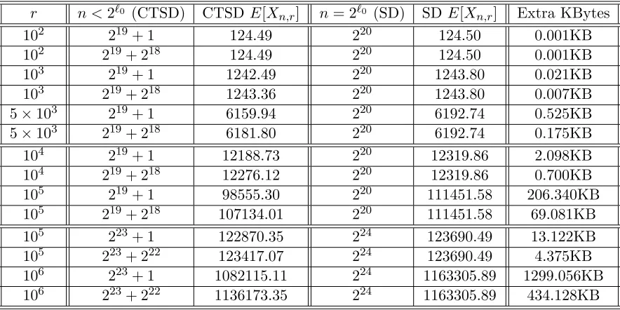
[image:18.612.77.519.90.311.2]102 219+ 1 124.49 220 124.50 0.001KB 102 219+ 218 124.49 220 124.50 0.001KB 103 219+ 1 1242.49 220 1243.80 0.021KB 103 219+ 218 1243.36 220 1243.80 0.007KB 5×10³ 219+ 1 6159.94 220 6192.74 0.525KB 5×10³ 219+ 218 6181.80 220 6192.74 0.175KB 104 219+ 1 12188.73 220 12319.86 2.098KB 104 219+ 218 12276.12 220 12319.86 0.700KB 105 219+ 1 98555.30 220 111451.58 206.340KB 105 219+ 218 107134.01 220 111451.58 69.081KB 105 223+ 1 122870.35 224 123690.49 13.122KB 105 223+ 222 123417.07 224 123690.49 4.375KB 106 223+ 1 1082115.11 224 1163305.89 1299.056KB 106 223+ 222 1136173.35 224 1163305.89 434.128KB
Table 3: The expected header lengths for the SD and CTSD schemes for different n and r and the number of extra bytes needed per message of broadcast. Here we assume each session key is 128 bits long. The additional number of bytes required by the SD scheme is computed as 16 times the difference in header length of the two schemes.
As n increases, the value of Hn,r converges to a limit which depends only on r and is independent of n. The
following result gives this limiting upper bound onHn,r. We use the notationx↑ ato denote that a variablex
increases to the limit a.
Theorem 8. For all n≥1, r ≥1, the expected header length Hn,r ↑Hr, as n increases through powers of two,
where
Hr= 3r−2−3× r−1 X
i=1
−1 2
i +
i
X
k=1 (−1)k
i k
(2k−3k)
(2k−1)
!
.
The proof requires a bit of detailed combinatorial analysis and is provided in Appendix C. We have computed the ratioHr/rfor many values of r and have found it to be always less than 1.25.
In [NNL01], a sketchy argument was given to show that Hn,r is bounded above by 1.38r. It was mentioned
that simulation results showed a tighter upper bound of 1.25r. Values computed using Theorem 8 explain this observation. On the other hand, Theorem 8 shows that the actual limiting value for the expected header length is much more complicated than the simple 1.25r that was suggested in [NNL01]. Our experiments have shown that the convergence to this limiting value is quite fast. Further, the bound given by Theorem 8 can be computed inO(r) time and O(1) space.
6
Conclusion
REFERENCES 19
Detailed combinatorial analysis of the CTSD scheme is done by finding two recurrences to count the number of ways r out ofn users can be revoked to result in a subset cover size of h in the CTSD method. Using these recurrences, it is proved that the maximum possible header length for a given r is 2r−1. This is no worse than the SD scheme even though arbitrary number of users are accommodated. The maximum header length for all
r is n 2
. The recurrences are the most efficient tool as per our knowledge to generate exhaustive data for the above count. Using the recurrences, we also find and prove the expression for the minimum number of users required to be in a system so that for a givenr, the maximum cover size would reach 2r−1. For na power of two, a generating function is found for generating the same sequence as the recurrences.
Probabilistic analysis of the revocation patterns in the CTSD scheme gives the most important result of this work: an efficient algorithm to compute the expected header length for a given nand r. Using this algorithm, it is shown that for practical values of n and r, the CTSD scheme provides better transmission efficiency as compared to the SD scheme. An asymptotic analysis is done using this algorithm that not only gives theoretical support to the empirical upper bound of 1.25r mentioned in [NNL01], but also gives an expression to compute the maximum possible expected header length for a given r in the SD algorithm inO(r) time.
Acknowledgement: We thank the anonymous reviewers for their comments that has helped to improve the paper.
References
[AAC] AACS. Advanced Access Content System, http://www.aacsla.com.
[AK08] Per Austrin and Gunnar Kreitz. Lower bounds for subset cover based broadcast encryption. In Serge Vaudenay, editor,AFRICACRYPT, volume 5023 ofLecture Notes in Computer Science, pages 343–356. Springer, 2008.
[AKI03] Nuttapong Attrapadung, Kazukuni Kobara, and Hideki Imai. Sequential key derivation patterns for broadcast encryption and key predistribution schemes. In Chi-Sung Laih, editor,ASIACRYPT, volume 2894 ofLecture Notes in Computer Science, pages 374–391. Springer, 2003.
[Asa02] Tomoyuki Asano. A revocation scheme with minimal storage at receivers. In Yuliang Zheng, editor,
ASIACRYPT, volume 2501 ofLecture Notes in Computer Science, pages 433–450. Springer, 2002.
[Ber91] Shimshon Berkovits. How to broadcast a secret. In Donald W. Davies, editor,EUROCRYPT, volume 547 ofLecture Notes in Computer Science, pages 535–541. Springer, 1991.
[BF99] Dan Boneh and Matthew K. Franklin. An efficient public key traitor tracing scheme. In Michael J. Wiener, editor, CRYPTO, volume 1666 of Lecture Notes in Computer Science, pages 338–353. Springer, 1999.
[BGW05] Dan Boneh, Craig Gentry, and Brent Waters. Collusion resistant broadcast encryption with short ciphertexts and private keys. In Victor Shoup, editor, CRYPTO, volume 3621 of Lecture Notes in Computer Science, pages 258–275. Springer, 2005.
[BS11] Sanjay Bhattacherjee and Palash Sarkar. An analysis of the Naor-Naor-Lotspiech Subset Difference algorithm (for possibly incomplete binary trees). In Daniel Augot and Anne Canteaut, editors,
Workshop on Coding and Cryptography, April 11-15, 2011, Workshop on Coding and Cryptography, pages 483–492. INRIA, 2011.
REFERENCES 20
[DF03] Yevgeniy Dodis and Nelly Fazio. Public key trace and revoke scheme secure against adaptive chosen ciphertext attack. In Yvo Desmedt, editor, Public Key Cryptography, volume 2567 ofLecture Notes in Computer Science, pages 100–115. Springer, 2003.
[EOPR08] Christopher Eagle, Mohamed Omar, Daniel Panario, and Bruce Richmond. Distribution of the number of encryptions in revocation schemes for stateless receivers. In Uwe Roesler, Jan Spitzmann, and Marie-Christine Ceulemans, editors, Fifth Colloquium on Mathematics and Computer Science, volume AI ofDMTCS Proceedings, pages 195–206. Discrete Mathematics and Theoretical Computer Science, 2008.
[FN93] Amos Fiat and Moni Naor. Broadcast encryption. In Douglas R. Stinson, editor,CRYPTO, volume 773 ofLecture Notes in Computer Science, pages 480–491. Springer, 1993.
[FT01] Amos Fiat and Tamir Tassa. Dynamic traitor tracing. J. Cryptology, 14(3):211–223, 2001.
[GST04] Michael T. Goodrich, Jonathan Z. Sun, and Roberto Tamassia. Efficient tree-based revocation in groups of low-state devices. In Matthew K. Franklin, editor,CRYPTO, volume 3152 ofLecture Notes in Computer Science, pages 511–527. Springer, 2004.
[GW09] Craig Gentry and Brent Waters. Adaptive security in broadcast encryption systems (with short ciphertexts). In Antoine Joux, editor, EUROCRYPT, volume 5479 of Lecture Notes in Computer Science, pages 171–188. Springer, 2009.
[HS02] Dani Halevy and Adi Shamir. The LSD broadcast encryption scheme. In Moti Yung, editor,
CRYPTO, volume 2442 ofLecture Notes in Computer Science, pages 47–60. Springer, 2002.
[JG04] Shaoquan Jiang and Guang Gong. Multi-service oriented broadcast encryption. In Huaxiong Wang, Josef Pieprzyk, and Vijay Varadharajan, editors,ACISP, volume 3108 ofLecture Notes in Computer Science, pages 1–11. Springer, 2004.
[JHC+05] Nam-Su Jho, Jung Yeon Hwang, Jung Hee Cheon, Myung-Hwan Kim, Dong Hoon Lee, and Eun Sun Yoo. One-way chain based broadcast encryption schemes. In Ronald Cramer, editor,EUROCRYPT, volume 3494 ofLecture Notes in Computer Science, pages 559–574. Springer, 2005.
[KY01] Aggelos Kiayias and Moti Yung. Self protecting pirates and black-box traitor tracing. In Joe Kilian, editor, CRYPTO, volume 2139 ofLecture Notes in Computer Science, pages 63–79. Springer, 2001.
[LS98] Michael Luby and Jessica Staddon. Combinatorial bounds for broadcast encryption. In Kaisa Nyberg, editor,EUROCRYPT, volume 1403 ofLecture Notes in Computer Science, pages 512–526. Springer, 1998.
[LT08] Yi-Ru Liu and Wen-Guey Tzeng. Public key broadcast encryption with low number of keys and constant decryption time. In Ronald Cramer, editor, Public Key Cryptography, volume 4939 of
Lecture Notes in Computer Science, pages 380–396. Springer, 2008.
[MMW09] Thomas Martin, Keith M. Martin, and Peter R. Wild. Establishing the broadcast efficiency of the subset difference revocation scheme. Des. Codes Cryptography, 51(3):315–334, 2009.
21
[NP98] Moni Naor and Benny Pinkas. Threshold traitor tracing. In Hugo Krawczyk, editor, CRYPTO, volume 1462 ofLecture Notes in Computer Science, pages 502–517. Springer, 1998.
[PB06] E. C. Park and Ian F. Blake. On the mean number of encryptions for tree-based broadcast encryption schemes. J. Discrete Algorithms, 4(2):215–238, 2006.
[PGM04] Carles Padr´o, Ignacio Gracia, and Sebasti`a Mart´ın Mollev´ı. Improving the trade-off between storage and communication in broadcast encryption schemes. Discrete Applied Mathematics, 143(1-3):213– 220, 2004.
[PGMM02] Carles Padr´o, Ignacio Gracia, Sebasti`a Mart´ın Mollev´ı, and Paz Morillo. Linear key predistribution schemes. Des. Codes Cryptography, 25(3):281–298, 2002.
[PGMM03] Carles Padr´o, Ignacio Gracia, Sebasti`a Mart´ın Mollev´ı, and Paz Morillo. Linear broadcast encryption schemes. Discrete Applied Mathematics, 128(1):223–238, 2003.
[PPS11] Duong Hieu Phan, David Pointcheval, and Mario Strefler. Security notions for broadcast encryption. In Javier Lopez and Gene Tsudik, editors,ACNS, volume 6715 ofLecture Notes in Computer Science, pages 377–394. Springer, 2011.
[SSW01] Alice Silverberg, Jessica Staddon, and Judy L. Walker. Efficient traitor tracing algorithms using list decoding. In Colin Boyd, editor,ASIACRYPT, volume 2248 ofLecture Notes in Computer Science, pages 175–192. Springer, 2001.
[Sti97] Douglas R. Stinson. On some methods for unconditionally secure key distribution and broadcast encryption. Des. Codes Cryptography, 12(3):215–243, 1997.
[SW98] Douglas R. Stinson and Ruizhong Wei. Combinatorial properties and constructions of traceability schemes and frameproof codes. SIAM J. Discrete Math., 11(1):41–53, 1998.
Appendices
A
Upper Bounds on Header Length of the SD and CTSD methods
The result below shows that the header length of the CTSD scheme is upper bounded by 2r−1.
Lemma 9. N(λi, r1, h1) = 0 whenh1 >2r1−1. T(λi, r1, h1) = 0 when h1 ≥2r1−1.
Proof. First we show that T(λi, r1, h1) = 0 when h1 ≥ 2r1 −1 in (1). We prove this from (2) by induction on r1. The boundary conditions have been listed in Table 2. We know that, 2ℓi−1 < λi ≤ 2ℓi. By induction
hypothesis, when h′ >2r′−1 and 1≤r′ < r
1,N(λ2i+1, r′, h′) = 0. If h′ ≤2r′−1, thenh1−h′ >2r1−1−h′ ≥ 2r1−1−2r′+ 1 = 2(r1−r′). Then, again by induction hypothesis,N(λ2i+2, r1−r′, h1−h′) = 0. Hence, when
h1≥2r1−1,T(λi, r1, h1) = 0.
Now, ifh1>2r1−1, the other terms on the right hand side of (1) areT(λi, r1, h1−1) where h1−1≥2r1−1 for all terms and hence are all 0 as proved above. Hence, whenh1>2r1−1, N(λi, r1, h1) = 0.
We later show that for sufficiently large n, N(n, r,2r−1) is positive and also characterize the minimum n
for which this happens. Next, we show that N(n, r, h) is monotonic onnfor fixed r and h.