performance over multiple Hadoop releases
∗M. Harman1, S. Islam1, Y. Jia1, L. Minku2, F. Sarro1 and K. Srivisut3
1
CREST, UCL, UK 2University of Birmingham, UK 3University of York, UK
Abstract. We investigate search based fault prediction over time based on 8 consecutive Hadoop versions, aiming to analyse the impact of chronol-ogy on fault prediction performance. Our results confound the assump-tion, implicit in previous work, that additional information from his-torical versions improves prediction; though G-mean tends to improve, Recall can be reduced.
1
Introduction
Software Fault Prediction is challenging, because of the diverse factors that influ-ence the location and numbers of faults. Such factors vary in strength-of-influinflu-ence and availability between systems and organisations. Nevertheless, this challenge is important because fault prediction may improve effort targeting and reduce the number of faults that survive into production software [9]. Predictive mod-elling has thus become an attractive subset of activity for Search Based Software Engineering (SBSE) [1, 10]. Search-based approaches have been used to predict effort [7], quality [3], faults [18, 19] and performance [14].
Like any prediction system, a fault prediction system is entirely dependent upon the information available to it [9]. One might expect that additional in-formation can only serve to improve predictive performance. Unfortunately, this na¨ıve assumption does not always hold in practice; extra information may be contradictory or misleading and can thereby harm predictive performance.
In this paper, we address the challenge of understanding the way in which information about different versions of the software system impacts upon our ability to define search based fault prediction systems over time. Our previous work has demonstrated that such project chronology can be valuable for pre-dictive performance in software effort estimation [15, 16]. However, no work has investigated whether chronology is also important in software fault prediction. We extracted and curated1 data from 8 versions of the Hadoop system, using it to train a search based fault prediction system. Our prediction system [19] uses a Genetic Algorithm to train a Support Vector Machine, which predicts whether a class is faulty. This is the first time that results have been reported on temporal fault predictive performance, over multiple releases.
Our results reveal that, as expected, overall predictive performance (mea-sured using G-mean) is statistically significantly better when augmented with
∗
the data from the entire version history. However, perhaps more surprisingly, we also found that, for half the versions considered, Recall is statistically signifi-cantly better using solelythe previous version. Therefore, this study calls for a fundamental change in the way we view software fault prediction, in order to take chronology into account.
2
Search-Based Temporal Fault Prediction
Problem formulation: We formulate software fault prediction as a temporal learning problem in which data on a different version of a software system are made available at each time step. These data comprise metrics describing all existing classes within the source code of the given version and whether or not faults to be fixed have been found in those classes. Data on all versions up to the current time step are available for building models, even though one may chose not to use all data available. At each time step, faults are predicted in the next version of the system. We refer to the version received at time steptasvt. Experimental Objective and Setup: The main objective of our experiments is to analyse how data from different versions of the software system Hadoop impact upon our ability to define search based fault prediction over time. We analysed the following models’ performance at predicting faults in versionvt+1:
– ModelsMt: each modelMtis trained usingallversionsv0 tovt;
– ModelsM Pt: each modelM Ptis trained usingonly the previous versionvt.
This allows us to check whether models trained on the most recent version may outperform models trained on all versions so far. In addition, we also in-vestigate the performance of a model M Pt, built from version t, at predicting faults in each and all of the subsequent versions. This will reveal whether the performance of old models always decreases with time, or whether old models can remain useful for prolonged periods of time.
The performance measures analysed are G-mean and Recall. Hadoop denotes a so-called ‘imbalanced’ learning problem; there are much more non-faulty than faulty examples. We use G-mean because it is usually considered to be more robust than other measures (e.g., the so-called ‘Accuracy’ and ‘F-measure’) to the influence of the faulty and non-faulty classes on performance [13]. It is defined as the geometric mean of the Recall and Specificity. Recall is the rate of faulty examples correctly classified as being faulty (i.e., the True Positive Rate), while Specificity is the rate of faulty examples correctly classified as being non-faulty (i.e., the False Negative Rate). Recall is particularly important to the software engineer because a good Recall means that few faulty components will be missed. The consequences of low Recall have been argued to be far more important than those of low Precision [17]. This motivates the study of Recall in our analysis.
being effective for inter-release fault prediction [5, 19]. This motivates the choice of this technique in our experiments. The technique works as follows: a solu-tion to the problem is an SVM configurasolu-tion consisting ofnparameters (withn
determined by the SVN kernel function).
As kernel function, we employed the widely used Radial Basis Functions (RBF), which has two parameters C (the soft margin parameter) and γ (the radius of the RBF kernel). The GA chromosome is thus composed by two genes, forCandγ, the values of which vary in the ranges [0.000001, 0.01] and [8,32000] respectively. An initial population of 100 random chromosomes was created. To compute the fitness of a chromosome, representing an SVM configuration, we execute the SVM with the chosen configuration on the training set, thereby ob-taining fault predictions. These predictions are evaluated using G-mean as per-formance criterion (fitness function). Random undersampling [13] of the SVM’s training set was used to deal with class imbalance.
To create the new offspring, we use tournament selection with single point crossover and mutation, each with probability of 0.5 and 0.1 respectively. We ter-minate the search after 300 generations or when best fitness remains unchanged for 30 generations. The GA setting was chosen to be the same to previous work [5, 19]. To cope with the stochastic nature of GA, we execute 30 runs and re-port the boxplots of the performance obtained on the test set, backed up by the results of non-parametric inferential statistical tests, as recommended in the literature [2, 12]. As sanity check, we compared our results to those obtained by using a uniformly random classifier that predicts each component in a given test set to be faulty or not-faulty with the same probability (i.e., Random Guessing). Data Extracted and Preprocessing: We mined the Hadoop JIRA issue repository2to extract bug information for each Hadoop Common revision. We
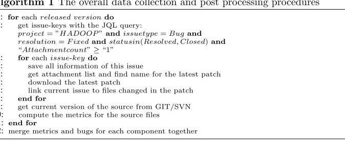
fil-tered out unresolved bugs and only considered fixed bugs with available patches. An issue is deemed to be a ‘fixed bug issue’ if its type attribute isBug, its reso-lution status isFixed, its status is eitherClosed orResolvedand the number of attachments is greater than one. We coded this rule as a ‘JQL’ query, using the JIRA command line tool to extract bug information automatically from the Hadoop JIRA repository. We examined the patches for each bug and located the source files that changed to fix it, considering only the latest patch version for multiply-patched bugs. For each Java class contained in a given revision, we computed the number of bugs found together with the Chidamber-Kemerer metrics [4] and the Lines of Code (LoC) metric using the toolckjm3. The overall data collection and post-processing procedures are described in Algorithm 1.
We analysed the first 8 versions of Hadoop Common (from 0.0.1 to 0.8.0) containing in total 16 minor releases. From these releases we extracted 626 bug fixes. We filtered out those affecting non java-components and the components contained in the package’s tests and examples. This left 509 bug fixes with which we experimented. For each version, we aggregated the data for all the correspond-ing revisions and considered a class to be faulty if its number of bugs is greater than 1. Considering all revisions together, 81% of the components are non-faulty
2
and 19% are faulty. To save space and support replication, all our data, statistics and results are available on-line4.
Algorithm 1 The overall data collection and post processing procedures
1: foreachreleased versiondo 2: get issue-keys with the JQL query:
project= ”HADOOP”andissuetype=Bugand resolution=F ixedandstatusin(Resolved, Closed)and
“Attachmentcount”≥“1”
3: foreachissue-keydo
4: save all information of this issue
5: get attachment list and find name for the latest patch
6: download the latest patch
7: link current issue to files changed in the patch
8: end for
9: get current version of the source from GIT/SVN
10: compute the metrics for the source files
11: end for
12: merge metrics and bugs for each component together
[image:4.612.143.480.151.289.2]3
Results
Figure 1 presents boxplots for G-mean and Recall values obtained over 30 runs for all models described in Section 2 and for Random Guessing (RG).
We observe that the best among the two models (MtorM Pt) performs in gen-eral better than RG. One-tailed Wilcoxon Sign Rank tests with Holm-Bonferroni corrections (overall α= 0.05) revealed that GA+SVM was significantly better than RG (with high effect size: ˆA12>0.81) in terms of G-mean on all the
con-sidered versions, except for t= 5 where there was no statistical difference. The best among the two models is significantly better than RG in terms of Recall on all the considered versions (with high effect size: ˆA12>0.80).
We now compare the performance of model Mt, against the corresponding model M Pt, to assess whether models trained on all data outperform those trained solely on the previous version.
Figure 1 reveals that the prediction ability of the modelsMtandM Ptvaries depending on the version. In particular, Mtprovided better G-mean thanM Pt on all the versionsvt+1except fort= 1, whileM P1 provided the best G-mean.
This is expected; early versions offer less information. However, Mt provided better Recall values than M Pt only in two cases (t = 2 and t = 6), similar in one case (t= 3), and worse in the remaining ones (t= 1,t= 4,t= 5).
To assess whether these differences are significant we used the Wilcoxon Signed Rank Test with Holm-Bonferroni corrections (overallα= 0.05). In partic-ular, we check two null hypotheses: HG0−mean: “There is no difference between the G-mean provided by Mt and its correspondingM Pt”; and HRecall0 :“There is no
difference between the Recall provided byMtand its correspondingM Pt”. The results revealed that we can reject HG0−meanfor all the versions (p-value<0.001), while we can reject HRecall
0 for all the models (p-value<0.005), except for t= 3
(p-value=0.145). We conclude that (a) there is always statistically significant difference between the G-mean values provided byMtandM Pt(and with high effect size: ˆA12>0.80) and this difference favours Mt, except fort= 1 where it
4
favoursMPt; (b) there is statistically significant difference between the Recall
values provided byMtandMPt(and with high effect size: ˆA12>0.70): in three
cases (t= 1,t = 4,t= 5) this difference favours MPt, in two cases (t = 2 and
t= 6) it favoursMt.
These findings from Hadoop indicate that engineers who want to find all faulty components may get better results using models trained solely on the previous version, discarding the extra ‘information’ present in the version history.
Since these results indicate that modelsMPtare potentially useful, we now move
on to investigate them in more detail.
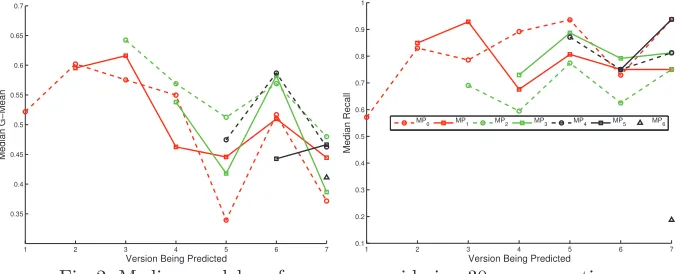
We investigate the performance of a model,MPt, built from versiont, at
pre-dicting faults in each and all of the subsequent versions. Figure 2 shows the me-dian performances. We observe that the G-mean does not always decrease with
time (e.g., MP3 and MP4), even though earlier models (e.g.,MP0 and MP1)
do tend to become less competitive with time. Once again, Recall is different. We see a lower variation in performance and also, perhaps more importantly, we observe models that remain competitive over many subsequent releases. For
instance, MP0 remains competitive throughout most of the first 8 versions of
Hadoop. We also observe that models trained on the most recent version are not
always the best fault predictors (e.g.,MP3outperformsMP5for fault prediction
in versionv6). This suggests that dynamic adaptive prediction systems [11, 10]
are required, so that we can automatically recognise the best-suited model for each version.
M0=MPO RG0 M1 MP1 RG1 M2 MP2 RG2 M3 MP3 RG3 M4 MP4 RG4 M5 MP5 RG5 M6 MP6 RG6
0.3
0.4
0.5
0.6
0.7
M0=MPO RG0 M1 MP1 RG1 M2 MP2 RG2 M3 MP3 RG3 M4 MP4 RG4 M5 MP5 RG5 M6 MP6 RG6
0.2
0.4
0.6
0.8
1.0 (a)
[image:5.612.140.481.393.518.2](b)
Fig. 1: G-mean (a) and Recall (b) obtained byMt,MPtand RG for predicting
faults in version vt+1, over 30 runs
1 2 3 4 5 6 7
0.35 0.4 0.45 0.5 0.55 0.6 0.65 0.7
Version Being Predicted
Median G−Mean
1 2 3 4 5 6 7
0.1 0.2 0.3 0.4 0.5 0.6 0.7 0.8 0.9 1
Version Being Predicted
Median Recall
MP
0 MP1 MP2 MP3 MP4 MP5 MP6
[image:5.612.138.478.560.697.2]4
Conclusions
Our analysis of Hadoop showed that using data from all versions is not always needed for prediction. We also found that prediction models trained on early software versions may preferable to those trained on the latest versions. This motivates the further study of dynamic adaptive fault prediction systems.
References
1. Afzal, W., Torkar, R.: On the application of genetic programming for software en-gineering predictive modeling: A systematic review. Expert Systems Applications 38(9), 11984–11997 (2011)
2. Arcuri, A., Briand, L.: A practical guide for using statistical tests to assess ran-domized algorithms in software engineering. In: ICSE. pp. 1–10 (2011)
3. Bouktif, S., Sahraoui, H., Antoniol, G.: Simulated annealing for improving software quality prediction. In: GECCO. vol. 2, pp. 1893–1900 (2006)
4. Chidamber, S.R., Kemerer, C.F.: A metrics suite for object oriented design. IEEE TSE 20(6), 476–493 (1994)
5. Di Martino, S., Ferrucci, F., Gravino, C., Sarro, F.: A genetic algorithm to configure support vector machines for predicting fault-prone components. In: PROFES 2011, LNCS, vol. 6759, pp. 247–261. Springer Berlin Heidelberg (2011)
6. Elish, K.O., Elish, M.O.: Predicting defect-prone software modules using support vector machines. JSS 81(5), 649–660 (2008)
7. Ferrucci, F., Harman, M., Sarro, F.: Search based software project management. In: Ruhe, G., Wohlin, C. (eds.) Software Project Management in a Changing World. Springer (2014), to appear
8. Gondra, I.: Applying machine learning to software fault-proneness prediction. JSS 81(2), 186–195 (2008)
9. Hall, T., Beecham, S., Bowes, D., Gray, D., Counsell, S.: A systematic literature review on fault prediction performance in software engineering. IEEE TSE 38(6), 1276–1304 (2012)
10. Harman, M.: How SBSE can support construction and analysis of predictive models (keynote). In: PROMISE (2010)
11. Harman, M., Burke, E., Clark, J.A., Yao, X.: Dynamic adaptive search based software engineering. In: ESEM. pp. 1–8 (2012)
12. Harman, M., McMinn, P., Souza, J., Yoo, S.: Search based software engineering: Techniques, taxonomy, tutorial. In: LNCS 7007, pp. 1–59 (2012)
13. He, H., Garcia, E.A.: Learning from imbalanced data. IEEE TKDE 21(9), 1263– 1284 (2009)
14. Krogmann, K., Kuperberg, M., Reussner, R.: Using genetic search for reverse en-gineering of parametric behaviour models for performance prediction. IEEE TSE 36(6), 865–877 (2010)
15. Minku, L., Yao, X.: Can cross-company data improve performance in software effort estimation? In: PROMISE. pp. 69–78 (2012)
16. Minku, L., Yao, X.: How to make best use of cross-company data in software effort estimation? In: ICSE. pp. 446–456 (2014)
17. Ostrand, T.J., Weyuker, E.J.: How to measure success of fault prediction models. In: SOQUA 2007. pp. 25–30. ACM (2007)
18. Rodriguez, D., Ruiz, R., Riquelme-Santos, J.C., Harrison, R.: Subgroup discovery for defect prediction. In: SSBSE. vol. 6956, pp. 269–270 (2011)