R E S E A R C H
Open Access
A generalized Newton method of
high-order convergence for solving the
large-scale linear complementarity problem
Yajun Xie
1,2and Changfeng Ma
1,2**Correspondence:
1School of Mathematics and
Computer Science, Fujian Normal University, Fuzhou, 350117, China
2Department of Mathematics and
Physics, Fujian Jiangxia University, Fuzhou, 350108, China
Abstract
In this paper, by extending the classical Newton method, we present the generalized Newton method (GNM) with high-order convergence for solving a class of large-scale linear complementarity problems, which is based on an additional parameter and a modulus-based nonlinear function. Theoretically, the performance of high-order convergence is analyzed in detail. Some numerical experiments further demonstrate the efficiency of the proposed new method.
MSC: 15A24; 65H10; 65F10; 65F30
Keywords: linear complementarity problem; generalized Newton method; high-order convergence; the modulus-based nonlinear function; additional parameter; numerical test
1 Introduction
We consider the linear complementarity problem, abbreviated asLCP(q,A), to find a vec-toru∈Rnsuch that
⎧ ⎪ ⎨ ⎪ ⎩
u≥,
w:=Au+q≥, wTu= ,
(.)
whereA∈Rn×nandq∈Rnare a given real matrix and a real vector, respectively. The linear complementarity problem frequently arises in various scientific and engi-neering applications, such as Nash equilibrium point of a bimatrix game, the contract problem, and the free boundary problem for journal bearings; see [–].
In [], Lemke proposed first a solution for linear complementarity problem. Along these ideas, Scarf has given the approximation of fixed-points of a continuous mapping []. The relationship between the linear complementarity problem and the fixed-points problem is well described by Eaveset al.[, ].
Many efficient methods were developed to solve linear complementarity problem. Es-pecially, when the system matrixAis large and sparse. For instance, we have the projected successive overrelaxation iteration [] and the general fixed-point iterations []. On the
matrix splitting iterations approaches, Baiet al.have derived some fruitful research re-sults [–], especially, in [], Bai proposed the modulus-based matrix splitting iteration scheme which is a powerful method for solving the linear complementarity problem. Ma-trix multisplitting iteration aspects, also, in many works were considered by Baiet al.to solve the linear complementarity problem in [–]. A variety of accelerated modulus-based matrix splitting iteration versions were also established; see [, ]. Furthermore, the modulus-based synchronous multisplitting iteration methods for large sparse linear complementarity problems are introduced in []. On the basis of [], Ljiljana et al. avoided the assumption of the parameter constraint and improved the convergence area []. Recently, in [], by the vector divisions and the secant method, Foutayeniet al. in-vestigated an efficient hybrid method for solving the linear complementarity problem.
As is well known the semismooth (or smooth) Newton method is very efficient for some nonsmooth (or smooth) equations, which arise from the complementarity problem, the nonlinear programming problem, the variational inequality problem, the discretization problem of partial differential equations, the maximal monotone operator problem,etc.; see [–] for a detailed discussion. These methods are competitive since they converge rapidly for any sufficiently right initial guess. In order to ensure that the global convergence of semismooth Newton methods, some merit functions, such as squared norm merit func-tions, are often exploited; see [] and the references therein. However, just as the state-ment in [], a globalization of the semismooth Newton method for nonsmooth equations is very hard because the corresponding merit function is nondifferentiable in most cases. In view of this, by introducing a smooth equation and some reasonable equivalent re-formulations, we investigate a generalized Newton iteration method with high-order con-vergence rate for solving a class of large-scale linear complementarity problem, which make full use of the superiority of the second-order convergence rate of the classical New-ton method. In this article, we suppose that the matrixAof the linear complementarity problem (.) is aP-matrix,i.e., the determinants of all principal submatrices are positive. Under this assumption, as is well known, the linear complementarity problem (.) has a unique solution for everyq.
For simplicity of the presentation, we use the following notations throughout the paper: LetNk={, , . . . ,k}denote the set of firstkpositive integers. Forx∈Rn,xstands for the Euclidean norm. Given two realn×mmatricesA= (aij) andB= (bij), we writeA≥B (orA>B) ifaij≥bij(oraij>bij) hold for alli∈Nnandj∈Nm.|A|andρ(A) denote the absolute value and spectral radius of the matrixA∈Rn×m, respectively. For a differential functionF(x),F(x) is referred to as the Jacobi matrix of the functionF(x). For an invertible matrixA,A–denotes the inverse matrix ofA. The matrixDiag{a,a, . . . ,a
n}denotes the diagonal matrix, whereai(i∈Nn) are the elements of the principal diagonal.
The outline of the paper is organized as follows. In Section , we first consider a gener-alized Newton method (GNM) with high-order convergence rate for solving a class of the linear complementarity problems (.). In Section , we analyze the performance and rate of convergence of the GNIM in detail. Some numerical experiments are given to illustrate that the GNM is efficient in Section . At last, we end the paper with some conclusions in Section .
2 The generalized Newton method
analysis of the convergence rate of the generalized Newton iteration method which will be presented in the following.
Lemma . The LCP(q,A) (.)is equivalent to the system of nonlinear equations
(I+A)x+ (I–A)|x|–q= , (.)
where A,q are given matrix and vector in(.),respectively.I is an identity matrix with appropriate dimension,x∈Rnis a vector to be determined.
Proof Letxbe the solution of equation (.). Then it yields
|x|+x=A|x|–x+q. (.)
Set
w:=|x|+x, u:=|x|–x. (.)
It is apparent from (.) and (.) that
w=Au+q, w≥,u≥, and wTu= ,
which means thatuis the solution ofLCP(q,A) (.).
On the other hand, we assumeuis the solution ofLCP(q,A) (.). It is obvious that
w≥, u≥, wTu= , wherew:=Au+q.
We also set
w:=|x|+x, u:=|x|–x,
it turns out that
x= (w–u)
satisfies equation (.).
Now, we introduce the smooth functionF:Rn+→Rnby
F(z) := (I–A)√x+εe+ (I+A)x–q, (.)
wherez= (ε,xT)T∈Rn+,εis a positive variable, e is a vector with all elements equal , i.e., e = (, , . . . , )T∈Rn,
√
x+εe:= x
+ε, x+ε, . . . , xn+ε T
We further define the nonlinear and differentiable function (z) := ε F(z)
∈Rn+. (.)
Lemma . LCP(q,A) (.)is equivalent to the nonlinear system
(z) = , (.)
where(z)is defined by(.),z= (ε,xT)T∈Rn+.
Proof The conclusion can easily be drawn by equation (.) and Lemma ..
Lemma . The Jacobi matrix of equation(.)is
(z) =
(I–A)gε (I–A)Dx+A+I
∈R(n+)×(n+), (.)
where g(ε) = (g,g, . . . ,gn)T ∈ Rn, gi = √ε x
i+ε
, Dx =Diag(d,d, . . . ,dn) ∈Rn×n, di = xi
√
xi+ε,i∈Nn,and∈R
×nis a zero vector.
Proof It follows from the derivatives for the variablezon both sides of equation (.) that
(z) =
Fε Fx
. (.)
According to equations (.) and (.), we immediately have
Fε= (I–A)
ε
x
+ε , ε
x +ε
, . . . , ε x
n+ε T
∈Rn (.)
and
Fx= (I–A)Diag
x
x +ε
, x x
+ε
, . . . , xn x
n+ε
+A+I∈Rn×n. (.)
This completes the proof.
Now, we show the generalized Newton iteration method for the nonlinear smooth sys-tem (.). A detailed description follows.
Algorithm .(The generalized Newton method)
Step Input the initial guessz= (ε, (x)T)T, give the matrixAand vectorqand any small positive numbersσ,σ∈(, ), preset a positive integerm≥. Setk:= .
Step Compute(zk), the Jacobi matrix(zk), and its inverse matrixA
k:= ((zk))–.
Step Setzk,=zk,j:= .
Step Evaluate(zk,j), update the vector sequence
zk,j+=zk,j–Akb,
Step Setj:=j+ ,zk,j=zk,j+,(zk,j) =(zk,j+),y:=A
kb. Ifj=m, return to Step , otherwise go to Step .
Step Ify<σor(zk,m)<σ, letzk,m=z∗, otherwisek:=k+ , return to Step .
The generalized Newton iteration method (GNIM) also can be written with the follow-ing iterative scheme:
⎧ ⎪ ⎨ ⎪ ⎩
zk,=zk,
zk,j=zk,j–– ((zk))–(zk,j–), j= , , . . . ,m, xk+=xk,m, k= , , , . . . .
(.)
Remark . From Lemma ., we know that the iterative solutionz∗generated by Algo-rithm . is also the solutionu∗ofLCP(q,A) (.).
Remark . The update of parameterεk can be chosen withεk=εkm–. Since the posi-tive integermis selected at least greater than or equal to in Algorithm ., the positive sequence{εk}∞ declines monotonically and tends to zero.
Remark . Once we setm= , then the GNIM reduces to the classical Newton iterative method.
3 The analysis of convergence
Definition . ([]) LetF:D⊂Rn→Rn, x∗∈Dis the solution of system F(x) = . There is a regionS⊂Dfor the pointx∗, for any initial approximationx∈S, if the iteration sequence{xk,k= , , . . .}is always well defined and converges tox∗, we call it the attractive point of the iteration sequence.
The classical Newton iteration features a convergence rate of at least order two. We have the following results; for more details see [] and the references therein.
Lemma .([]) Let F:D⊂Rn→Rnbe Frechet differentiable on the open interval of´ S∈D,and F(x∗)be nonsingular,where x∗ is the solution of system F(x) = .Then the mapping G(x) =x–F(x)–F(x)is well defined on S for the closed sphere S=S(x¯ ∗,δ)⊂S. Moreover,if the inequality
F(x) –Fx∗≤βx–x∗ (.)
holds,whereβis a constant,x∈S,then the classical Newton iteration method has at least a convergence rate of order two.
Lemma .([]) Let F:D⊂Rn→Rnbe Fréchet differentiable on the fixed-point x∗∈ int(D),and the spectral radius of F(x∗)
ρFx∗=σ≤. (.)
Lemma .[] Let F:D⊂Rn→Rmbe continuous and differentiable on the convex set D⊂D,and satisfy
F(u) –F(v)≤βu–vp, u,v∈D. (.)
Then we have
F(y) –F(x) –F(x)(y–x)≤ β
+py–x
+p, x,y∈D
, (.)
where the constantsβ≥,p≥.
We are now in a position to derive the main convergence result of the generalized New-ton iteration method.
Theorem . Let:D⊂Rn+→Rn+ be Fr´echet differentiable on the circle region of S(z∗,δ)∈D,and(z∗)be nonsingular,where z∗is the solution of(z) = .Assume that for arbitrary z∈S,there is a constantβ> such that
(z) –z∗≤βz–z∗ (.)
holds.Then z∗ is the attractive point of the iterative sequence{zk}∞
generated by Algo-rithm.,and
zk+–z∗≤Lzk–z∗m+, (.)
where Lis a constant independent of iteration number k.
Proof To begin with, we consider the iterative equation (.) with the casem= ,i.e.,
zk+=zk–zk–zk–zk–zk–zk, k= , , . . . . (.)
By applying Lemma .,P(z) :=z– ((z))–(z) is well defined onS:=S(z¯ ∗,δ)⊂Sand P(z) –z∗≤ξzk–z∗, z∈S, (.)
whereξ is a positive constant. Hence, the mappingM(z) =P(z) – ((z))–(P(z)) is well defined on the closed sphereS=S(z¯ ∗,δ)⊂S, whereδ≤δξ and
Mz∗=I–z∗–Pz∗= .
So,ρ(M(z∗)) = < . It follows from Lemma . thatz∗is the attractive point of equation (.).
On the other hand, note the nonsingularity of(z∗), hence((z))– ≤ζ forz∈S. Then it follows from Lemma . and the assumptions that
M(z) –z∗≤(z)–(z)P(z) –z∗–P(z)
+z∗–(z)P(z) –z∗
≤ζ
βP(z) –z
∗
+βz–z∗P(z) –z∗
≤βζ
ξ
z–z∗+ξz–z∗
≤βζ ξ
ξ δ+
z–z∗. (.)
LetL:=βζ ξ[ξ δ+ ], evidently, it is a constant independent of the iteration numberk. When we choosezk+=M(zk) for the left of the inequality (.), it yields
zk+–z∗≤Lzk–z∗
, (.)
which implies (.) holds form= .
Now, we state that the iterative scheme (.) has at least a convergence rate of order m+ . The result will be shown by mathematical induction.
Noting that (.), one has the argument
zk,–z∗≤Lzk–z∗=Ozk–z∗. (.)
Next, we assume that
zk,m––z∗≤Lzk–z∗ m
=Ozk–z∗m (.)
holds. Now, we will verify the statement
zk,m–z∗≤Lzk–z∗m+=Ozk–z∗m+, (.)
whereL,Lare constants independent of the iteration numberk.
As a matter of fact, observing (.), also by Lemma . and (.), one obtains
zk,m–z∗≤zk–zk,m––z∗–z∗zk,m––z∗
+z∗–zkzk,m––z∗
≤ζ
βz
k,m––z∗+βzk–z∗zk,m––z∗
≤ζβ
L
zk–z∗ m–
+L
zk–z∗m+
≤ζβ
L
δm–+L
zk–z∗m+
=Lzk–z∗ m+
=Ozk–z∗m+, (.)
4 Numerical experiments
In this section, we report some numerical results to illustrate the effectiveness of the GNIM for solving the linear complementarity problem. We compare the GNIM with the Fischer-based semismooth Newton method which we call FBSN (see [, ]), and the cosh-based smoothing Newton method which we call CBSN (see []) by the iteration step (denoted as ‘IT’), the elapsed CPU time in seconds (denoted as ‘CPU’), and the resid-ual error (denoted as ‘RES’). In actresid-ual computations, all runs are terminated if the current iterations satisfy
RES:=zk< –,
or if the number of iterations exceeds the prescribed number of iteration steps kmax. The numerical experiments have been carried out by MATLAB Rb (.), Intel(R) Core(TM) i-QM, CPU .GHZ, RAM .GB PC Environment, and Windows op-erating system.
In fact, our approach can be considered as the version of speeding up on the basis of the smoothing Newton method. Thereby, high precision is the advantage of the GNIM. Once we setm= , the GNIM will reduce to the classical Newton method. But we know that the largermmay lead to the consumption of more CPU time since there is an increased number of inner iterations. We usually choosem= in concrete tests, which also can ensure the rapid convergence rate. To confirm this judgment, we can observe the following examples.
Example .([]) We consider the linear complementarity problem (.) with
A=tridiag(–, , –), q= (–, . . . , –)T.
Example . We consider the linear complementarity problem (.) withA= (aij),i,j∈
Nn, whereaij= iδij
n,δis the Kronecker delta (δii= ,δij= , wheni=j), andq= (qi),i∈Nn such thatqi= –.
In these examples, we choosem= for the GNIM, andρ= .,β= .,p= . for the FBSN (for more details, see []). Especially, the RES will be regarded as ifRES< – in the numerical results. The initial guess will be selected withz
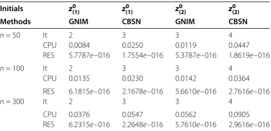
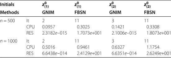
()orz()by [ε,qT]Tor the zero vector, respectively. First, we compare the performance of the numerical results of the GNIM with the CBSN by arranging differentn. From Tables and , we find the GNIM and the CBSN are all effective methods whose solution pairs (u∗,w∗) are also displayed in the last column of tables. However, from the aspects of the iteration number or CPU, the CBSN does not stand comparison with our method. In Table , we provide the numerical results for the GNIM and the CBSN with larger dimensions. Furthermore, the merit of the GNIM is reflected clearly and incisively.
It is observed from Table that the GNIM is much more competitive than the FBSN for the large-scale linear complementarity problem. The numerical results of Example . is shown by Tables -. Especially, from Table , we find that the FBSN is unable to obtain the convergence result in less iteration steps, such as within , for Example ..
Table 1 The GNIM numerical results for Example 4.1 with initialz0(1)
The performance of numerical results
The solution pairs(u∗, w∗)
n= 3 It 3 u∗= (0.3571, 0.4286, 0.3571) CPU 0.0068
RES 0 w∗= (0, 0, 0)
n= 5 It 3 u∗= (0.3654, 0.4615, 0.4808, 0.4615, 0.3654) CPU 0.0073
RES 0 w∗= 1.0e–015∗(0.4441, 0, 0, 0, 0)
n= 8 It 3 u∗= (0.3660, 0.4641, 0.4902, 0.4967, 0.4967, 0.4902, 0.4641, 0.3660) CPU 0.0074
RES 0 w∗= (0, 0, 0, 0, 0, 0, 0, 0)
n= 10 It 3 u∗= (0.3660, 0.4641, 0.4904, 0.4974, 0.4991, 0.4991, 0.4974, 0.4904, 0.4641, 0.3660) CPU 0.0075
[image:9.595.151.442.335.529.2]RES 0 w∗= 1.0e–015∗(–0.1110, 0.4441, –0.4441, 0, 0, 0, 0.2220, 0, 0, 0)
Table 2 The CBSN numerical results for Example 4.1 with initialz0(1)
The performance of numerical results
The solution pairs(u∗, w∗)
n= 3 It 4 u∗= (0.3571, 0.4286, 0.3571) CPU 0.0104
RES 0 w∗= 1.0e–011∗(0.8880, –0.5869, 0.8880)
n= 5 It 4 u∗= (0.3654, 0.4615, 0.4808, 0.4615, 0.3654) CPU 0.0106
RES 6.1063e–016 w∗= 1.0e–015∗(0, 0, 0, 0, –0.1110)
n= 8 It 4 u∗= (0.3660, 0.4641, 0.4902, 0.4967, 0.4967, 0.4902, 0.4641, 0.3660)
CPU 0.0113
RES 6.2042e–016 w∗= 1.0e–011∗(0.4839, –0.1609, –0.0001, 0, 0, – 0.0001, –0.1608, 0.4839)
n= 10 It 3 u∗= (0.3660, 0.4641, 0.4904, 0.4974, 0.4991, 0.4991, 0.4974, 0.4904, 0.4641, 0.3660) CPU 0.0115
RES 6.2232e–016 w∗= 1.0e–011∗(0.4835, –0.1607, –0.0001, 0, 0, 0, 0, –0.0001, –0.1607, 0.4835)
Table 3 Numerical results for Example 4.1
Initials z0
(1) z(1)0 z(2)0 z(2)0
Methods GNIM CBSN GNIM CBSN
n= 50 It 2 3 3 4
CPU 0.0084 0.0250 0.0119 0.0447
RES 5.7787e–016 1.7554e–016 5.3787e–016 1.8619e–016
n= 100 It 2 3 3 4
CPU 0.0135 0.0230 0.0142 0.0364
RES 6.1815e–016 2.1678e–016 5.6610e–016 2.7616e–016
n= 300 It 2 3 3 4
CPU 0.0376 0.0547 0.0562 0.0905
[image:9.595.164.432.572.702.2]Table 4 Numerical results for Example 4.1
Initials z0(1) z0(1) z(2)0 z0(2)
Methods GNIM FBSN GNIM FBSN
n= 500 It 2 11 3 11
CPU 0.0886 0.3229 0.1366 0.3831
RES 6.1815e–016 6.6613e–016 5.6610e–016 1.1047e–015
n= 1000 It 2 11 3 11
CPU 0.5114 1.0758 0.7728 1.3069
RES 6.2113e–016 6.6723e–016 5.6720e–016 1.3027e–015
n= 3000 It 2 11 3 11
CPU 9.1418 26.6155 11.1484 11.5429
RES 6.2812e–016 6.6921e–016 5.5610e–016 1.2123e–015
n= 5000 It 2 11 3 11
CPU 42.9507 71.3675 66.0831 79.3341
[image:10.595.151.444.314.491.2]RES 6.4615e–016 6.6990e–016 5.7810e–016 1.3056e–015
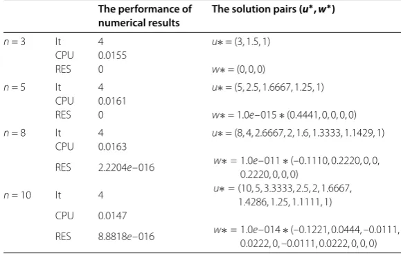
Table 5 The GNIM numerical results for Example 4.2 with initialz0(1)
The performance of numerical results
The solution pairs(u∗, w∗)
n= 3 It 2 u∗= (3, 1.5, 1)
CPU 0.0067
RES 0 w∗= (0, 0, 0)
n= 5 It 2 u∗= (5, 2.5, 1.6667, 1.25, 1) CPU 0.0070
RES 0 w∗= 1.0e–015∗(0.2220, 0, 0, 0, 0)
n= 8 It 2 u∗= (8, 4, 2.6667, 2, 1.6, 1.3333, 1.1429, 1) CPU 0.0072
RES 0 w∗= (0, 0, 0, 0, 0, 0, 0, 0)
n= 10 It 2 u∗= (10, 5, 3.3333, 2.5, 2, 1.6667, 1.4286, 1.25, 1.1111, 1)
CPU 0.0075
RES 0 w∗= 1.0e–015∗(0, 0.2220, –0.1110, 0, 0, 0, 0.2220, 0, 0, 0)
Table 6 The CBSN numerical results for Example 4.2 with initialz0(1)
The performance of numerical results
The solution pairs(u∗, w∗)
n= 3 It 4 u∗= (3, 1.5, 1)
CPU 0.0155
RES 0 w∗= (0, 0, 0)
n= 5 It 4 u∗= (5, 2.5, 1.6667, 1.25, 1) CPU 0.0161
RES 0 w∗= 1.0e–015∗(0.4441, 0, 0, 0, 0)
n= 8 It 4 u∗= (8, 4, 2.6667, 2, 1.6, 1.3333, 1.1429, 1) CPU 0.0163
RES 2.2204e–016 w∗= 1.0e–011∗(–0.1110, 0.2220, 0, 0, 0.2220, 0, 0, 0)
n= 10 It 4 u∗= (10, 5, 3.3333, 2.5, 2, 1.6667, 1.4286, 1.25, 1.1111, 1) CPU 0.0147
[image:10.595.151.441.549.732.2]Table 7 Numerical results for Example 4.2
Initials z0(1) z(1)0 z0(2) z0(2)
Methods GNIM FBSN GNIM FBSN
n= 500 It 2 11 3 11
CPU 0.0957 0.3025 0.1421 0.3308
RES 2.3182e–015 1.7073e+001 2.1006e–015 1.8073e+001
n= 1000 It 2 11 3 11
CPU 0.5016 0.9461 0.6327 1.1754
RES 6.6438e–014 2.4129e+001 6.6351e–014 2.6249e+001
5 Conclusion
In this paper, we establish the generalized Newton method (GNM) for solving the large-scale linear complementarity problem. The GNM features the high-order convergence rate, at least convergence orderm+ , which has been verified from theoretical analysis section in detail. The new strategy will increase the efficiency remarkably. In fact, it can be regarded as an accelerated process for the classical Newton approach. Experimental tests provide the comparison of the numerical performance for some existing efficient methods, which testify to the viability of the proposed approach.
Competing interests
The authors declare that there is no conflict of interests regarding the publication of this article.
Authors’ contributions
All authors contributed equally and significantly in writing this article. All authors read and approved the final manuscript.
Acknowledgements
The Project Supported by National Natural Science Foundation of China (Grant Nos. 11071041, 11201074), Fujian Natural Science Foundation (Grant Nos. 2015J01578, 2013J01006) and The Outstanding Young Training Plan of Fujian Province universities (Grant No. 15kxtz13, 2015).
Received: 8 October 2015 Accepted: 8 December 2015
References
1. Cottle, RW, Pang, J-S, Stone, RE: The Linear Complementarity Problem. Academic Press, San Diego (1992) 2. Murty, KG: Linear Complementarity, Linear and Nonlinear Programming. Heldermann, Berlin (1988) 3. Lemke, CE: Bimatrix equilibrium points and mathematical programming. Manag. Sci.11, 681-689 (1965) 4. Scarf, H: The approximation of fixed points of a continuous mapping. SIAM J. Appl. Math.15, 1328-1342 (1967) 5. Eaves, BC, Scarf, H: The solution of systems of piecewise linear equations. Math. Oper. Res.1, 1-27 (1976) 6. Eaves, BC, Lemke, CE: Equivalence of LCP and PLS. Math. Oper. Res.6, 475-484 (1981)
7. Cryer, C: The solution of a quadratic programming using systematic overrelaxation. SIAM J. Control Optim.9, 385-392 (1971)
8. Tseng, P: On linear convergence of iterative method for the variational inequality problem. J. Comput. Appl. Math.60, 237-252 (1995)
9. Bai, Z-Z: Modulus-based matrix splitting iteration methods for linear complementarity problems. Numer. Linear Algebra Appl.17, 917-933 (2010)
10. Bai, Z-Z, Evans, DJ: Matrix multisplitting methods with applications to linear complementarity problems: parallel synchronous and chaotic methods. In: Calculateurs Parallèles Réseaux et Systèmes Répartis, vol. 13, pp. 125-141 (2001)
11. Bai, Z-Z, Evans, DJ: Matrix multisplitting methods with applications to linear complementarity problems: parallel asynchronous methods. Int. J. Comput. Math.79, 205-232 (2002)
12. Bai, Z-Z, Zhang, L-L: Modulus-based synchronous multisplitting iteration methods for linear complementarity problems. Numer. Linear Algebra Appl.20, 425-439 (2013)
13. Bai, Z-Z: On the convergence of the multisplitting methods for the linear complementarity problem. SIAM J. Matrix Anal. Appl.21, 67-78 (1999)
14. Bai, Z-Z, Evans, DJ: Matrix multisplitting relaxtion methods for linear complementarity problem. Int. J. Comput. Math. 63, 309-326 (1997)
15. Bai, Z-Z: Experimental study of the asynchronous multisplitting relaxtation methods for linear complementarity problems. J. Comput. Math.20, 561-574 (2002)
16. Bai, Z-Z, Huang, Y-G: A class of asynchronous iterations for the linear complementarity problem. J. Comput. Math.21, 773-790 (2003)
18. Zhang, L-L: Two-step modulus based matrix splitting iteration for linear complementarity problems. Numer. Algorithms57, 83-99 (2011)
19. Zheng, N, Yin, J-F: Accelerated modulus-based matrix splitting iteration methods for linear complementarity problem. Numer. Algorithms64, 245-262 (2013)
20. Bai, Z-Z, Zhang, L-L: Modulus-based synchronous multisplitting iteration methods for large sparse linear complementarity problem. Numer. Linear Algebra Appl.20, 425-439 (2013)
21. Ljiljana, C, Vladimir, K: A note on the convergence of the MSMAOR method for linear complementarity problems. Numer. Linear Algebra Appl.21, 534-539 (2014)
22. Foutayeni, YEL, Khaladi, M: Using vector divisions in solving the linear complementarity problem. J. Comput. Appl. Math.236, 1919-1925 (2012)
23. Qi, L, Sun, J: A nonsmooth version of Newton’s method. Math. Program.58, 353-368 (1993)
24. Jiang, H-Y, Qi, L: A new nonsmooth equations approach to nonlinear complementarity problems. SIAM J. Control Optim.35, 178-193 (1997)
25. Chen, X, Nashed, Z, Qi, L: Smoothing methods and semismooth methods for nondifferentiable operator equations. SIAM J. Numer. Anal.38, 1200-1216 (2000)
26. Pang, J-S: Newton’s method forB-differentiable equations. Math. Oper. Res.15, 311-341 (1990)
27. Sun, Z, Zeng, J-P: A monotone semismooth Newton type method for a class of complementarity problems. J. Comput. Appl. Math.235, 1261-1274 (2011)
28. Huang, X-D, Zeng, Z-G, Ma, Y-N: The Theory and Methods for Nonlinear Numerical Analysis, pp. 57-59. Wuhan University Press, Wuhan (2004)
29. Luca, D, Fancchinei, F, Kanzow, C: A semismooth equation approach to the solution of nonlinear complementarity problems. Math. Program.75, 407-439 (1996)
30. Fischer, A: A special Newton-type optimization method. Optimization24, 269-284 (1992)