Multigranulation Decision theoretic Rough Set Based on Incomplete Interval valued Information Systems

(1)

2018 2nd International Conference on Applied Mathematics, Modeling and Simulation (AMMS 2018) ISBN: 978-1-60595-580-3

Multigranulation Decision-theoretic Rough Set Based on Incomplete

Interval-valued Information Systems

Rui-kang XING

1,*

, Cheng-hai LI

1

, Xin ZHANG

1

and Fang-zheng ZHAO

1

1_{Academy of Anti-missile and Air Defense, Air Force Engineering University,}

Xi’an 710051, PR China

*Corresponding author

Keywords: Decision-theoretic rough set, Variable precision, Multi-cost.

Abstract. Most of the previous results about decision-theoretic rough set do not take a variety of decision maker’s attitude into consideration, which is vulnerable environmental impact in reality. To solve such problems, a strategy is firstly introduced into multigranulation decision-theoretic rough set by the definition of decision function. Firstly, the equivalence classes are replaced with maximal consistent classes to establish the decision-theoretic rough set in an incomplete interval-valued information system. Then, based on the definition of decision function, the Sigmoid-multigranulation decision-theoretic rough set model and generalized multigranulation decision-theoretic rough set model are proposed and some properties of two models are studied in an incomplete interval-valued information system. Finally, the relation is illustrated between generalized multigranulation decision-theoretic rough set model and other related rough set models. This study suggests potential application areas and new research trends concerning decision-theoretic rough set.

Introduction

Pawlak rough set theory[1] is a powerful mathematical tool for uncertainty management, especially in describing the uncertainty of the data. Rough set theory has been widely used in many fields such as data mining[2], machine learning[3], pattern recognition[4] and deep learning[5]. Nowadays, the various extensions of the rough set model have been proposed with different requirements, such as multigranulation rough set[6,7], decision-theoretic rough set[8,9], probabilistic rough set[10], variable precision rough set[11], fuzzy rough set[12] , intuitional fuzzy rough set[13] and rough set in incomplete information system[14].

In the view of granulation, the Pawlak rough set model describe the target concept under a single granulation. In order to describe target concept under multiple relation just like human beings, Qian et al.[6] proposed multigranulation rough set theory. The multigranulation rough set theory have been widely studied by researchers. The literature[24] extended multigranulation rough set model to an incomplete rough set model based on a tolerance relation. In reality, many practical decision making may relate to two or more different universes, Sun, B. et al.[15] proposed the multigranulation rough set based on two universes. In order to apply multigranulation decision-theoretic rough set to incomplete information system, Yang et al.[16] proposed three multigranulation decision-theoretic rough set models. The article[17] presented the multigranulation decision-theoretic rough set model in ordered information system. In terms of inclusion measure of fuzzy rough sets in the viewpoint of fuzzy multigranulation, Lin, G. et al.[18] proposed the fuzzy multigranulation decision-theoretic rough set model.

(2)

Multigranulation Decision-theoretic Rough Set

In incomplete interval-valued information systemIIIS U AT, , C C1, 2, ,Cm are attribute subsets of

AT, the set of actions is given by Aa a aP, B, N, where aP, aB and aN represent the three actions

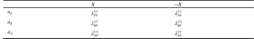
[image:2.595.79.511.177.244.2]

in classifying an object x. Under the ith granular’ describing, the loss functions are given in Table 1.

Table 1. The loss function under the ith granular structure.

X X

P

a  i

PP

  i

PN



B

a  i

BP

  i

BN



N

a  i

NP

  i

NN



Considering the reasonable kind of losses with  i  i  i PP BP NP

   ,  i  i  i NN BN PN

   .

Under the ith granular structure the expected loss



|  



i k C

R a M x associated with taking the action

 , , 

k

a kP B N for an object x can be expressed as:

 

     _{ }    _{ }

 

     _{ }    _{ }

 

     _{ }    _{ }

| | |

i i i

i i

P C PP C PN C

i i

B C BP C BN C

i i

N C NP C NN C

R a M x P X M x P X M x

  

 

  

，where      

| |

|

| |

i i

i

C C

C

M x X

P X M x

M x

 



 .

Yang[23] proposed optimistic multigranulation decision-theoretic rough set and pessimistic multigranulation decision-theoretic rough set based on the decision procedure of optimistic and pessimistic decision makers, respectively. The optimistic model’s lower and upper approximations are defined as follows:

    

 

    

, 1

1

1 1

|

1 | |

i

i i

m

C

m OI i

i m m

i

C C

i i

P X M x

C X x U

P X M x P X M x

 

  

 

 _ 

 

   

     

 



，

    

 

    

, 1

1

1 1

|

1 | |

i

i i

m

C

m OI i

i m m

i

C C

i i

P X M x

C X x U

P X M x P X M x

 

  

 

 _ 

 

   

     

 



And the pessimistic model’s lower and upper approximations are defined as follows:

    

 

    

, 1

1

1 1

|

1 | |

i

i i

m C

m OI i

i m m

i

C C

i i

P X M x

C X x U

P X M x P X M x

 

  

 

 _ 

 

   

     

 



    

 

    

, 1

1

1 1

|

1 | |

i

i i

m

C

m OI i

i m m

i

C C

i i

P X M x

C X x U

P X M x P X M x

 

  

 

 _ 

 

   

     

 



Sigmoid-multigranulation Decision-theoretic Rough Set

The optimistic model and the pessimistic model proposed in paper [27] are extreme. The optimistic and pessimistic decision makers are two special types of decision makers, there still exists other type of decision makers in reality. In this paper, we use the Sigmoid function to establish the decision function which represents the type of decision makers and set up the Sigmoid-multigranulation decision-theoretic rough set model. By the Sigmoid function, the decision function is defined as follow:

 1 

1 1 1

1 ; , ,

1

n n n

n i i i

i i i

x x x x x

e

  _

  

 

   _    

 

where  _{is the parameter to adjust the different decision makers’ attitude to the loss.}

When  , the decision maker is the optimistic one, the decision function is  ; ,1 ,  ₁

n n _i i

x x x

 

   ;

when  , the decision maker is the pessimistic one, the decision function is  ; ,1 ,  ₁

n n _i i

x x x

 

(3)

when 0, decision maker is moderate, the decision function is  1  1 1 1 ; , , 2 n n

n i i

i i

x x x x

 

 

 

 _   _

 .

Therefore, the expected loss associated with taking the action a_ P B N, ,  for an object x can

be expressed as:



_{ }    





 





 



 





 



_{ }









 



_{ }



 



_{ }



1 1 1 1 1 1 | , , ; | , , | ; | , , | ; | , , | m m m m

C C C C

m m

P C P C N C N C

R a M x M x R a M x R a M x

P X M x P X M x P X M x P X M x

                             

For _ i

, there are two case. One is that   i

 is irrelevant to i. Another is that   i

 is relevant to i.

In this paper, we assume that _ i

 is irrelevant to i. That is to say

 1    1    1    1    1    1  

, , , , ,

m m m m m m

PP PP PP BP BP BP NP NP NP PN PN PN BN BN BN NN NN NN

                       

We have



|



₁ , ,  





;



| ₁ 



, ,



|  





;



| ₁ 



, ,



|  



m m m

C C P C C N C C

R a_ M x M x   _ P X M x P X M x   _ P X M x PX M x

By Bayesian minimum-risk decision procedure, we have decision rules as follows: (P1) If R a



P|



MC1 x , ,MCm x



R a



B|



MC1 x , ,MCm x



  _   _and



   





   



1 1

| , , | , ,

m m

P C C N C C

R a M x M x R a M x M x ,

then xpos_

 

X ;

(B1) If R a



B|



MC1 x, ,MCm x



R a



P|



MC1 x, ,MCm x



  _  

and R a



B|



MC1 x , ,MCm x



R a



N|



MC1 x , ,MCm x



  _  

, then xbn X ;

(N1) If R a



N|



MC1 x, ,MCm x



R a



P|



MC1 x, ,MCm x



  _   _and



_{ } _{ }





_{ } _{ }



1 1

| , , | , ,

m m

N C C B C C

R a M x M x R a M x M x ,

then xneg X ;

Considering the b d b d  a b c d, , , 0

ac abcd   and PPBPNP, NNBNPN,the decision rules

(P1)~(N1) can be expressed concisely as:

(P1)If         

 

          

1 1 1

1 1 1 1

1

| | |

1

2

1 | | | |

1

i i i

i i i i

m m m

C C C

i i i

m m m m

C C C C

i i i i

P X M x P X M x P X M x e

P X M x P X M x P X M x P X M x e                        _ _   _         _ _   _ and                       

1 1 1

1 1 1 1

1

| | |

1

2

1 | | | |

1

i i i

i i i i

m m m

C C C

i i i

m m m m

C C C C

i i i i

P X M x P X M x P X M x

e

P X M x P X M x P X M x P X M x

e                        _ _   _         _ _   _

, then xpos_ X ;

(B1)If         

 

          

1 1 1

1 1 1 1

1

| | |

1

2

1 | | | |

1

i i i

i i i i

m m m

C C C

i i i

m m m m

C C C C

i i i i

e

e                        _ _   _         _ _   _ and                       

1 1 1

1 1 1 1

1

| | |

1

2

1 | | | |

1

i i i

i i i i

m m m

C C C

i i i

m m m m

C C C C

i i i i

P X M x P X M x P X M x e

P X M x P X M x P X M x P X M x e                        _ _   _         _ _   _

, thenxbn X ;

(N1)If         

 

          

1 1 1

1 1 1 1

1

| | |

1

2

1 | | | |

1

i i i

i i i i

m m m

C C C

i i i

m m m m

C C C C

i i i i

e

e                        _   _    _        _   _    and     _  _ _  _             

1 1 1

1 1 1 1

1

| | |

1

2

1 | | | |

1

i i i

i i i i

m m m

C C C

i i i

m m m m

C C C C

i i i i

e

e                        _ _   _         _   _   

, then xneg X ;

where P N B N B P P P P N B N

           

B N N N

N P B P B N N N

           

P N N N

N P P P P N N N

           

If PNBNNPBP  BNNNBPPP, then 0      1

Therefore, the Sigmoid-multigranulation positive, negative and boundary regions of Xcan be defined as follows:

          

 

          

1 1 1

1 1 1 1

1

| | |

1

2

1 | | | |

1

i i i

i i i i

m m m

C C C

i i i

m m m m

C C C C

i i i i

P X M x P X M x P X M x

e

pos X x U

P X M x P X M x P X M x P X M x

e                       _ _ _ _{ }              _ _        _   _                                

1 1 1

1 1 1 1

1

| | |

1

2

1 | | | |

1

i i i

i i i i

m m m

C C C

i i i

m m m m

C C C C

i i i i

e

neg X x U

(4)

            

          

1 1 1

1 1 1 1

1

| | |

1

2

1 | | | |

1

i i i

i i i i

m m m

C C C

i i i

m m m m

C C C C

i i i i

e

bn X x U

e

  

 



   



     



   

 _ _ _ _{ }  

 

 

    

    

 

 _{ } _{ } _ __ _{ } _ 

    

 

Definition 1. Let IIIS U AT, be an incomplete interval-valued information system,

1, 2, , m

C C C

are attribute subsets of AT, 0    1.  X U, the Sigmoid-multigranulation lower and upper approximation of X can be defined as follows: respectively:

          

 

          

1 1 1

, 1

1 1 1 1

1

| | |

1

2

1 | | | |

1

i i i

i i i i

m m m

C C C

i i i

m

i m m m m

i

C C C C

i i i i

e

C X x U

e

  

  

   







  





   

 _ _ _ _{ }  

 

 

    

  _ _ 

          

    

 



          

 

          

1 1 1

, 1

1 1 1 1

1

| | |

1

2

1 | | | |

1

i i i

i i i i

m m m

C C C

i i i

m

i m m m m

i

C C C C

i i i i

e

C X x U

e

  

  

   







  





   

 _ _ _ _{ }  

 

 

    

  _ _ 

          

    

 



The set pair ,   ,  

1 , 1

m m

i i

i C X i C X

   

 

 

 





 is the Sigmoid-multigranulation decision-theoretic rough

set.

When   , the decision maker is the optimistic one, the Sigmoid-multigranulation decision-theoretic rough set model is the optimistic multigranulation decision-theoretic rough set model; when  , the decision maker is the pessimistic one, the Sigmoid-multigranulation decision-theoretic rough set model is the pessimistic one; when 0, decision maker is moderate,

the lower and upper approximations are given by:

       

  _  _ _  _

,

1 1 1

,

1 1 1

1

| |

2

1

| |

2

i i

m m

m

i C C

i i i

m m

m

i C C

i i i

C X x U P X M x P X M x

   

   





  

   

  _   _ 

 

   

  _   _ 

 



Proposition 1. Let IIIS U AT, be an incomplete interval-valued information system,

1, 2, , m

C C C _{are attribute subsets of} AT, 0    1. We have:

(1) ,   ,  

1 1

m m

i i

i C X i C X

   

  



(2) ,   ,  

1 1

m m

i i

i C i C

   

      



,   ,  

1 1

m m

i i

i C U i C U U

   

   



(3) ,   ,1   

1 1 0.5

m m

i i

i C X i C X

    _

     



,   , 1  

1 1 0.5

m m

i i

i C X i C X

    _

     



(4) If 0 1 21 and 0121 then    

2 1

, ,

1 1

m m

i i

i C X i C X

   

  



and

   

2 1

, ,

1 1

m m

i i

i C X i C X

   

  



Generalized Multigranulation Decision-theoretic Rough Set

Different kind of decision makers have different approaches to deal with risk. Therefore, the function curves are different between decision makers. In reality, there may exist various kinds of decision makers, the Sigmoid-multigranulation decision-theoretic rough set model just account for a special type. However, the same kind decision makers may have different strategy to deal with risk with the effect of time, place and so on. At present, some multigranulation decision-theoretic rough set models have been established with the different requirement. The research for generalized multigranulation decision-theoretic rough set is necessary.

Definition 2. _Let    , _{is a parameter to adjust the different decision makers’ attitude to}

the risk. The t1, ,tl represent the elements which affect decision makers, such as time, place and so

on. We define the function f, ,t1 , ; ,t xl 1 ,xm as decision function, if the function satisfy:

(1) f, ,t1 , ; ,t xl 1 ,xmmin , maxxi xi; (2) f, ,t1 , ;0,tl ,00;

(3) _xlim_f, ,t1 , ; ,t xl 1 ,xm and _xlim_f, ,t1 , ; ,t xl 1 ,xm exist;

(4) f, ,t1 , ;t k xl  1y1, ,k x mymkf, ,t1 , ; ,t xl 1 ,xmkf, ,t1 , ; ,t yl 1 ,ym where k is a constant.

(5)

(2) means that the value of loss is 0 when there is no risk. The condition (3) guarantees the value of loss when decision makers handle with extreme situation tend to stable. The condition (4) means the function is linear.

Therefore, the expected loss associated with taking the action a_ P B N, ,  for an object x can be expressed as:

     







     



   _{ }    _{ }







   _{ }    _{ }



1 1 1 1 1 1 1 1 1 | , , , , , ; | , , | , , , ; | , , | , , , ; | , , | m m m m

C C l C C

m m

l P C P C l N C N C

R a M x M x f t t R a M x R a M x

f t t P X M x P X M x f t t P X M x P X M x

                          

For _ i

, we assume that:

           

1 1 1

, ,

m m m

PP PP PP BP BP BP NP NP NP

m m m

PN PN PN BN BN BN NN NN NN

        

        

So we have:

   







| C1 , , Cm



P



, ,1 , ;l



| C1 



, ,



| Cm 



N



, ,1 , ;l



| C1 



, ,



| Cm 



R a_ M x M x _ f t t P X M x P X M x _ f t t PX M x PX M x

By Bayesian minimum-risk decision procedure, we have decision rules as follows: (P2) If R a



P|



MC1 x , ,MCm x



R a



B|



MC1 x , ,MCm x



  _   _and



_{ } _{ }





_{ } _{ }



1 1

| , , | , ,

m m

P C C N C C

R a M x M x R a M x M x ,

then x posf X



 ;

(B2) If R a



B|



MC1 x , ,MCm x



R a



P|



MC1 x , ,MCm x



  _   _and



_{ } _{ }





_{ } _{ }



1 1

| , , | , ,

m m

B C C N C C

R a M x M x R a M x M x ,

then x bnf X



 ;

(N2) If R a



N|



MC1 x, ,MCm x



R a



P|



MC1 x, ,MCm x



  _   _and



_{ } _{ }





_{ } _{ }



1 1

| , , | , ,

m m

N C C B C C

R a M x M x R a M x M x ,

then x negf  X



 ;

Considering the b d b d  a b c d, , , 0

ac abcd   and PPBPNP, NNBNPN,

the decision rules (P2)~(N2) can be expressed concisely as:

(P2)If

 







 







 







 









 





 



1 1 1 1 1 1 , , , ; | , , |

, , , ; | , , | , , , ;1 | , ,1 |

m

m m

l C C

l C C l C C

f t t P X M x P X M x

f t t P X M x P X M x f t t P X M x P X M x

 

   





      and

 







 







 







 









 





 



1 1 1 1 1 1 , , , ; | , , |

, , , ; | , , | , , , ;1 | , ,1 |

m

m m

l C C

l C C l C C

 

   





      , then x posf X



 ;

(B2)If

 







 







 







 









 





 



1 1 1 1 1 1 , , , ; | , , |

, , , ; | , , | , , , ;1 | , ,1 |

m

m m

l C C

l C C l C C

 

   





      and

 







 







 







 









 





 



1 1 1 1 1 1 , , , ; | , , |

, , , ; | , , | , , , ;1 | , ,1 |

m

m m

l C C

l C C l C C

 

   





      , thenx bnf X



 ;

(N2)If

 







 







 







 









 





 



1 1 1 1 1 1 , , , ; | , , |

, , , ; | , , | , , , ;1 | , ,1 |

m

m m

l C C

l C C l C C

 

   





      and

 







 







 







 









 





 



1 1 1 1 1 1 , , , ; | , , |

, , , ; | , , | , , , ;1 | , ,1 |

m

m m

l C C

l C C l C C

 

   





      , then x negf X



 ;

where P N B N B P P P P N B N

           

B N N N

N P B P B N N N

           

P N N N

N P P P P N N N

           

If PNBNNPBP  BNNNBPPP, then 0      1

Therefore, the generalized multigranulation positive, negative and boundary regions of Xcan be defined as follows:

                         1 1 1 1 1 1 , , , ; | , , |

, , , ; | , , | , , , ;1 | , ,1 |

m

m m

l C C

f

l C C l C C

pos X x U

                                         

  1       

1 1

1

1 1

, , , ; | , , |

, , , ; | , , | , , , ;1 | , ,1 | m

m m

l C C

f

l C C l C C

f t t P X M x P X M x neg X x U

f t t P X M x P X M x f t t P X M x P X M x

(6)

          

    

  1       

1 1

1

1 1

, , , ; | , , |

, , , ; | , , | , , , ;1 | , ,1 |

m

m m

l C C

f

l C C l C C

f t t P X M x P X M x

bn X x U

f t t P X M x P X M x f t t P X M x P X M x

 



   



 

 

 

 

    

  

 

 

Definition 3. Let IIIS U AT, be an incomplete interval-valued information system, C C1, 2, ,Cm

are attribute subsets of AT, f, ,t₁ , ; ,t xl ₁ ,xm is a decision function, 0    1.  X U, the

generalized multigranulation lower and upper approximation of X can be defined as follows: respectively:

 



 





 



 







 









 





 



1

1 1

1 ,

1

1 1

, , , ; | , , |

, , , ; | , , | , , , ;1 | , ,1 |

m

m m

l C C

m f i i

l C C l C C

f t t P X M x P X M x C X x U

 



   





 



 

 

   

  

 

 



 



 





 



 







 









 





 



1

1 1

1 ,

1

1 1

, , , ; | , , |

, , , ; | , , | , , , ;1 | , ,1 |

m

m m

l C C

m f i i

l C C l C C

f t t P X M x P X M x C X x U

 



   





 



 

 

   

  

 

 



Proposition 2. Let IIIS U AT, be an incomplete interval-valued information system,

1, 2, , m

C C C

are attribute subsets of AT, f, ,t1 , ; ,t xl 1 ,xm is a decision function, 0    1. We

have:

(1) ,   ,  

1 1

m f m f

i i

i C X i C X

 

  



(2) ,   ,  

1 1

m f m f

i i

i C i C

 

      



,   ,  

1 1

m f m f

i i

i C U i C U U

 

   



(3) ,   ,1   

1 1 0.5

m _f m _f

i i

i C X i C X

  _

     



,   , 1  

1 1 0.5

m _f m _f

i i

i C X i C X

  _

     



(4) If0 1 21and0121then    

2 1

, ,

1 1

m f m f

i i

i C X i C X

 

  



and ,2  ,1 

1 1

m f m f

i i

i C X i C X

 

  



With all kinds of decision function, we can build various multigranulatin decision-theoretic rough set model. The model of generalized multigranulation decision-theoretic rough set covers mean multigranulation decision-theoretic rough set, optimistic multigranulation decision-theoretic rough set, pessimistic multigranulation decision-theoretic rough set and weighted mean multigranulation decision-theoretic rough set[26] when we have some simple form of decision functions, just like

1

1 m

i i

x m





,

1

m i ix , 1

m i

i x, and ₁ m

i i i

k x





(where 0 k_i 1

and ₁ 1

m

i i

k

 



). These models’ decision functions, lower approximation and upper approximation show in Table 2. From the literature[26], the relationship between these models and related rough set models, such as multigranulation rough set model and decision-theoretic rough set model, is distinct. Therefore, in this paper, we no longer illustrate the relationship between the generalized multigranulation decision-rough set model and related models.

An Example

We will give an example to illustrate the application of the multigranulatin decision-theoretic rough set model in incomplete interval-valued information system.

Example 5.1 Considering an incomplete interval-valued information system in Table 3, where the universe is Ux x1, 2, ,x10, the condition attribute set is Ca a a a a1, 2, 3, 4, 5, and the decision attribute

(7)

[image:7.595.135.460.86.247.2]

Table 2. An incomplete interval-valued information system.

U a1 a2 a3 a4 a5 D

1

x [3.27,4.96] * [7.87,9.21] [1.54,3.21] [8.83,10.13] 1

2

x [3.62,5.08] [5.62,7.20] [8.01,9.37] [1.75,3.46] [8.97,10.49] 1

3

x [4.26,5.37] [5.03,5.91] * [1.63,3.57] [8.59,9.97] 2

4

x [3.00,4.44] [5.83,6.71] [7.21,8.21] [1.54,3.73] [7.85,9.71] 2

5

x [3.42,4.78] [6.09,6.97] [8.13,9.26] [1.96,3.87] * 1

6

x [3.47,5.12] [5.43,7.01] [8.05,9.19] [1.56,3.90] [8.85,10.13] 2

7

x [2.97,4.69] [5.23,6.75] [8.15,9.14] * [8.53,9.97] 1

8

x [3.39,5.48] [5.31,7.02] [8.07,9.17] [1.72,3.58] [9.02,10.30] 1

9

x * [5.27,7.15] [7.98,9.32] [1.69,3.68] [8.89,10.25] 2

10

x [3.01,4.35] [5.68,6.56] [9.01,9.88] [1.02,1.79] [6.41,7.52] 2

At first, we calculate the attribute similarities between objects in the universe. For example, by the Definition 3.1, we can calculate the similarities between x1 and other objects。

By Definition 3.2, the maximal consistent classes induced by C1 are:

   

1 1 1, 6

C

M x  x x , MC₁  x2 x x x2, 6, 8

 _ _,    

1 3 3

C

M x  x , MC₁   x4 x4

 _ _,    

1 5 5

C

M x  x , MC₁   x6 x6

 _ _,

   

1 7 7

C

M x  x , MC₁   x8 x8

 _ _, _{  } _

1 9 8, 9

C

M x  x x , MC₁   x10 x10

 _ _{.The maximal consistent classes induced}

by C2 are: MC2  x1 x x x1, 3, 9

 _ _, _{  } _

2 2 2, 3, 8, 9

C

M x  x x x x ,    

2 3 3, 9

C

M x  x x ,    

2 4 4

C

M x  x ,    

2 5 5

C

M x  x ,

   

2 6 6

C

M x  x ,    

2 7 4, 6 7

C

M x  x x x ,

  



2 8 2, 3, 8, 9

C

M x  x x x x , MC₂  x9 x x3, 9

 _ _,    

2 10 10

C

M x  x .

Take PP0, NP0.6, BP0.2, PN0.6, NN0, BN0.2. Then

2 3

PN BN

BP PP PN BN

 



   



 

   ,

1 3

BN NN

NP BP BN NN

 



   



 

   .

By Table 3, it is easy to see that U D/ D D1, 2, where D1x x x x x1, 2, 5, 7, 8, D2x x x x x3, 4, 6, 9, 10. By

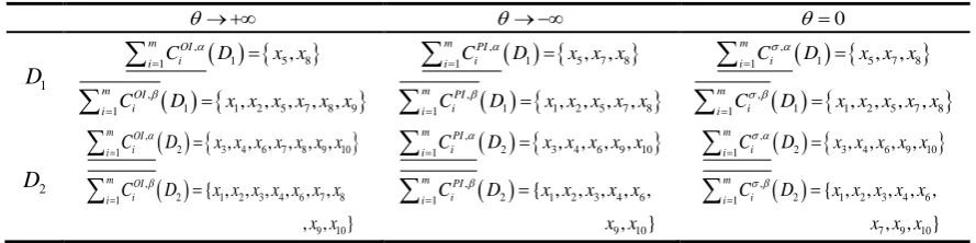
the definition of Sigmoid-multigranulation decision-theoretic rough set, the lower and upper approximation of D1 and D2 when   ,   and 0 are given in the Table 7,

respectively.

Table 3. The lower and upper approximation of D1 and D2 when  ,   and 0.

    0

1 D

   

,

1 5 8

1

,

1 1 2 5 7 8 9

1

,

, , , , ,

m _OI i i

m OI i i

C D x x

C D x x x x x x









   

,

1 5 7 8

1

,

1 1 2 5 7 8

1

, ,

, , , ,

m _PI i i

m PI i i

C D x x x

C D x x x x x









   

,

1 5 7 8

1

,

1 1 2 5 7 8

1

, ,

, , , ,

m i i

C D x x x

C D x x x x x

 

 





2 D

   

  ,

2 3 4 6 7 8 9 10

1

,

2 1 2 3 4 6 7 8

1

9 10 , , , , , ,

{ , , , , , ,

, , }

m OI i i

C D x x x x x x x

x x









   

  ,

2 3 4 6 9 10

1

,

2 1 2 3 4 6

1

9 10

, , , ,

{ , , , , ,

, }

m PI i i

C D x x x x x

x x









   

  ,

2 3 4 6 9 10

1

,

2 1 2 3 4 6

1

7 9 10 , , , ,

{ , , , , ,

, , }

m i i

C D x x x x x

x x x

 

 





By using three-way decision theory, we have the following decision rules:

(1) If the object x belongs to the lower of D1 or the complementary set of D2’s upper,

then the decision attribute value of x is 1;

(2) If the object x belongs to the lower of D2 or the complementary set of D1’s upper, then the

decision attribute value of x is 2; (3) Others are non-committed.

Therefore, we can get the following results when  :

The decision attribute value of x5 is 1;The decision attribute value of x3，x4，x6，x7，x9，x10

is 2;The objects x1，x2，x8 are non-committed.

[image:7.595.75.520.509.620.2]

(8)

The decision attribute value of x5, x7, x8 is 1;The decision attribute value of x3, x4, x6, x9,

10

x

is 2;The objects x1, x2 are non-committed.

When 0, the rules are:

The decision attribute value of x5, x7, x8 is 1;The decision attribute value of x3, x4, x6, x9,

10

x is 2;The objectsx₁, x₂ are non-committed.

Conclusion

This paper studies multigranulation decision-theoretic rough set in an incomplete interval-valued information system. We propose the notion of attribute similarity, and based the notion we define the maximal consistent class. In incomplete interval-valued information system, we can’t describe objects by equivalence class, therefore, we replace equivalence class with maximal consistent class when we establish multigranulation decision-theoretic rough set. In this paper, we propose Sigmoid-multigranulation decision-theoretic rough set based on Sigmoid function. Then, with the research for decision function, we propose generalized multigranulation decision-theoretic rough set. Finally, we illustrate that the models of multigranulation decision-theoretic rough set at present all can be covered by generalized multigranulation decision-theoretic rough set. In order to study the generalized multigranulation decision-theoretic rough set, we give the definition of decision function. Not only the parameter  which adjusting the different decision makers’ attitude to the risk is included, but also the parameters of t1, ,tl which affecting decision makers. But we don’t

research for the specific situation. Therefore, in the further work, the research for some type of decision makers is meaningful.

Acknowledgments

This work is supported by the National Natural Science Foundation of China (No. 61703426), National Natural Science Foundation of China (No. 61273275) and National Natural Science Foundation of China (No.61272011).

References

[1] Pawlak, Z. (1982). Rough set. International Journal of Computer & Information Sciences 11(5). [2] Liao, S. H., & Chen, Y. J. (2014). A rough set-based association rule approach implemented on exploring beverages product spectrum. Applied Intelligence,40(3), 464-478.

[3] Guo, Y., Jiao, L., Wang, S., Wang, S., Liu, F., & Rong, K., et al. (2015). A novel dynamic rough subspace based selective ensemble. Pattern Recognition,48(5), 1638–1652.

[4] Jensen, R., Tuson, A., & Shen, Q. (2014). Finding rough and fuzzy-rough set reducts with sat. Information Sciences,255, 100-120.

[5] Park, Y., & Kellis, M. (2015). Deep learning for regulatory genomics. Nature Biotechnology,33(8), 825-6.

[6] Qian, Y., Liang, J., Yao, Y., (2010). MGRS: A multi-granulation rough set. Information Sciences,180(6), 949-970.

[7] Xu, W., Zhang, X., & Wang, Q. (2011). A Generalized Multi-granulation Rough Set Approach. Bio-Inspired Computing and Applications—7th International Conference on Intelligent Computing, ICIC 2011, Zhengzhou, China, August 11-14. 2011, Revised Selected Papers (Vol. 6840, pp. 681-689).

(9)

[9] Jia, X., Tang, Z., Liao, W., & Shang, L. (2014). On an optimization representation of decision-theoretic rough set model. International Journal of Approximate Reasoning, 55(1), 156-166.

[10] Wojciech Ziarko. (2005). Probabilistic Rough Sets. Rough Sets, Fuzzy Sets, Data Mining, and Granular Computing, International Conference, Rsfdgrc 2005, Regina, Canada, August 31 - September 3, 2005, Proceedings (Vol. 3641, pp. 283-293).

[11] Ziarko, W. (1993). Variable precision rough set model. Journal of Computer & System Sciences,46(1)

[12] He, Q., Wu, C., Chen, D., & Zhao, S. (2011). Fuzzy rough set based attribute reduction for information systems with fuzzy decisions. Knowledge-Based Systems,24(5), 689-696.

[13] Lin, R. (2007). Upper and lower approximations based on intuitional fuzzy rough sets. Journal of Zhejiang Shuren University.

[14] Wei, D. K., & Zhou, X. Z. (2005). Rough set model in incomplete and fuzzy decision information system based on improved-tolerance relation. IEEE International Conference on Granular Computing (Vol.26, pp.647-57). IEEE.

[15] Zhou, X., & Li, H. (2009). A Multi-View Decision Model Based on Decision-Theoretic Rough Set. International Conference on Rough Sets and Knowledge Technology (Vol. 5589, pp. 650-657). Springer-Verlag.

[16] Yang, X., & Yao, J. (2010). A multi-agent decision-theoretic rough set model. Lecture Notes in Computer Science,6401(1), 711-718.

[17] Li, W., Huang, Z., Jia, X., & Cai, X. (2016). Neighborhood based decision-theoretic rough set models. International Journal of Approximate Reasoning,69, 1-17.

[18] Liang, D., Liu, D. (2015). Deriving three-way decisions from intuitionistic fuzzy decision-theoretic rough sets. Information Sciences, 300, 28-48.

[19] Li, H., Zhou, X., Zhao, J., & Liu, D. (2011). Attribute Reduction in Decision-Theoretic Rough Set Model: A Further Investigation. Rough Sets and Knowledge Technology, International Conference, Rskt 2011, Banff, Canada, October 9-12, 2011. Proceedings (Vol. 6954, pp. 466-475). [20] Liao, S., Zhu, Q., & Min, F. (2014). Cost-sensitive attribute reduction in decision-theoretic rough set models. Mathematical Problems in Engineering,2014(2), 1-9.

[21] Ma, X., Wang, G., Yu, H., & Li, T. (2014). Decision region distribution preservation reduction in decision-theoretic rough set model. Information Sciences,278, 614-640.

[22] Chen, H., Li, T., Luo, C., & Horng, S. (2015). A decision-theoretic rough set approach for dynamic data mining. IEEE Transactions on Fuzzy Systems,23(6), 1-1.

[23] Li, H., & Zhou, X. (2013). Risk decision making based on decision-theoretic rough set: a three-way view decision model. International Journal of Computational Intelligence Systems,4(1), 1-11.