Dimensionality Reduction for Time Series Decoding and Forecasting Problems

2018 IX International Conference on Optimization and Applications (OPTIMA 2018) ISBN: 978-1-60595-587-2

Dimensionality Reduction for Time Series Decoding and Forecasting

Problems

Roman ISACHENKO

, Mariia VLADIMIROVA

, and Vadim STRIJOV

Moscow Institute of Physics and Technology, Institutsky l. 9, 141701 Dolgoprudny Russia A. A. Dorodnicyn Computing Centre, Federal Research Center “Computer Science and Control” of the

Russian Academy of Sciences, Vavilova st. 40, 119333 Moscow, Russia Corresponding author

Keywords: Time series decoding, Forecast, Partial least squares, Dimensionality reduction

Abstract. _{The paper is devoted to the problem of decoding multiscaled time series and forecasting.}

The goal is to recover the dependence between an input signal and a target response. The proposed method allows receiving the predicted values not for the next timestamp but for the whole range of values in forecast horizon. The prediction is a multidimensional target vector instead of one timestamp point. We consider the linear model of partial least squares (PLS). The method finds the matrix of a joint description for the design matrix and the outcome matrix. The obtained latent space of the joint descriptions is low-dimensional. This leads to a simple, stable predictive model. We conducted computational experiments on the real dataset of energy consumption and electrocorticograms signals (ECoG). The experiments show significant reduction of the original spaces dimensionality, while the models achieve good prediction quality.

Introduction

The paper investigates the problem of dependence recovering between an input data and a model outcome. The proposed model is suitable for predicting a multidimensional target variable. In the case of the forecasting problem, objects and target spaces have the same nature. To build the model, we need to construct autoregressive matrices for input objects and target variables. The object is a local signal history, the outcome is signal values in the next timestamps. An autoregressive model makes an assumption that the current signal values depend linearly on the previous signal values.

In the case of time series decoding problem, objects and target spaces are different in nature, the outcome is a system response to the input signal. The autoregressive design matrix contains the local history of the input signal. The autoregressive target matrix contains the local history of the response.

The object space in time series decoding problems is high dimensional. Excessive dimensionality of the feature description leads to instability of the model. To solve this problem the feature selection procedures are used [13, 14].

The paper considers the partial least squares regression (PLS) model [22, 1, 9]. The PLS model reduces the dimensionality of the input data and extracts the linear combination of features which have the greatest impact on the response vector. Feature extraction is an iterative process in order of decreasing the influence on the response vector. PLS regression methods are described in details

1 2

*

in [8, 11, 4]. The difference between various PLS approaches, different kinds of PLS regression could be found in [21].

The current state of the field and the overview of nonlinear PLS method modifications are described in [20]. A nonlinear PLS method extension was introduced in [23]. There has been developed the variety of PLS modifications. The proposed nonlinear PLS methods are based on smoothing splines [6], neural networks [19], radial basis functions [24], genetic algorithms [10].

The result of the feature selection is the dimensionality reduction and the increasing model stability without significant loss of the prediction quality. The proposed method is used on two datasets with the redundant input and target spaces. The first dataset consists of hourly time series of energy consumption. Time series were collected in Poland from 1999 to 2004.

The second dataset comes from the NeuroTycho project [12] that designs bracomputer in-terface (BCI) [17, 15] for information transmitting between brains and electronic devices. Brain-Computer Interface (BCI) system enhances its user’s mental and physical abilities, providing a direct communication mean between the brain and a computer [16]. BCIs aim at restoring dam-aged functionality of motorically or cognitively impaired patients. The goal of motor imagery analysis is to recognize intended movements from the recorded brain activity. While there are various techniques for measuring cortical data for BCI [18, 2], we concentrate on the ElectroCor-ticoGraphic (ECoG) signals [5]. ECoG, as well as other invasive techniques, provides more stable recordings and better resolution in temporal and spatial domains than its non-invasive counter-parts. We address the problem of continuous hand trajectory reconstruction. The subdural ECoG signals are measured across 32 channels as the subject is moving its hand. Once the ECoG signals are transformed into informative features, the problem of trajectory reconstruction is the autore-gression problem. Feature extraction involves the application of some spectrotemporal transform to the ECoG signals from each channel [7].

In papers, which are devoted to forecasting of complex spatial time series, the forecast is built point-wise [3, 25]. If one needs to predict multiple points simultaneously, it is proposed to compute forecasted points sequentially. During this process, the previously predicted values are used to obtain subsequent ones. The proposed method allows obtaining multiple predicted time series values at the same time taking into account hidden dependencies not only in the object space but also in the target space. The proposed method significantly reduces the dimensionality of the feature space.

The main contributions of this paper are as follows:

ˆ addressing the dimensionality reduction problem for high-dimensional time series data,

ˆ significant reducing the dimensionality by introducing the latent space,

ˆ conducting computational experiments for real datasets with analysis of the results.

The rest of the paper is organized as follows. Section 2 states the problem of time series forecasting as optimization problem. Section 3 describes the PLS regression model in details. Section 4 is devoted to the computational experiments.

Problem Statement

Given a datasetD= (X,Y), whereX_∈Rm×n _{is a design matrix,Y ∈}

Rm×ris a target matrix.

The examples of how to construct the dataset for a particular application task are described in Section 4.

We assume that there is a linear dependence between the objects x _{∈ R}n _{and the responses}

y_∈Rr

y 1×r

= x 1×n·

Θ n×r

+ ε

1×r

, (1)

where Θis a matrix of model parameters, ε is a vector of residuals.

The task is to find the model parameter matrixΘgiven the datasetD. The optimal parameters are determined by error function minimization. Define a quadratic error functionS for the dataset

D:

S(Θ|D) =

X m×n·

Θ n×r−

Y m×r

2 2 = m X i=1 xi 1×n·

Θ n×r−

yi 1×r

2 2 →min

Θ . (2)

The linear dependence of the columns of the matrix X leads to an instable solution for the optimization problem (2). To avoid the strong linear dependence one could use feature selection techniques.

Partial Least Squares Method

To eliminate the linear dependence and reduce the dimensionality of the input space, principal components analysis (PCA) is widely used. The main disadvantage of the PCA method is its insensitivity to the interrelation between the objects and responses. The partial least squares algorithm projects the design matrix X and the target matrix Y to the latent space Rl with low

dimensionality (l < r < n). The PLS algorithm finds the latent space matrix T_∈Rm×l _{that best}

describes the original matrices X and Y.

The design matrixXand the target matrixYare projected into the latent space in the following way:

X m×n

= T m×l·

PT

l×n

+ F m×n

=

l X

k=1 tk m×1·

pTk

1×n

+ F m×n

, (3)

Y m×r

= T m×l·

QT

l×r

+ E m×r

=

l X

k=1 tk m×1·

qT_k

1×r

+ E m×r

, (4)

where T is a matrix of a joint description of the objects and outcomes in the latent space, and the columns of the matrix T are orthogonal; P, Q are transition matrices from the latent space to the original space; E, Fare residual matrices.

The pseudo-code of the PLS regression algorithm is given in Algorithm 1. In each of the l

steps the algorithm iteratively calculates columnstk,pk,qk of the matricesT,P,Q, respectively. After the computation of the next set of vectors, the one-rank approximations are subtracted from the matrices X, Y. This step is called a matrix deflation. In the first step, one has to normalize the columns of the original matrices (subtract the mean and divide by the standard deviation). During the test mode we need to normalize the test data, compute the model prediction (1), and then perform the reverse normalization.

The vectorstk anduk from the inner loop of Algorithm 1 contain information about the object matrix X and the outcome matrix Y, respectively. The blocks of steps (6)–(7) and (8)–(9) are analogs of the PCA algorithm for the matrices X and Y [9]. Sequential repetition of the blocks takes into account the interaction between the matrices X and Y.

The theoretical explanation of the PLS algorithm follows from the following statements.

Algorithm 1. PLSR algorithm

Require: X,Y, l;

Ensure: T,P,Q;

1: normalize matrices X Y by columns 2: initialize u0 (the first column of Y)

3: X1 =X;Y1 =Y

4: for k = 1, . . . , l do

5: repeat

6: wk:=XT_kuk−1/(u

T

k−1uk−1); wk := _kwwk kk

7: tk :=Xkwk

8: ck :=Y_kTtk/(tT_ktk); ck := ck kckk

9: uk :=Ykck

10: until tk stabilizes

11: pk:=XT_ktk/(tT_ktk), qk :=YT_ktk/(tT_ktk)

12: Xk+1 :=Xk−tkp

T

k

13: Yk+1 :=Yk−tkq

T

k

14: end for

Assertion 1.The best description of the matricesXandY taking into account their interrelation

is achieved by maximization the covariance between the vectors tk and uk.

Proof. The statement follows from the equation

cov(tk,uk) = corr(tk,uk)·pvar(tk)·pvar(uk).

Maximization of variances of the vectors tk and uk corresponds to keeping information about original matrices, the correlation of these vectors corresponds to interrelation between X and Y.

In the inner loop of Algorithm 1 the normalized weight vectorswkandckare calculated. These vectors construct the matrices W and C, respectively.

Assertion 2.The vectorwkandck are eigenvectors of the matricesXT_kYkY_kTXkandYT_kXkXT_kYk,

corresponding to the maximum eigenvalues.

wk ∝XT_kuk−1 ∝X

T

kYkck−1 ∝X

T

kYkY

T

ktk−1 ∝X

T

kYkY

T

kXkwk−1,

ck ∝YT_ktk ∝Y_kTXkwk ∝Y_kTXkXT_kuk−1 ∝Y

T

kXkX

T

kYkck−1,

where the ∝ symbol means equality up to a multiplicative constant.

Proof. The statement follows from the fact that the update rule for vectors wk,ck coincides with

the iteration of the power method for the maximum eigenvalue. Let a matrix A be diagonalizable, xbe some vector, then

lim

k→∞A k

x=λmax(A)·vmax,

where λmax(A) is the maximum eigenvalue of the matrix A, vmax is the eigenvector of the matrix A, corresponding to λmax(A).

Assertion 3. The update rule for the vectors in steps (6)–(9) of Algorithm 1 corresponds to the

maximization of the covariance between the vectors tk and uk.

Proof. The maximum covariance between the vectors tk and uk is equal to the maximum

eigen-value of the matrix XT_kYkYT_kXk:

max

tk,ukcov(tk,uk)

2 _{= max} kwkk=1

kckk=1

cov (Xkwk,Ykck)2 = max

kwkk=1 kckk=1

covcT_kYT_kXkwk2 =

= max

kwkk=1cov Y

T

kXkwk 2

= max

kwkk=1w

T

kX

T

kYkY

T

kXkwk =

=λmax

XT_kYkY_kTXk,

where λmax(A) is the maximum eigenvalue of the matrix A. Using Statement 2, we obtain the

required result.

After the inner loop, the step (11) is to compute vectors pk, qk by projection of the columns of the matricesXk and Yk to the vector tk. To go to the next step one has to deflate the matrices

Xk and Yk by the one-rank approximations tkpTk and tkq

T

k

Xk+1 =Xk−tkp

T

k =X− X

k

tkpTk,

Yk+1 =Yk−tkq

T

k =Y− X

k

tkqT_k.

Each next vector tk+1 turns out to be orthogonal to all vectors ti, i= 1, . . . , k.

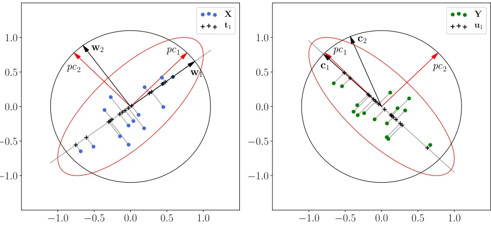
Let us assume that the dimension of object, response and latent variable spaces are equal to 2 (n = r = l = 2). Fig. 1 shows the result of the PLS algorithm in this case. Blue and green dots represent the rows of the matrices Xand Y, respectively. The dots were generated from a normal distribution with zero expectation. Contours of the distribution covariance matrices are shown in red. Black contours are unit circles. Red arrows correspond to principal components for the set of points. Black arrows correspond to the vectors of the matrices W and C from the PLS algorithm. The vectorstk anduk are equal to the projected matricesXk andYk to the vectorswk

andck, respectively, and are denoted by black pluses. Taking into account the interaction between the matrices X and Y the vectors wk and ck deviates from the principal components directions. The deviation of the vectors wk is insignificant. In the first iteration, c1 is close to the principal

component pc1, but the vectors ck in the next iterations could strongly correlate. The difference

in the behavior of the vectorswk andck is associated with the deflation process. In particular, we subtract from Y the one-rank approximation found in the space of the matrix X.

To obtain the model predictions and find the model parameters, let us multiply both hand sides of the equation (3) by the matrix W. Since the rows of the residual matrixEare orthogonal to the columns of the matrixW, we have

XW=TPTW.

−1.0 ₋0.5 0.0 0.5 1.0 −1.0

−0.5 0.0 0.5 1.0

w1

pc1 w2

pc2

X t1

−1.0 ₋0.5 0.0 0.5 1.0 −1.0

−0.5 0.0 0.5

1.0 c2

pc2 c1

pc1

Y u1

Figure 1. The result of the PLS algorithm for the case n=r=l = 2.

The linear transformation between objects in the input and latent spaces has the form

T=XW∗, (5)

where W∗ _=W(PT

W)−1_.

The matrix of the model parameters 1 could be found from equations (4), (5)

Y=TQT +E=XW∗_QT

+E=XΘ+E.

Thus, the model parameters (1) are equal to

Θ=W(PTW)−1_QT

. (6)

To find the model predictions during the testing, we have to

ˆ normalize the test data;

ˆ compute the prediction of the model using the linear transformation with the matrix Θ

from (6);

ˆ perform the inverse normalization.

Computational Experiment

All computational experiments were conducted using a personal laptop with 2.3 GHz. We use Matlab and Python as the main programming languages for the analysis.

Time series of energy consumption contain hourly records (total of 52512 observations). A row of the matrix X is the local history of the signal for one week n= 24×7. A row of the matrix Y

is the local forecast of energy consumption for the next 24 hoursr= 24. In this case, the matrices

X and Y are autoregressive matrices.

0 50 100 150 200 250 300 Time, ms

ch 4 ch 3 ch 2 ch 1

100 150 200 250 300 220 260

300 340₃₈₀ 50

100 150 200

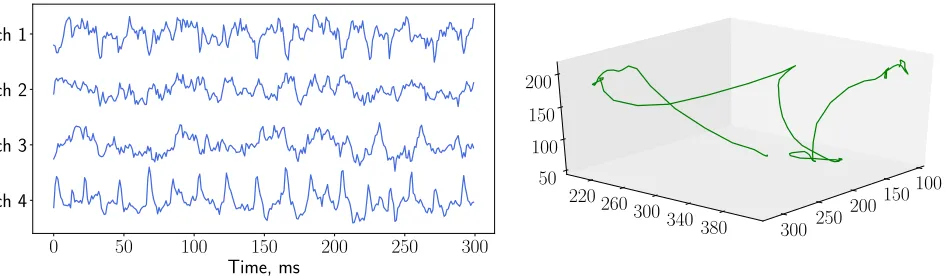
Figure 2. The ECoG data example. On the left the voltage data taken from multiple channels is shown, on the right there are coordinates of the hand along three axes.

In the case of the ECoG data, the matrix X consists of the spatial-temporal representation of voltage time series, and the matrix Y contains information about the position of the hand. The generation process of the matrix X from the voltage values described in [7]. Feature description in each time moment has dimension equal to 864. The hand position is described by the coordi-nates along three axes. An example of voltage data samples with the different channels and the corresponding spatial coordinates of the hand are shown in Fig. 2. To predict the position of the hand in the next moments we used an autoregressive approach. One object consists of a feature description in a few moments. The answer is the hand position in the next moments of time. The task is to predict the hand position in the next few moments of time.

We introduce the mean-squared error for matrices A= [aij] andB = [bij]

MSE(A,B) =X

i,j

(aij −bij)2.

To estimate the prediction quality, we compute the normalized MSE

NMSE(Y,Yˆ) = MSE(Y,Yˆ)

MSE(Y,Y¯), (7)

whereYˆ is the model outcome, Y¯ is the average constant forecast over the columns of the matrix.

Energy Consumption Dataset

To find the optimal dimensionality l of the latent space, the energy consumption dataset was divided into training and validation parts. The training data consists of 700 objects, the validation data is of 370 ones. The dependence of the normalized mean-squared error (7) on the latent space with dimensionality l is shown in Fig. 3. First, the error drops sharply with increasing the latent space dimensionality and then changes slightly.

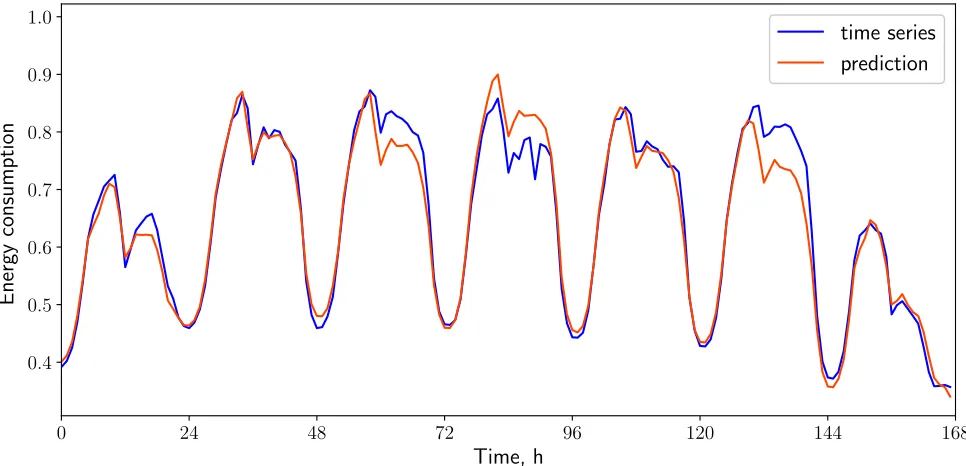
The error achieves the minimum value forl = 14. Let us build a forecast of energy consumption for a given l. The result is shown in Fig. 4. The PLS algorithm restored the autoregressive dependence and found the daily seasonality.

0 5 10 15 20

Number of PLS components,l

0.1 0.2 0.3

N

M

S

E

Figure 3. NMSE as a function of dimension l of latent space for energy consumption data.

0 24 48 72 96 120 144 168

Time, h 0.4

0.5 0.6 0.7 0.8 0.9 1.0

E

ne

rg

y

co

ns

um

pt

io

n

time series prediction

Figure 4. The energy consumption forecast by the PLS algorithm (the latent space dimensionality is equal tol = 14).

ECoG Dataset

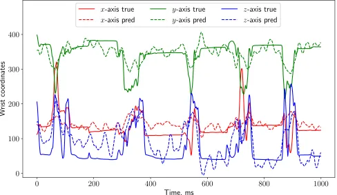
Fig. 5 illustrates the dependence of the normalized mean-squared error (7) on the latent space dimensionality l for ECoG dataset. The approximation error changes slightly forl >5. The joint spatial-temporal representation of objects and the position of the hand can be represented as a vector of dimensionality equal to l n. Let us fixl = 5. An example of the approximation of the hand position is shown in Fig. 6. Solid lines represent the true coordinates of the hand along all axes, the dotted lines show the approximation by the PLS algorithm.

0 5 10 15 20

Number of PLS components,l

0.7 0.8 0.9

N

M

S

E

Figure 5. NMSE as a function of dimension l of latent space for the ECoG data.

0 200 400 600 800 1000

Time, ms

0 100 200 300 400

W

ri

st

co

or

di

na

te

s

x-axis true x-axis pred

y-axis true y-axis pred

z-axis true z-axis pred

Figure 6. The hand motions predicted by the PLS algorithm (the latent space dimensionality is equal to l= 5).

Conclusion

In the paper, we proposed the approach for solving the problem of time series decoding and forecasting. The algorithm of partial least squares allows building a simple, stable and linear

model. The obtained latent space gathers information about the objects and the responses and dramatically reduces the dimensionality of the input matrices. The computational experiment demonstrated the applicability of the proposed method to the tasks of electricity consumption forecasting and brain-computer interface designing. The future research will be aimed at the extension of the proposed method for the class of non-linear dependencies.

Acknowledgements

This research was supported by Russian Science Foundation, grand no. 16-07-01155 and the Government of the Russian Federation, agreement 05.Y09.21.0018.

References

[1] Herv´e Abdi. Partial Least Squares (PLS) Regression. Encyclopedia for research methods for the social sciences, pages 792–795, 2003.

[2] Setare Amiri, Reza Fazel-Rezai, and Vahid Asadpour. A review of hybrid brain-computer interface systems. Advances in Human-Computer Interaction, 2013:1, 2013.

[3] George EP Box, Gwilym M Jenkins, Gregory C Reinsel, and Greta M Ljung. Time series analysis: forecasting and control. John Wiley & Sons, 2015.

[4] Sijmen De Jong. Simpls: an alternative approach to partial least squares regression. Chemo-metrics and intelligent laboratory systems, 18(3):251–263, 1993.

[5] Andrey Eliseyev and Tetiana Aksenova. Penalized multi-way partial least squares for smooth trajectory decoding from electrocorticographic (ecog) recording. PloS one, 11(5):e0154878, 2016.

[6] Ildiko E. Frank. A nonlinear PLS model. Chemometrics and Intelligent Laboratory Systems, 8(2):109–119, 1990.

[7] Motrenko A. Gasanov I. Creation of approximating scalogram description in a problem of movement prediction. Journal of Machine Learning and Data Analysis, 3(2):160–169, 2017. [8] Paul Geladi. Notes on the history and nature of partial least squares (PLS) modelling. Journal

of Chemometrics, 2(January):231–246, 1988.

[9] Paul Geladi and Bruce R Kowalski. Partial least-squares regression: a tutorial. Analytica chimica acta, 185:1–17, 1986.

[10] Hugo Hiden, Ben McKay, Mark Willis, and Gary Montague. Non-linear partial least squares using genetic. InGenetic Programming 1998: Proceedings of the Third, pages 128–133. Morgan Kaufmann, 1998.

[11] Agnar H¨oskuldsson. PLS regression.Journal of Chemometrics, 2(August 1987):581–591, 1988. [12] Project Tycho http://neurotycho.org/food-tracking-task.

[13] AM Katrutsa and VV Strijov. Stress test procedure for feature selection algorithms. Chemo-metrics and Intelligent Laboratory Systems, 142:172–183, 2015.

[14] Jundong Li, Kewei Cheng, Suhang Wang, Fred Morstatter, Robert P Trevino, Jiliang Tang, and Huan Liu. Feature selection: A data perspective. arXiv preprint arXiv:1601.07996, 2016. [15] SG Mason, A Bashashati, M Fatourechi, KF Navarro, and GE Birch. A comprehensive survey of brain interface technology designs. Annals of biomedical engineering, 35(2):137–169, 2007. [16] Jos´e del R Mill´an, Fr´ed´eric Renkens, Josep Mouri˜no, and Wulfram Gerstner. Brain-actuated

interaction. Artificial Intelligence, 159(1-2):241–259, 2004.

[17] Jos´e del R Mill´an, R¨udiger Rupp, Gernot Mueller-Putz, Roderick Murray-Smith, Claudio Giugliemma, Michael Tangermann, Carmen Vidaurre, Febo Cincotti, Andrea Kubler, Robert Leeb, et al. Combining brain–computer interfaces and assistive technologies: State-of-the-art and challenges. Frontiers in Neuroscience, 4:161, 2010.

[18] Luis Fernando Nicolas-Alonso and Jaime Gomez-Gil. Brain computer interfaces, a review.

Sensors, 12(2):1211–1279, 2012.

[19] S Joe Qin and Thomas J McAvoy. Nonlinear pls modeling using neural networks. Computers & Chemical Engineering, 16(4):379–391, 1992.

[20] Roman Rosipal. Nonlinear partial least squares: An overview. Chemoinformatics and Ad-vanced Machine Learning Perspectives: Complex Computational Methods and Collaborative Techniques, pages 169–189, 2011.

[21] Roman Rosipal and Nicole Kramer. Overview and Recent Advances in Partial Least Squares.

C. Saunders et al. (Eds.): SLSFS 2005, LNCS 3940, pages 34–51, 2006.

[22] Jacob A Wegelin et al. A survey of partial least squares (pls) methods, with emphasis on the two-block case. University of Washington, Department of Statistics, Tech. Rep, 2000.

[23] Svante Wold, Nouna Kettaneh-Wold, and Bert Skagerberg. Nonlinear pls modeling. Chemo-metrics and Intelligent Laboratory Systems, 7(1-2):53–65, 1989.

[24] Xuefeng F. Yan, Dezhao Z. Chen, and Shangxu X. Hu. Chaos-genetic algorithms for optimizing the operating conditions based on RBF-PLS model. Computers and Chemical Engineering, 27(10):1393–1404, 2003.

[25] G Peter Zhang. Time series forecasting using a hybrid arima and neural network model.

Neurocomputing, 50:159–175, 2003.