A difference based approach in the partially linear model with dependent errors

R E S E A R C H

Open Access

A difference-based approach in the

partially linear model with dependent errors

Zhen Zeng

_{and Xiangdong Liu}

*_{Correspondence:}

[email protected]; [email protected]

1_{Department of Statistics, Jinan}

University, Guangzhou, P.R. China

Abstract

We study asymptotic properties of estimators of parameter and non-parameter in a partially linear model in which errors are dependent. Using a difference-based and ordinary least square (DOLS) method, the estimator of an unknown parametric component is given and the asymptotic normality of the DOLS estimator is obtained. Meanwhile, the estimator of a nonparametric component is derived by the wavelet method, and asymptotic normality and the weak convergence rate of the wavelet estimator are discussed. Finally, the performance of the proposed estimator is evaluated by a simulation study.

MSC: 62G05; 62G20

Keywords: NSD random variables; Partially linear model; Asymptotic normality; Finite difference; Least square

1 Introduction

Consider the partially linear model (PLM)

yi=xTi β+f(ti) +ei, 1≤i≤n, (1)

where the superscriptT denotes the transpose, yi are scalar response variables, xi=

(xi1, . . . ,xid)T are explanatory variables, β is a d-dimensional column vector of the

un-known parameter,f(·) is an unknown function,ti are deterministic with 0≤t1≤ · · · ≤ tn≤1, andeiare random errors.

PLM was first considered by Engle et al. [1], and now is one of the most widely used statistical models. It can be applied in almost every field, such as engineering, economics, medical sciences and ecology, etc. There are many authors (see [2–8]) concerned with var-ious estimation methods to obtain estimators of the unknown parameters and nonparam-eters for partially linear model. Deep results such as asymptotic normality of estimators have been obtained.

In this paper, by a difference-based approach, we will use the ordinary least square and wavelet to investigate model (1). The differencing procedures provide a convenient means for introducing nonparametric techniques to practitioners in a way which parallels their knowledge of parametric techniques, and differencing procedures may easily be combined with other procedures. For example, Wang et al. [9] obtained a difference-based approach to the semiparametric partially linear model. Tabakan et al. [10] studied a difference-based

ridge in partially linear model. Duran et al. [11] investigated the difference-based ridge and Liu type estimators in semiparametric regression models. Hu et al. [12] used a difference-based Huber Dutter estimator (DHD) to obtain the root varianceσand parametricβfor partially linear model. Wu [13] constructed the restricted difference-based Liu estima-tor for the parametric component of partially linear model. However, in the majority of the previous work it is assumed that errors are independent. The asymptotic problem of difference-based estimators of partially linear model with dependent errors is in practice important. In this paper, we use a difference-based and ordinary least square method to study the partially linear model with dependent errors.

For the dependent errorseiwe confine ourselves to negatively superadditive dependent

(NSD) random variables. There are many applications of NSD random variables in multi-variate statistical analysis; see [14–23]. Hence, it is meaningful to study the properties of NSD random variables. The formal definition of NSD random variables is the following.

Definition 1(Kemperman [24]) A function: Rn_{→Ris called superadditive if(x∨} y) +(x∧y)≥(x) +(y) for allx,y∈Rn_{, where∨stands for componentwise maximum,}

and∧for componentwise minimum.

Definition 2(Hu [25]) A sequence{e1,e2, . . . ,en}is said to be NSD if

E(e1,e2, . . . ,en)≤E(Y1,Y2, . . . ,Yn), (2)

whereY1,Y2, . . . ,Ynare independent withei=dYifor eachi, andis a superadditive

func-tion such that the expectafunc-tions in (2) exist. An infinite sequence{en,n≥1} of random

variables is said to be NSD if{e1,e2, . . . ,en}is NSD for alln≥1.

In addition, using the wavelet method (see [26–29]), the weak convergence rate and asymptotic normality of the estimator off(·) are obtained.

Throughout the paper we fix the following notations.β0is the true value of the unknown

parameterβ. Z is the set of integers, N is the set of natural numbers, R is the set of real numbers. Denotex+_{=max(x, 0), andx}–_{= (–x)}+_{. LetC1,C2,C3,C4are positive constants.}

For a sequence of random variablesηnand a positive sequencedn, writeηn=o(dn) ifηn/dn

converges to 0 andηn=O(dn) ifηn/dnis bounded. We can similarly define the notations

ofoP andOPfor stochastic convergence and stochastic bounded. Weak convergence of

a distribution is denoted by Hn D

→H, and for random variables byYn D

→Y.xis the Euclidean norm ofx, and x=max{k∈Z:k≤x}.

2 Estimation method

Define the (n–m)×ndifferencing matrixDas

D= ⎛ ⎜ ⎜ ⎜ ⎜ ⎜ ⎜ ⎜ ⎝

d0 d1 d2 · · · dm 0 · · · 0

0 d0 d1 d2 · · · dm 0 · · · 0

..

. ... ... ... ... ... ... ... ... ... ... ... 0 · · · 0 d0 d1 d2 · · · 0 0 · · · 0 d0 d1 d2 · · · dm

where the positive integer numbermis the order of differencing and d0,d1, . . . ,dm are

differencing weights satisfying

m

q=0 dq= 0,

m

q=0

d_q2= 1. (3)

This differencing matrix is given by Yatchew [30]. Using the differencing matrix to model (1), we have

DY=DXβ+Df+De. (4)

From Yatchew [30], the application of differencing matrixDin model (1) can remove the nonparametric effect in large samples, so we will ignore the presence ofDf. Thus, we can rewrite (4) as

˜

Y=Xβ˜ +˜e, (5)

where Y˜ = (y1˜ , . . . ,y˜n–m)T,X˜ = (x1˜ , . . . ,x˜n–m)T andn=X˜TX˜ is nonsingular for largen, ˜

e= (e1˜ , . . . ,e˜n–m)T,y˜i= mq=0dqyi+q,x˜i= mq=0dqxi+q,e˜i= qm=0dqei+q,i= 1, . . . ,n–m.

As a usual regression model, the ordinary least square estimator βˆnof the unknown

parameterβis given as

ˆ

βn=arg min

β

n–m

i=1

˜ yi–x˜Ti β

2

. (6)

Then the estimator satisfies

–2

n–m

i=1 ˜ xi

˜ yi–x˜Tiβˆn

= 0,

and hence

ˆ

βn=–1n X˜TY˜. (7)

In the following, we use wavelet techniques to estimatef(·) ifβˆnis known.

Suppose that there exists a scaling functionφ(·) in the Schwartz spaceSland a

multires-olution analysis{Vm˜}in the concomitant Hilbert spaceL2(R), with the reproducing kernel

Em˜(t,s) given by

Em˜(t,s) = 2m˜E0

2m˜t, 2m˜s= 2m˜

k∈Z

φ2m˜t–kφ2m˜s–k.

LetAi= [si–1,si] denote intervals that partition [0, 1] withti∈Aifor 1≤i≤n. Then the

estimator of the nonparameterf(t) is given by

ˆ fn(t) =

n

i=1

yi–xTiβˆn Ai

3 Preliminary conditions and lemmas

In this section, we give the following conditions and lemmas which will be used to obtain the main results.

(C1) max_1≤i≤nxi=C1<∞.

(C2) f(·)∈Hα_{(Sobolev space), for someα> 1/2.} (C3) f(·)is Lipschitz function of orderγ > 0.

(C4) φ(·)belongs toSl, which is a Schwartz space forl≥α.φ(·)is a Lipschitz function

of order 1 and has compact support, in addition to| ˆφ(ξ) – 1|=O(ξ)asξ→0, whereφˆdenotes Fourier transform ofφ.

(C5) si,1≤i≤n, satisfymax1≤i≤n(si–si–1) =O(n–1), and2m˜ =O(n1/3).

Remark3.1 Condition (C1) is standard and often imposed in the estimator of partial linear models, once can refer to Zhao et al. [31]. Conditions (C2)–(C5) are used by Hu et al. [29]. Therefore, our conditions are very mild and can easily be satisfied.

Lemma 3.1(Hu [25]) Suppose that{e1,e2, . . . ,en}is NSD.

(i) Ifg1,g2, . . . ,gnare nondecreasing functions,then{g1(e1),g2(e2), . . . ,gn(en)}is NSD.

(ii) For any2≤m≤nand1≤i1<i2<· · ·<im,{ei1,ei2, . . . ,eim}is NSD.

Lemma 3.2(Wang et al. [17]) Let p> 1.Let{en,n≥1}be a sequence of NSD random variables with Een= 0and E|en|p<∞for each n≥1.Then for all n≥1,

E

max

1≤k≤n

k

i=1 ei

p ≤23–p

n

i=1

E|ei|p for1 <p≤2 (9)

and

E

max

1≤k≤n

k

i=1 ei

p ≤2

15p

lnp

pn

i=1 E|ei|p+

_n

i=1 Ee2_i

p/2

for p> 2. (10)

Lemma 3.3 Let p> 1.Let{en,n≥1}be a sequence of NSD random variables with Een= 0 and E|en|p<∞for all n≥1,and{cq, 0≤q≤m}be a sequence of real constants.Then for all n≥1,

E

max

1≤k≤n–m

k

i=1 m

q=0 cqei+q

p

≤4mp–1 n

i=1 m

q=0

E|cqei+q|p for1 <p≤2 (11)

and,for p> 2,

E

max

1≤k≤n–m

k

i=1 m

q=0 cqei+q

p

(12)

≤2p+1mp–1

15p

lnp

pn

i=1 m

q=0

E|cqei+q|p+

_n

i=1 m

q=0

E(cqei+q)2

p/2

.

Proof Letz1i= mq=0c+qei+q,z2i= mq=0c–qei+q, then mq=0cqei+q=z1i–z2i, and{c+qei+q,i≥1}

and{c–

Cr-inequality,

E

max

1≤k≤n–m

k i=1 m q=0 cqei+q

p =E max

1≤k≤n–m

k i=1

(z1i–z2i)

p

≤2p–1

E

max

1≤k≤n–m

k i=1 z1i p +E max

1≤k≤n–m

k i=1 z2i p

≤2p–1mp–1 m q=0 E max

1≤k≤n–m

k i=1 c+_qei+q

p +E max

1≤k≤n–m

k i=1 c–_qei+q

p

.

In the case 1 <p≤2, it follows from Lemma3.2that

E

max

1≤k≤n–m

k k=1 m q=0 cqei+q

p

≤2p–1mp–1 m q=0 E max

1≤k≤n–m

k i=1 c+_qei+q

p +E max

1≤k≤n–m

k i=1 c–_qei+q

p

≤4mp–1

_n–m

i=1 m

q=0

Ec+_qei+qp+ n–m

i=1 m

q=0

Ec–_qei+qp

. (13)

Note that|cq|p=|c+q|p+|c–q|p, the desired result (11) follows from (13) immediately. In the

same way, we also have (12). The proof is completed.

Remark3.2 From Lemma3.3and Lemma3.1, we have, for 1 <p≤2,

E

i∈S m

q=0 cqei+q

p

≤4mp–1

i∈S m

q=0

E|cqei+q|p

(14)

and, forp> 2,

E

i∈S m

q=0 cqei+q

p

≤2p+1mp–1

15p

lnp

p

i∈S m

q=0

E|cqei+q|p+

i∈S m

q=0

E(cqei+q)2

p/2

, (15)

whereS⊂ {1, 2, . . . ,n}.

Lemma 3.4 Let A and B be disjoint subsets ofN,and{Xj,j∈A∪B}be a sequence of NSD random variables.Let f: R→Rand g: R→Rbe differentiable with bounded derivatives,

and · ∞stand for supnorm.Then

Cov

f

i∈A aiXi

,g

j∈A ajXj

≤f_∞g_∞Cov

i∈A aiXi,

j∈B ajXj

provided the covariation on the right hand side exists,where{ai, 1≤i≤n}is an array of real numbers.

Proof For a pair of random variablesZ1= _i∈AaiXi,Z2= j∈BajXj, we have

H(z1,z2) =P(Z1≤z1,Z2≤z2) –P(Z1≤z1)P(Z2≤z2).

Denote by F(z1,z2) the joint distribution functions of (Z1,Z2), and FZ1(z2),FZ2(z2) the marginal distribution function ofZ1,Z2, one gets

Cov(Z1,Z2) =E(Z1Z2) –E(Z1)E(Z2)

= F(z1,z2) –FZ1(z1)FZ2(z2)

dz1dz2= H(z1,z2)dz1dz2,

this relation was established in Lehmann [32] for any two random variablesZ1andZ2with Cov(Z1,Z2) exist. Letf,gare complex valued function on R with derivativesf,g<∞, then we have

Covf(Z1),g(Z2)

= f(Z1)g(Z2)H(z1,z2)dz1dz2

≤ f(Z1)g(Z2)H(z1,z2)dz1dz2≤f_∞g_∞Cov(Z1,Z2).

The proof is completed.

Lemma 3.5 Let{en,n≥1}be a sequence of NSD random variable with Een= 0.Let˜eij= m

q=0dqeij+q,and|ij–ik|>m if j=k.Then

Eexp

i

n

j=1 tije˜ij

–

n

j=1

Eexp(itije˜ij)

≤–

n

j=1 n

k=j+1 m

q1=0 m

q2=0

t₀2Cov(eij+q1,eik+q2), (16)

wherei =√–1, m_q=0dq= 0and mq=0d2q= 1,ti1,ti2, . . . ,tinare real numbers with|tij| ≤t0.

Proof Notice that the result is true forn= 1.

For n = 2, let f(˜ei1) = exp{iti1e˜i1},g(e˜i2) = exp{iti2˜ei2}. Then, by Lemma 3.4 and

m

q=0d2q= 1,

_Eexp{iti1˜ei1+ iti2˜ei2}–Eexp{iti1e˜i1}Eexp{iti2e˜i2}

=Covexp{iti1e˜i1},exp{iti2e˜i2}

≤t2₀

m

q1=0 m

q2=0

dq1dq2Cov(ei1+q1,ei2+q2)

≤–t2₀ m

q1=0 m

q2=0

Hence, the result is true forn= 2.

Moreover, suppose that (16) holds forn– 1. By Lemma3.4, we have, forn, Eexp i n j=1 tije˜ij

–

n

j=1

Eexp{itije˜ij}

≤Eexp

i

n

j=1 tije˜ij

–Eexp

i

n–1

j=1 tij˜eij

Eexp{itin˜ein}

+ Eexp i n–1 i=1 tij˜eij

Eexp{itin˜ein}– n–1

j=1

Eexp{itije˜ij}Eexp{itine˜in}

≤Cov exp i n–1 i=1 tije˜ij

,exp{itine˜in}

+ Eexp i n–1 j=1 tije˜ij

–

n–1

j=1

Eexp{itije˜ij}

≤Cov exp i n–1 i=1 tije˜ij

,exp{itine˜in}

+ n–1 j=1 n–1

k=j+1 m q1=0 m q2=0

t₀2Cov(eij+q1,eik+q2)

≤–t2 0 n j=1 n

k=j+1 m q1=0 m q2=0

Cov(eij+q1,eik+q2),

which completes the proof.

Lemma 3.6(Hu et al. [29]) If Condition(C3)holds,then

(a1) |E0(t,s)| ≤₍₁₊C_|t–k_s|)k,|Em˜(t,s)| ≤ 2

˜

m_C

(1+2m˜_|t–s|)k (wherek∈NandC=C(k)is a constant

depending onkonly).

(a2) sup_0≤s≤1|Em_˜(t,s)|=O(2m˜).

(a3) sup_t01|Em˜(t,s)|ds≤C2.

(a4) ₀1Em˜(t,s)ds→1,n→ ∞.

Lemma 3.7(Rao [33]) Suppose that{Xn,n≥1}are independent random variables with EXn= 0and s–(2+n δ) nj=1E|Xj|2+δ→0for someδ> 0.Then

s–1_n n

j=1 Xj

D

→N(0, 1),

where s2

n= nj=1EXj2=Var( n j=1Xj).

Lemma 3.8(Yu et al. [34]) Let{en,n≥1}be a sequence of NSD random variable satisfying Een= 0,supj≥1 i:|i–j|≥u|Cov(ei,ej)| →0as u→ ∞,and{ani, 1≤i≤n,n≥1}be an array of real numbers withmax1≤i≤n|ani| →0and ni=1a2ni=O(1).Suppose that{en,n≥1}is uniformly integral in L2,then

σ_n–1 n

i=1 aniei

D

→N(0, 1),

4 Main results and their proofs

Theorem 4.1 Under Condition(C1),suppose that{en,n≥1}is a sequence of NSD random variables with Een= 0and

(i) sup_n≥1E|en|2+δ<∞for someδ> 0,

(ii) sup_{j≥1 i:|i–j|≥u}|Cov(ei,ej)| →0asu→ ∞.Then

(n–m)–12_τ–1

β n(βˆn–β0) D

−→N(0,Id) (17)

provided that

τ_β2= lim

n→∞(n–m) –1

_n–m

i=1 ˜

xix˜Ti Var(˜ei) + 2 n–m

i=1 n–m

j=i+1 ˜

xix˜Tj Cov(˜ei,e˜j)

(18)

is a positive definite matrix,whereIdis the identity matrix of orderd.

Proof By Condition (i), we have

sup

n≥1

Ee2_n<∞ and lim

x→∞sup_n≥1Ee

2 nI

|en|>x

= 0,

from which it follows that

C3:=sup n>m

(n–m)–1

n–m

i=1 m

q=0

Var(dqei+q) <∞,

and for allε> 0

(n–m)–1

n–m

i=1 m

q=0

E(dqei+q)2I

|dqei+q| ≥ √

n–mε→0 asn→ ∞.

Then we can find a positive number sequence{εn,n≥1}withεn→0 such that

(n–m)–1

n–m

i=1 m

q=0

E(dqei+q)2I

|dqei+q| ≥ √

n–mεn

→0 asn→ ∞.

Now, we define the integers:m0= 0, and, for eachj= 0, 1, 2, . . . , put

m2j+1=min

m:m≥m2j, (n–m)–1 m

i=m2j+1

m

q=0

Var(dqei+q) >√εn

,

m2j+2=m2j+1+

1

εn

+m.

Denote

Ij={k:m2j<k≤m2j+1,j= 0, . . . ,l} and

wherel=l(n) is the number of blocks of indicesIj. Then

l√εn≤(n–m)–1 l

j=1

i∈Ij m

q=0

Var(dqei+q)≤(n–m)–1 n–m

i=1 m

q=0

E(dqei+q)2≤C3, (19)

and hence we havel≤C3/√εn. If the number of the remainder term is not zero when the

construction ends, then we put all the remainder terms into a block denoted byJl. By (7),

we have

n(βˆn–β0) = n–m

i=1 ˜

xie˜i. (20)

Then to prove (17), it is enough to prove that

(n–m)–1/2τ_β–1 n–m

i=1 ˜ xie˜i

D

→N(0,Id). (21)

Letube an arbitraryd-dimensional column vector withu= 1, and setai=uTτβ–1x˜i.

Then, by the Cramér–Wold device, to prove (21) it suffices to prove that

1

√ n–m

n–m

i=1 aie˜i

D

→N(0, 1). (22)

Write

1

√ n–m

n–m

i=1 aie˜i=

1

√ n–m

l

j=1

i∈Ij aie˜i+

1

√ n–m

l

j=1

i∈Jj aie˜i

:=I+J.

Moreover, note thatmax0≤q≤m|dq| ≤1 andmax1≤i≤n|ai|<∞by Condition (C1), then

applying Lemma3.3withp= 2 we have

E

1

√ n–m

l

j=1

i∈Jj ai˜ei

2

= 1

n–mE

_l

j=1

i∈Jj m

q=0 aidqei+q

2

≤ 4m n–m

l

j=1

i∈Jj m

q=0

E|aidqei+q|2

≤ 4m n–m

! max

m1≤i≤m2l+2

a2_i

"l

j=1

i∈Jj m

q=0

E|dqei+q|2

≤ 4m n–m

! max

m1≤i≤m2l+2

a2_i

"l

j=1

i∈Jj m

q=0

E|dqei+q|2I

|dqei+q| ≥ √

n–mεn

+ 4m

n–m

! max

m1≤i≤m2l+2

a2_i

"l

j=1

i∈Jj m

q=0

E|dqei+q|2I

|dqei+q|< √

n–mεn

≤ 4m n–m

! max

m1≤i≤m2l+2

a2_i

"l

j=1

i∈Jj m

q=0

E|dqei+q|2I

|dqei+q| ≥ √

n–mεn

+ 4m

n–m

! max

m1≤i≤m2l+2

a2_i"l#ε–1_n $+m(n–m)ε2_n

≤ 4m n–m

! max

m1≤i≤m2l+2

a2_i" n–m

i=1 m

q=0

E(dqei+q)2I

|dqei+q| ≥ √

n–mεn

+ 4m

! max

m1≤i≤m2l+2

a2_i

"

C3εn–1/2

#

ε_n–1$+mε_n2

→0 asn→ ∞, (23)

which follows from

J→P 0 asn→ ∞

by the Markov inequality. Therefore, to prove (22), it suffices to show that

1

√ n–m

l

j=1

i∈Ij aie˜i

D

→N(0, 1). (24)

On the one hand, by the definition ofτ_β2, it is easy to show that

lim

n→∞Var

1

√ n–m

n–m

i=1 aie˜i

= 1.

Therefore by the above formula and (23),

lim

n→∞Var

1

√ n–m

l

j=1

i∈Ij ai˜ei

= 1. (25)

On the other hand, by Lemma3.5and (ii), we have

Eexp i l j=1

i∈Ij tie˜i

– l j=1 E

i∈Ij

exp(itie˜i)

≤–t2₀ l

p=1 l

s=p+1

i∈Ip

j∈Is m q1=0 m q2=0

Cov(ei+q1,ej+q2)

= –t₀2 m q1=0 m q2=0

i+q1–j–q2≥ 1 εn+m

Cov(ei+q1,ej+q2)

which implies that the problem now is reduced to study the asymptotic behavior of inde-pendent and non-identically distribution random variables{ _i∈I

jaie˜i}.

To complete the proof of (24), it is enough to show that random variables{ _i∈Ijai˜ei}

satisfies the condition of Lemma3.7. Set

C4= max 1≤i≤m2l+2|

ai|2+δ and τn2=Var

1

√ n–m

n–m

i=1 ai˜ei

.

By the definition ofIj,

(n–m)–1 i∈Ij

m

q=0

E(dqei+q)2

= (n–m)–1

m2j+1

m2j m

q=0

E(dqei+q)2

= (n–m)–1

m2j+1–1

m2j m

q=0

E(dqei+q)2+ (n–m)–1 m

d=0

E(dqem2j+1+q)

2

≤√εn+ (n–m)–1 m

q=0

E(dqem2j+1+q)

2

≤√εn+ (n–m)–1sup n≥1

Ee2_n. (27)

By Lemma3.3withp= 2 +δand (27), and recalling thatl≤C3/√εn,

τ_n–(2+δ) l

j=1

E(n–m)–1/2

i∈Ij ai˜ei

2+δ

=τ_n–(2+δ)(n–m)–(2+δ)/2

l

j=1 E

i∈Ij m

q=0 aidqei+q

2+δ

≤τ_n–(2+δ)(n–m)–(2+δ)/2C42δ+3mδ+1

15(2 +δ) ln(2 +δ)

2+δl

j=1

i∈Ij m

q=0

E|dqei+q|2+δ

+τ_n–(2+δ)C42δ+3mδ+1

15(2 +δ) ln(2 +δ)

2+δl

j=1

(n–m)–1

i∈Ij m

q=0

E(dqei+q)2

(2+δ)/2

≤τ_n–(2+δ)(n–m)–δ/2C42δ+3mδ+2

15(2 +δ) ln(2 +δ)

2+δ sup

n≥1E|en| 2+δ

+τ_n–(2+δ)C42δ+3mδ+1

15(2 +δ) ln(2 +δ)

2+δ

·C3ε_n–1/2

%_√

εn+ (n–m)–1sup n≥1

Ee2_n

&(2+δ)/2

→0, (28)

sinceτn→1 and (i).

Corollary 4.1 Under Condition(C1),let{en,n≥1}be a sequence of independent random variables with Een= 0,and suppose that(i)of Theorem4.1holds and Ee2n=σ2for all n≥1. Then

(n–m)–12_τ–1

β n(βˆn–β0) D

−→N(0,Id),

provided that

τ_β2= lim

n→∞(n–m)

–1

_n–m

i=1 ˜ xix˜Ti σ

2_{+ 2} m

k=1 n–m–k

i=1 ˜

xix˜Ti+k(d0dk+d1dk+· · ·+dm–kdm)σ2

is a positive definite matrix.

Proof Since{en,n≥1} is a sequence of independent random variables, we haveCov(ei, ej) = 0 ifi=jand henceCov(˜ei,˜ej) = 0 if|i–j|>m. It follows that

τ_β2= lim

n→∞(n–m) –1

_n–m

i=1 ˜

xix˜Ti Var(˜ei) + n–m

i=1 n–m

j=1,j=i ˜

xix˜Tj Cov(˜ei,˜ej)

= lim

n→∞(n–m) –1

_n–m

i=1 ˜

xix˜Ti σ2+ 2 m

k=1 n–m–k

i=1 ˜

xix˜Ti+k(d0dk+d1dk+1+· · ·

+dm–kdm)σ2

(29)

from the conditions of Corollary4.1, we see thatτ_β2is a positive definite matrix. Thus the

result follows from (29).

Theorem 4.2 Assume the conditions of Theorem4.1,and further assume that Conditions

(C2)–(C5)hold.Then

sup

0≤t≤1

fˆn(t) –f(t)=OP

n–γ+OP(τm˜) +OP

n–1/3Mn

as n→ ∞, (30)

where Mn→ ∞in arbitrary slowly rate,andτm˜ = 2–m˜(α–1/2)if1/2 <α< 3/2,τm˜ =

√ ˜ m2–m˜ ifα= 3/2,andτm˜ = 2–m˜ ifα> 3/2.

Proof We can prove Theorem4.2by a similar argument to Theorem3.2of Hu et al. [12],

so we omit the detail.

Theorem 4.3 Under the Conditions of Theorem4.2,we have ˆ

fn(t) –f(t) τt

D

→N(0, 1), (31)

whereτ2 t =Var(

n i=1ei

Proof Note

ˆ

fn(t) –f(t) = n

i=1

yi–xTiβˆn Ai

Em˜(t,s)ds–f(t)

=

n

i=1

xT

iβ+f(ti) +ei–xTi βˆn Ai

Em˜(t,s)ds–f(t)

=

n

i=1

xT_i(β–βˆn)

Ai

Em˜(t,s)ds

+

_n

i=1 f(ti)

Ai

Em˜(t,s)ds–f(t)

+

n

i=1 ei

Ai

Em˜(t,s)ds

:=I1+I2+I3, (32)

from the proof of Theorem 3.2 in Hu et al. [12], we getI1=OP(n–1/2),I2=OP(n–γ) +OP(τm˜)

andI3=OP(n–1/3Mn), and it implies that

I1=oP(I3)

and

I2=oP(I3).

Then we should prove

I3 τt

=

n i=1ei

AiEm˜(t,s)ds

'

Var( n_i=1ei

AiEm˜(t,s)ds) D

→N(0, 1). (33)

Letani=τt–1

AiEm˜(t,s)ds, then, by Lemma3.6and (C5),max1≤i≤n|ani| →0, and n i=1a2ni= O(1), and condition (i) implies that{en,n≥1}is a uniformly integral family onL2, then,

by Lemma3.8and (ii), we have

τ_t–1fˆn(t) –f(t)

D

→N(0, 1). (34)

The proof is completed.

5 A simulation example

In this section, we perform a simulation example to verify the accuracy of Theorem4.1 and Theorem4.3. Consider the partially linear model

yi=xiβ+f(ti) +ei, i= 1, 2, . . . ,n,

wherexi=cos(2πti),f(ti) =sin(2πti),β0= 5,ti=i/n,eiis NSD sequence and raised as

fol-lows.

Let{e1,e2, . . . ,en}be a sequence of independent and identically distributed random

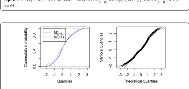
Figure 1A comparison fitted distribution functions ofM_βnˆ–β

0andN(0, 1), and QQ-plot ofMβnˆ–β0, where

n= 64

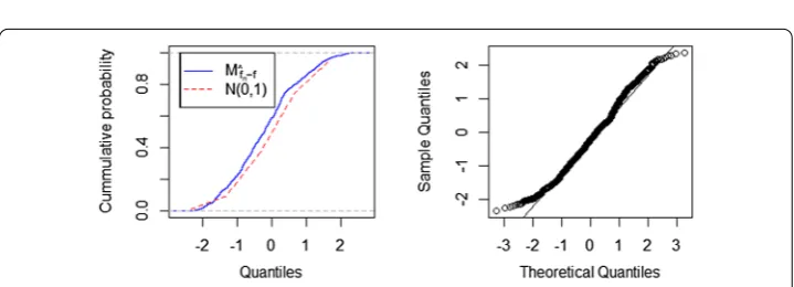
Figure 2A comparison fitted distribution functions ofM_βnˆ–β

0andN(0, 1), and QQ-plot ofMβnˆ–β0, where

n= 128

Setm= 3 and the difference sequenced0=√3/4,d1=d2=d3= –√1/12 (Wang et al. [9]). We first evaluate theMβˆn–β0= (n–m)

–1_2τ–1

β n(βˆn–β0) approximation. Figures1and

2show the results for two sample size specifications (n= 64,n= 128). Panel 1 in Fig.1 com-pares the empirical distribution functions ofMβˆn–β0andN(0, 1). Panel 2 in Fig.1gives the QQ-plot ofMβˆn–β0. Figure1shows that the distribution ofMβˆn–β0can approximateN(0, 1) well even if the sample size are not large (n= 64). Comparison of Fig.2with Fig.1indicates that the distribution approximation for the larger sample size is much more accurate than that for the small one.

Choose the Daubechies scaling function2φ(t) as in Hu et al. [29]. Figures3and4show

that the distribution of Mˆfn–f =τt–1(ˆfn(t) –f(t)) is closer and closer to N(0, 1) with the

increasing sample size.

6 Conclusions

Figure 3A comparison fitted distribution functions ofM_ˆ

fn–fandN(0, 1), and QQ-plot ofMˆfn–f, wheren= 64

Figure 4A comparison fitted distribution functions ofM_ˆ

fn–fandN(0, 1), and QQ-plot ofMˆfn–f, wheren= 128

Funding

The research is supported by National Natural Science Foundation of China [grant number 71471075].

Competing interests

The authors declare that they have no competing interests.

Authors’ contributions

All authors contributed equally to the writing of this paper. All authors read and approved the final manuscript.

Publisher’s Note

Springer Nature remains neutral with regard to jurisdictional claims in published maps and institutional affiliations.

Received: 10 June 2018 Accepted: 18 September 2018

References

1. Engle, R.F., Granger, C.W.J., Rice, J., Weiss, A.: Semiparametric estimates of the relation between weather and electricity sales. J. Am. Stat. Assoc.81, 310–320 (1986)

2. Silvapullé, M.J.: Asymptotic behavior of robust estimators of regression and scale parameters with fixed carriers. Ann. Stat.13(4), 1490–1497 (1985)

3. Kim, S., Cho, H.R.: Efficient estimation in the partially linear quantile regression model for longitudinal data. Electron. J. Stat.12(1), 824–850 (2018)

4. Härdle, W., Gao, J., Liang, H.: Partially Linear Models. Springer, New York (2000)

5. Chang, X.W., Qu, L.: Wavelet estimation of partially linear models. Comput. Stat. Data Anal.47, 31–48 (2004) 6. Liang, H., Wang, S.J., Carroll, R.J.: Partially linear models with missing response variables and error-prone covariates.

Biometrika94(1), 185–198 (2007)

7. Holland, A.D.: Penalized spline estimation in the partially linear model. J. Multivar. Anal.153, 211–235 (2017) 8. Zhao, T., Cheng, G., Liu, H.: A partially linear framework for massive heterogeneous data. Ann. Stat.44(4), 1400–1437

(2016)

9. Wang, L., Brown, L.D., Cai, T.T.: A difference based approach to the semiparametric partial linear model. Electron. J. Stat.5, 619–641 (2011)

10. Tabakan, G., Akdeniz, F.: Difference-based ridge estimator of parameters in partial linear model. Stat. Pap.51, 357–368 (2010)

11. Duran, E.A., Hädle, W.K., Osipenko, M.: Difference based ridge and Liu type estimators in semiparametric regression models. J. Multivar. Anal.105(1), 164–175 (2012)

13. Wu, J.: Restricted difference-based Liu estimator in partially linear model. J. Comput. Appl. Math.300, 97–102 (2016) 14. Shen, Y., Wang, X.J., Yang, W.Z., Hu, S.H.: Almost sure convergence theorem and strong stability for weighted sums of

NSD random variables. Acta Math. Sin. Engl. Ser.29(4), 743–756 (2013)

15. Xue, Z., Zhang, L.L., Lei, Y.J., Chen, Z.J.: Complete moment convergence for weighted sums of negatively superadditive dependent random variables. J. Inequal. Appl.2015, Article ID 117 (2015)

16. Shen, Y., Wang, X.J., Hu, S.H.: On the strong convergence and some inequalities for negatively superadditive dependent sequences. J. Inequal. Appl.2013, Article ID 448 (2013)

17. Wang, X.J., Deng, X., Zheng, L.L., Hu, S.H.: Complete convergence for arrays of rowwise negatively superadditive dependent random variables and its applications. Statistics48(4), 834–850 (2014)

18. Wang, X.J., Shen, A.T., Chen, Z.Y., Hu, S.H.: Complete convergence for weighted sums of NSD random variables and its application in the EV regression model. Test24, 166–184 (2015)

19. Meng, B., Wang, D., Wu, Q.: On the strong convergence for weighted sums of negatively superadditive dependent random variables. J. Inequal. Appl.2017, Article ID 269 (2017)

20. Shen, A.T., Wang, X.H.: Kaplan–Meier estimator and hazard estimator for censored negatively superadditive dependent data. Statistics50(2), 377–388 (2016)

21. Shen, A.T., Xue, M.X., Volodin, A.: Complete moment convergence for arrays of rowwise NSD random variables. Stochastics88(4), 606–621 (2016)

22. Wang, X.J., Wu, Y., Hu, S.H.: Strong and weak consistency of LS estimators in the EV regression model with negatively superadditive-dependent errors. AStA Adv. Stat. Anal.102, 41–65 (2018)

23. Wang, X.J., Wu, Y., Hu, S.H.: Complete moment convergence for double-indexed randomly weighted sums and its applications. Statistics52(3), 503–518 (2018)

24. Kemperman, J.H.B.: On the FKG-inequalities for measures on a partially ordered space. Proc. Akad. Wet., Ser. A80, 313–331 (1977)

25. Hu, T.Z.: Negatively superadditive dependence of random variables with applications. Chinese J. Appl. Probab. Statist.

16(2), 133–144 (2000)

26. Gannaz, I.: Robust estimation and wavelet thresholding in partially linear models. Stat. Comput.17, 293–310 (2007) 27. Hu, H.C., Wu, L.: Convergence rates of wavelet estimators in semiparametric regression models under NA samples.

Chin. Ann. Math.33(4), 609–624 (2012)

28. Christophe, C., Isha, D., Hassan, D.: Nonparametric estimation of a quantile density function by wavelet methods. Comput. Stat. Data Anal.94, 161–174 (2016)

29. Hu, H.C., Cui, H.J., Li, K.C.: Asymptotic properties of wavelet estimators in partially linear errors-in-variables models with long memory errors. Acta Math. Appl. Sin. Engl. Ser.34(1), 77–96 (2018)

30. Yatchew, A.: An elementary estimator for the partial linear model. Econ. Lett.5, 135–143 (1997)

31. Zhao, H., You, J.: Difference based estimation for partially linear regression models with measurement errors. J. Multivar. Anal.102, 1321–1338 (2011)

32. Lehmann, E.L.: Some concepts of dependence. Ann. Math. Stat.37, 1137–1153 (1966) 33. Rao, B.L.S.P.: Asymptotic Theory of Statistical Inference. Wiley, New York (1987)