Comparing the excepted values of atom bond connectivity and geometric–arithmetic indices in random spiro chains

R E S E A R C H

Open Access

Comparing the excepted values of

atom-bond connectivity and

geometric–arithmetic indices in random

spiro chains

Shouliu Wei

_{, Xiaoling Ke}

_{and Guoliang Hao}

*_{Correspondence:}

[email protected] 1_{Department of Mathematics,}

Minjiang University, Fuzhou, P.R. China

Full list of author information is available at the end of the article

Abstract

The atom-bond connectivity (ABC) index and geometric–arithmetic (GA) index are two well-studied topological indices, which are useful tools in QSPR and QSAR investigations. In this paper, we first obtain explicit formulae for the expected values ofABCandGAindices in random spiro chains, which are graphs of a class of unbranched polycyclic aromatic hydrocarbons. Based on these formulae, we then present the average values ofABCandGAindices with respect to the set of all spiro chains withnhexagons and make a comparison between the expected values ofABC andGAindices in random spiro chains.

MSC: 05C05; 05C12

Keywords: ABCindex;GAindex; Spiro chain; Average value; Comparison

1 Introduction

A connected graph with maximum vertex degree at most 4 is said to be amolecular graph. Its graphical representation may resemble a structural formula of some (usually organic) molecule. That was a primary reason for employing graph theory in chemistry. Nowa-days this area of mathematical chemistry is calledchemical graph theory[1]. Molecular descriptors play a significant role and have found wide applications in chemical graph the-ory especially in investigations of the quantitative structure-property relations (QSPR) and quantitative structure-activity relations (QSAR). Among them, topological indices have a prominent place [2]. There exists a legion of topological indices that have some applica-tions in chemistry [2, 3]. One of the best known and widely used topological indices is the connectivity index (Randić index) introduced in 1975 by Randić [4], who has shown that this index can reflect molecular branching. Some results on molecular branching can be found in [5–9] and the references therein. However, many physico-chemical properties depend on factors rather different from branching.

All graphs considered in this paper are simple, undirected, and connected. The notation not defined in this paper can be found in the book [10]. LetGbe a graph with vertex set

V(G) ={v1,v2, . . . ,vn}and edge setE(G). Denote bydithe degree of the vertexviinG. If an

edge connects a vertex of degreeiand a vertex of degreejinG, then we call it an (i,j)-edge. Letmij(G) denote the number of (i,j)-edges inG.

In 1998, Estrada et al. [11] proposed a topological index of a graphG, known as the

atom-bond connectivity index, which is abbreviated asABC(G) and defined as

ABC(G) =

vivj∈E(G)

di+dj– 2

didj

, (1)

where the summation goes over all edges ofG. TheABCindex has been proven to be a valuable predictive index in the study of the heat of formation in alkanes and has been applied up to now to study the stability of alkanes and the strain energy of cycloalkanes [11, 12]. For some recent contributions on theABCindex, we refer to [13–17].

As an analogue to theABCindex, a new topological index of a graphG, named the

geometric–arithmetic indexand abbreviatedGA(G), was considered by Vukićević and Fur-tula [18] in 2009. TheGAindex is defined as follows:

GA(G) =

vivj∈E(G)

2didj

di+dj

, (2)

where the summation goes over all edges ofG. It is noted in [18] that theGAindex is well correlated with a variety of physico-chemical properties and the predictive power ofGA

index is somewhat better than the Randić index. Up to now, many mathematical properties ofGAindex were investigated in [15, 19–23] and the references therein.

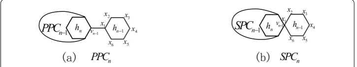
Polyphenyls and their derivatives, which can be used in organic synthesis, drug synthe-sis, heat exchanger, and so on, attracted the attention of chemists for many years [24–26]. Apolyphenyl chainof lengthnis obtained from a sequence of hexagonsh1,h2, . . . ,hnby

adding a cut edge to each pair of consecutive hexagons, which is denoted byPPCn. The

hexagonhi is called theith hexagonofPPCnfor 1≤i≤n. Figure 1(a) shows a general

polyphenyl chain, wherevn–1is a vertex ofhn–1inPPCn–1. Note that, there are three ways

to add a cut edge between two consecutive hexagons. SoPPCnis not unique whenn≥3.

Lethn–1=x1x2x3x4x5x6inPPCn–1forn≥3. There is a cut edge connectingx1andvn–2,

which is a vertex inhn–2. By symmetry there are three ways to add a cut edge between the

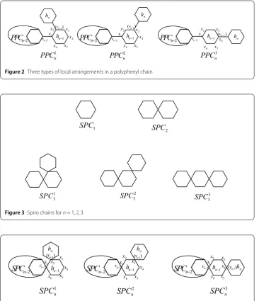
(n– 1)th hexagonhn–1ofPPCn–1to the extra hexagonhn. Precisely, letPPC1n,PPC2n, and

PPC3

nbe the graphs obtained by adding a cut edge connecting a vertex of the extra hexagon

hnwith vertexxi+1ofhn–1(see Figure 2), wherei= 1, 2, 3. Many results on matching and

independent set, Wiener index, Merrified–Simmons index, Kirchhoff index, and Hosoya index of polyphenyl chains were reported in [27–32] and the references therein.

Figure 2Three types of local arrangements in a polyphenyl chain

Figure 3Spiro chains forn= 1, 2, 3

Figure 4Three types of local arrangements in the spiro chain corresponding to a polyphenyl chain

A spiro chain of lengthn, denotedSPCn, can be obtained from a polyphenyl chainPPCn

by contracting each cut edge between each pair of consecutive hexagons inPPCn. Figure 3

shows the unique spiro chains forn= 1, 2 and all spiro chains forn= 3, and Figure 1(b) shows a general case, wherevn–1is a vertex ofhn–1inSPCn–1. Similarly to the construction

of a polyphenyl chainPPCn, it is clear thatSPCnis also not unique whenn≥3 and has

three types of local arrangements, which are denoted bySPC1_n,SPC2_n, andSPC3_n(Figure 4). We may assume that getting anSPCnfrom a fixedSPCn–1is a random process. Namely,

the probabilities of gettingSPC1

n, SPC2n, and SPC3nfrom a fixedSPCn–1 arep1,p2, and

1 –p1–p2, respectively. We also assume that the probabilitiesp1andp2are constants and independent ofn, that is, the process described is a zeroth-order Markov process. After associating probabilities, such a spiro chain is called arandom spiro chainand denoted by

SPC(n;p1,p2). For some contributions on spiro chains, the readers are referred to [27, 28,

in a random spiro chain. For more results concerning other random chains, we refer to [36–42] and the references therein.

The rest of this paper is organized as follows. In Section 2, we present explicit formulae for the expected values of theABCandGAindices of random spiro chains. Based on these formulae, we then give the average values of theABCandGAindices with respect to the set of all spiro chains withnhexagons in Section 3 and make a comparison between the expected values of theABCandGAindices in random spiro chains in Section 4.

2 TheABCandGAindices in random spiro chains

In this section, we consider theABCandGAindices in a random spiro chain. We keep the notation defined in Section 1. LetSPCnbe the spiro chain obtained by attaching a

new hexagonhntoSPCn–1as described in Figure 1(b). Assume thathn=x1x2x3x4x5x6as

shown in Figure 2. Clearly, there are only (2, 2)-, (2, 4)-, and (4, 4)-edges in a spiro chain

SPCn. By the definitions of theABCandGAindices we can directly check that

ABC(SPCn) =

√

2

2 m22(SPCn) +

√

2

2 m24(SPCn) +

√

6

4 m44(SPCn) (3) and

GA(SPCn) =m22(SPCn) +

2√2

3 m24(SPCn) +m44(SPCn). (4) Thus, to compute theABCandGAindices ofSPCn, we just need to determinem22(SPCn),

m24(SPCn), andm44(SPCn).

Recall thatSPC(n;p1,p2) is a random spiro chain of lengthn. Clearly, bothABC(SPC(n; p1,p2)) andGA(SPC(n;p1,p2)) are random variables. For convenience, denote their ex-pected values byEa

n=E[ABC(SPC(n;p1,p2))] andE g

n=E[GA(SPC(n;p1,p2))], respectively.

We first give a formula for the expected value of theABCindex of a random spiro chain.

Theorem 2.1 Let SPC(n;p1,p2)be a random spiro chain of length n≥1.Then

EABCSPC(n;p1,p2)=

√

6 4 –

√

2 2

p1+ 3√2

n+

√

2 2 –

√

6 4

p1.

Proof Whenn= 1, there is only one hexagon. SoEa

1= 6×

√

2 2 = 3

√

2.

Whenn≥2, it is obvious thatm22(SPCn),m24(SPCn), andm44(SPCn) depend on the

three possible constructions as shown in Figure 3. (i) IfSPCn–1→SPC1nwith probabilityp1, then we have

m22SPC1_n=m22(SPCn–1) + 3,m24

SPC1_n=m24(SPCn–1) + 2

and

m44

SPC1_n=m44(SPCn–1) + 1.

Therefore by (3) we have

ABCSPC1_n=ABC(SPCn–1) +

5√2 2 +

√

(ii) IfSPCn–1→SPC2nwith probabilityp2, then we have

m22SPC2_n=m22(SPCn–1) + 2,m24

SPC2_n=m24(SPCn–1) + 4

and

m44SPC2_n=m44(SPCn–1).

Therefore by (3) we have

ABCSPC2_n=ABC(SPCn–1) + 3 √

2.

(iii) IfSPCn–1→SPC3nwith probability 1 –p1–p2, then we have m22SPC3_n=m22(SPCn–1) + 2,m24

SPC3_n=m24(SPCn–1) + 4

and

m44SPC3_n=m44(SPCn–1).

Therefore by (3) we have

ABCSPC3_n=ABC(SPCn–1) + 3 √

2. Thus we obtain

Ea_n=EABCSPC(n,p1,p2) =p1ABC

SPC1_n+p2ABC

SPC2_n+ (1 –p1–p2)ABC

SPC3_n

=ABC(SPCn–1) + √

6 4 –

√

2 2

p1+ 3√2.

Note thatE[Ea

n] =Ena. Applying the expectation operator to the last equation, we get

Ea_n=E_na_–1+

√

6 4 –

√

2 2

p1+ 3

√

2 forn≥2. (5)

Since equation (5) is a first-order nonhomogeneous linear difference equation with con-stant coefficients. It is clear that the general solution of the homogeneous part of equation (5) isEa_{=c, a constant.}

LetEa∗_{=anbe a particular solution of equation (5). SubstitutingE}a∗_{into equation (5)}

and comparing the constant term, we have

a=

√

6 4 –

√

2 2

p1+ 3√2.

Consequently, the general solution of equation (5) is

Ea_n=Ea∗+Ea=EABCSPC(n;p1,p2)

=

√

6 4 –

√

2 2

p1+ 3

√

2

Substituting the initial condition, we obtain

C=

√

2 2 –

√

6 4

p1.

Therefore we have

Ea_n=

√

6 4 –

√

2 2

p1+ 3√2

n+

√

2 2 –

√

6 4

p1.

This completes the proof. We now give the formula for the expected value of theGAindex of a random spiro chain.

Theorem 2.2 Let SPC(n;p1,p2)be a random spiro chain of length n≥1.Then

EGASPC(n;p1,p2)

= 2 –4

√

2 3

p1+ 2 +

8√2 3

n+

4√2 3 – 2

p1+

4 –8

√

2 3

.

Proof Whenn= 1, there is only one hexagon. SoEg₁=E[GA(SPC(1;p1,p2))] = 6.

Whenn≥2, it is obvious thatm22(SPCn),m24(SPCn), andm44(SPCn) depend on the

three possible constructions as shown in Figure 3. (i) IfSPCn–1→SPC1nwith probabilityp1, then we get

m22

SPC1_n=m22(SPCn–1) + 3,m24

SPC1_n=m24(SPCn–1) + 2

and

m44

SPC1_n=m44(SPCn–1) + 1.

Therefore by (4) we have

GASPC1_n=GA(SPCn–1) + 4 +

4√2 3 .

(ii) IfSPCn–1→SPC2nwith probabilityp2, then we get

m22

SPC2_n=m22(SPCn–1) + 2,m24

SPC2_n=m24(SPCn–1) + 4

and

m44

SPC2_n=m44(SPCn–1).

Therefore by (4) we have

GASPC2_n=GA(SPCn–1) + 2 +

(iii) IfSPCn–1→SPC3nwith probability 1 –p1–p2, then we have

m22SPC3_n=m22(SPCn–1) + 2,m24

SPC3_n=m24(SPCn–1) + 4

and

m44SPC3_n=m44(SPCn–1).

Therefore by (4) we have

GASPC3_n=GA(SPCn–1) + 2 +

8√2 3 . Thus we obtain

Eg_n=EGASPC(n,p1,p2) =p1GA

SPC1_n+p2GA

SPC2_n+ (1 –p1–p2)GA

SPC3_n

=GA(SPCn–1) +

2 –4

√ 2 3 p1+

2 +8

√

2 3

.

Note thatE[Egn] =Egn. Applying the expectation operator to the last equation, we get

Eg_n=Eg_n–1+

2 –4

√ 2 3 p1+

2 +8

√

2 3

, forn≥2. (6)

Since equation (6) is a first-order nonhomogeneous linear difference equation with con-stant coefficients, it is clear that the general solution of the homogeneous part of equation (6) isEg_{=c, a constant.}

LetEg∗_{=anbe a particular solution of equation (6). SubstitutingE}g∗_{into equation (6)}

and comparing the constant term, we have

a=

2 –4

√

2 3

p1+

2 +8

√

2 3

.

Consequently, the general solution of equation (6) is

Eg_n=Eg∗+Eg=EGASPC(n;p1,p2)

= 2 –4

√ 2 3 p1+

2 +8

√

2 3

n+C forn≥1.

Substituting the initial condition, we obtain

C=

4√2 3 – 2

p1+

4 –8

√

2 3

.

Therefore we have

Eg_n= 2 –4

√ 2 3 p1+

2 +8

√ 2 3 n+

4√2 3 – 2

p1+

4 –8

√

2 3

,

In Theorems 2.1 and 2.2, we observe that bothE[ABC(SPC(n;p1,p2))] andE[GA(SPC(n;

p1,p2))] are asymptotic tonand linear inp1. Therefore, by Theorems 2.1 and 2.2 we can easily obtain theABCandGAindices of spiro meta-chainOn, spiro orth-chainMn, and

spiro para-chainPn(defined in [30]).

Corollary 2.3 The ABC indices of the spiro meta-chain On,the spiro orth-chain Mn,and

the spiro para-chain Pnare

ABC(On) =

√

6 4 +

5√2 2

n+

√

2 2 –

√

6 4

and

ABC(Mn) =ABC(Pn) = 3

√

2n.

Corollary 2.4 The GA indices of the spiro meta-chain On,the spiro orth-chain Mn,and

the spiro para-chain Pnare

GA(On) =

4 +4

√

2 3

n+ 2 –4

√

2 3

and

GA(Mn) =GA(Pn) =

2 +8

√

2 3

n+ 4 –8

√

2 3 .

3 The average values ofABCandGAindices

In this section, we present the average values of theABCandGAindices with respect to the set of all spiro chains withnhexagons.

LetSPnbe the set of all spiro chains withnhexagons. The average values of theABC

andGAindices ofSPnare defined by

ABCavr(SPn) =

1

|SPn|

G∈SPn

ABC(G)

and

GAavr(SPn) =

1

|SPn|

G∈SPn GA(G),

respectively. In fact, this is the population mean of theABCandGAindices of all elements inSPn. Since every element occurring inSPnhas the same probability, we havep1=p2=

1 –p1–p2. Thus we can apply Theorems 2.1 and 2.2 by puttingp1=p2= 1 –p1–p2=1₃ and obtain the following result.

Theorem 3.1 The average values of the ABC and GA indices with respect toSPnare

ABCavr(SPn) =

√

6 12 +

17√2 6

n+

√

2 6 –

√

and

GAavr(SPn) =

8 3+

20√2 9

n+10

3 – 20√2

9 .

From Theorem 3.1, as well as from Corollaries 2.3 and 2.4, it is no difficult to see that the average values of theABCandGAindices with respect to{On,Mn,Pn}are

ABC(On) +ABC(Mn) +ABC(Pn)

3 =

√

6 12 +

17√2 6

n+

√

2 6 –

√

6 12 and

GA(On) +GA(Mn) +GA(Pn)

3 =

8 3+

20√2 9

n+10

3 – 20√2

9 ,

which indicate that the average values of theABCandGAindices with respect toSPnare

exactly equal to the average values of theABCandGAindices with respect to{On,Mn,Pn},

respectively.

4 A comparison between the expected values ofABCandGAindices

Das and Trinajstić [15] compared the firstGAindex andABCindex for chemical trees, molecular graphs, and simple graphs with some restricted conditions. Recently, Ke [40] also compared the expected values of the GAindex and ABCindex for a random polyphenyl chain. Using Theorems 2.1 and 2.2, we now make a comparison between the expected values for theABCandGAindices of a random spiro chain with the same prob-abilitypi(i= 1, 2).

Theorem 4.1 Let SPC(n;p1,p2)be a random spiro chain with n hexagons.Then

EGA(SPC(n;p1,p2)>EABC(SPC(n;p1,p2).

Proof Whenn= 1, it is clear that

EGA(SPC(1;p1,p2)= 6 > 3√2 =EABC(SPC(1;p1,p2).

Whenn≥2, by Theorems 2.1 and 2.2 we have

EGA(SPC(n;p1,p2)–EABC(SPC(n;p1,p2) = 2 –

√

6 4 –

4√2 3 +

√

2 2

p1+ 2 +8

√

2 3 – 3

√

2

n

+

4√2 3 – 2 –

√

2 2 +

√

6 4

p1+ 4 –8

√

Noting that 2 –

√

6 4 –

4√2 3 +

√

2

2 > 0 and 0≤p1≤1, we get EGA(SPC(n;p1,p2)

–EABC(SPC(n;p1,p2)

≥

2 +8

√

2 3 – 3

√

2

n+

4√2 3 – 2 –

√

2 2 +

√

6 4

×1 + 4 –8

√

2 3 =

2 –

√

2 3

n+ 2 +

√

6 4 –

11√2 6

≥

2 –

√

2 3

×2 + 2 +

√

6 4 –

11√2 6 > 0,

as desired. This completes the proof. Theorem 4.1 states that the expected value of theABCindex is less than the expected value of theGAindex for a random spiro chain, which is similar to the result for a random polyphenyl chain [40].

5 Conclusions

In this paper, we mainly study theABCandGAindices in random spiro chains. Firstly, we study explicit formulae for the expected values of theABCandGAindices in random spiro chains, similar to the results obtained in [30, 33]. Secondly, we present the average values of theABCandGAindices with respect to the set of all spiro chains withnhexagons. Finally, we compare the expected values of theABCandGAindices in random spiro chains and show that the expected value of theABCindex is less than the expected value of theGA

index.

Acknowledgements

The authors would like to thank the anonymous referees for their constructive suggestions and valuable comments on this paper, which have contributed to the final preparation of the paper. This project is supported by Natural Science Foundation of Fujian Province under Grant No. 2015J01589, Science Foundation for the Education Department of Fujian Province under Grant No. JAT160386, and Science Foundation of Minjiang University under Grants Nos. MYK15004, Mjyp201608.

Competing interests

The authors declare that they have no competing interests.

Authors’ contributions

SW carried out the proofs of the main results in the manuscript. XK and GH participated in the design of the study and drafted the manuscript. All the authors read and approved the final manuscript.

Author details

1_{Department of Mathematics, Minjiang University, Fuzhou, P.R. China.}2_{College of Science, East China University of}

Technology, Nanchang, P.R. China.

Publisher’s Note

Springer Nature remains neutral with regard to jurisdictional claims in published maps and institutional affiliations.

Received: 29 July 2017 Accepted: 7 February 2018

References

1. Trinajsti´c, N.: Chemical Graph Theory. CRC Press, Boca Raton (1983)

5. Gutman, I., Vukiˇcevi´c, D., Žerovnik, J.: A class of modified Wiener indices. Croat. Chem. Acta77, 103–109 (2004) 6. Vukiˇcevi´c, D.: Distinction between modifications of Wiener indices. MATCH Commun. Math. Comput. Chem.47,

87–105 (2003)

7. Vukiˇcevi´c, D., Gutman, I.: Note on a class of modified Wiener indices. MATCH Commun. Math. Comput. Chem.47, 107–117 (2003)

8. Vukiˇcevi´c, D., Žerovnik, J.: Variable Wiener indices. MATCH Commun. Math. Comput. Chem.53, 385–402 (2005) 9. Vukiˇcevi´c, D., Žerovnik, J.: New indices based on the modified Wiener indices. MATCH Commun. Math. Comput.

Chem.60, 119–132 (2008)

10. Bondy, J.A., Murty, U.S.R.: Graph Theory with Applications. MacMillan, New York (1976)

11. Estrada, E., Torres, L., Rodríguez, L., Gutman, I.: An atom-bond connectivity index: modelling the enthalpy of formation of alkanes. Indian J. Chem.37A, 849–855 (1998)

12. Estrada, E.: Atom-bond connectivity and the energetic of branched alkanes. Chem. Phys. Lett.463, 422–425 (2008) 13. Chen, J., Guo, X.: Extreme atom-bond connectivity index of graphs. MATCH Commun. Math. Comput. Chem.65,

713–722 (2011)

14. Das, K.C.: Atom-bond connectivity index of graphs. Discrete Appl. Math.158, 1181–1188 (2010)

15. Das, K.C., Trinajsti´c, N.: Comparison between first geometric–arithmetic index and atom-bond connectivity index. Chem. Phys. Lett.497, 149–151 (2010)

16. Ke, X.: Atom-bond connectivity index of benzenoid systems and fluoranthene congeners. Polycycl. Aromat. Compd.

32, 27–35 (2012)

17. Furtula, B., Graovac, A., Vukiˇcevi´c, D.: Atom-bond connectivity index of trees. Discrete Appl. Math.157, 2828–2835 (2009)

18. Vukiˇcevi´c, D., Furtula, B.: Topological index based on the ratios of geometrical and arithmetical means of end-vertex degrees of edges. J. Math. Chem.46, 1369–1376 (2009)

19. Das, K.C.: On geometric–arithmetic index of graphs. MATCH Commun. Math. Comput. Chem.64(3), 619–630 (2010) 20. Divni´c, T., Milivojevi´c, M., Pavlovi´c, L.: Extremal graphs for the geometric–arithmetic index with given minimum

degree. Discrete Appl. Math.162, 386–390 (2014)

21. Rodríguez, J.M., Sigarreta, J.M.: Spectral properties of geometric–arithmetic index. Appl. Math. Comput.277, 142–153 (2016)

22. Yuan, Y., Zhou, B., Trinajsti´c, N.: On geometric–arithmetic index. J. Math. Chem.47, 833–841 (2010)

23. Zhou, B., Gutman, I., Furtula, B., Du, Z.: On two types of geometric–arithmetic index. Chem. Phys. Lett.482, 153–155 (2009)

24. Flower, D.R.: On the properties of bit string-based measures of chemical similarity. J. Chem. Inf. Comput. Sci.38, 379–386 (1998)

25. Li, Q.R., Yang, Q., Yin, H., Yang, S.: Analysis of by-products from improved Ullmann reaction using TOFMS and GCTOFMS. J. Univ. Sci. Technol. China34, 335–341 (2004)

26. Tepavcevic, S., Wroble, A.T., Bissen, M., Wallace, D.J., Choi, Y., Hanley, L.: Photoemission studies of polythiophene and polyphenyl films produced via surface polymerization by ion-assisted deposition. J. Phys. Chem. B109, 7134–7140 (2005)

27. Deng, H.: Wiener indices of spiro and polyphenyl hexagonal chains. Math. Comput. Model.55, 634–644 (2012) 28. Deng, H., Tang, Z.: Kirchhoff indices of spiro and polyphenyl hexagonal chains. Util. Math.95, 113–128 (2014) 29. Došli´c, T., Litz, M.S.: Matchings and independent sets in polyphenylene chains. MATCH Commun. Math. Comput.

Chem.67, 313–330 (2012)

30. Huang, G., Kuang, M., Deng, H.: The expected values of Kirchhoff indices in the random polyphenyl and spiro chains. Ars Math. Contemp.9, 197–207 (2015)

31. Huang, G., Kuang, M., Deng, H.: The expected values of Hosoya index and Merrifield–Simmons index in a random polyphenylene chain. J. Comb. Optim.32, 550–562 (2016)

32. Yang, W., Zhang, F.: Wiener index in random polyphenyl chains. MATCH Commun. Math. Comput. Chem.68, 371–376 (2012)

33. Chen, X., Zhao, B., Zhao, P.: Six-membered ring spiro chains with extremal Merrifild–Simmons index and Hosaya index. MATCH Commun. Math. Comput. Chem.62, 657–665 (2009)

34. Yang, Y., Liu, H., Wang, H., Fu, H.: Subtrees of spiro and polyphenyl hexagonal chains. Appl. Math. Comput.268, 547–560 (2015)

35. Yang, Y., Liu, H., Wang, H., Sun, S.: On spiro and polyphenyl hexagonal chains with respect to the number of BC-subtrees. Int. J. Comput. Math.94(4), 774–799 (2017)

36. Chen, A., Zhang, F.: Wiener index and perfect matchings in random phenylene chains. MATCH Commun. Math. Comput. Chem.61, 623–630 (2009)

37. Gutman, I., Kennedy, J.W., Quintas, L.V.: Wiener numbers of random benzenoid chains. Chem. Phys. Lett.173, 403–408 (1990)

38. Gutman, I.: The number of perfect matchings in a random hexagonal chain. Graph Theory Notes N. Y.16, 26–28 (1989)

39. Gutman, I., Kennedy, J.W., Quintas, L.V.: Perfect matchings in random hexagonal chain graphs. J. Math. Chem.6, 377–383 (1991)