R E S E A R C H
Open Access
M-test in linear models with negatively
superadditive dependent errors
Yuncai Yu
1*, Hongchang Hu
2, Ling Liu
3and Shouyou Huang
2*Correspondence:
1State Key Laboratory of Mechanics
and Control of Mechanical Structures, Institute of Nano Science and Department of Mathematics, Nanjing University of Aeronautics and Astronautics, Nanjing, 210016, China
Full list of author information is available at the end of the article
Abstract
This paper is concerned with the testing hypotheses of regression parameters in linear models in which errors are negatively superadditive dependent (NSD). A robust M-test base on M-criterion is proposed. The asymptotic distribution of the test statistic is obtained and the consistent estimates of the redundancy parameters involved in the asymptotic distribution are established. Finally, some Monte Carlo simulations are given to substantiate the stability of the parameter estimates and the power of the test, for various choices of M-methods, explanatory variables and different sample sizes.
MSC: 60F05; 60G10; 62F35; 62M10; 60G42
Keywords: NSD random sequences; linear regression models; M-test; asymptotic property; Monte Carlo simulations
1 Introduction
Consider the linear regression model:
yt= xtβ+et, t= , . . . ,n, ()
where{yt}and{xt= (xt,xt, . . . ,xtp)}are real-valued responses and real-valued random
vectors, respectively. The superscriptrepresents the transpose throughout this paper, β= (β, . . . ,βp)is ap-vector of the unknown parameter, and{et}are random errors.
It is well known that linear regression models have received much attentions for their immense applications in various areas such as engineering technology, economics and social sciences. Unfortunately, there exists the problem that the classical maximum like-lihood estimator for these models is sufficiently sensitive to outliers. To overcome this defect, Huber proposed the M-estimate which possesses the robustness (see Huber []) by minimizing
n
t=
ρyt– xt β, ()
whereρ is a convex function. It is obvious that many important estimates can be ad-dressed easily. For instance, the least square (LS) estimate withρ(x) =x/, the least
absolute deviation (LAD) estimate withρ(x) =|x|, and the Huber estimate withρ(x) = (xI(|x| ≤k))/ + (k|x|–k/)I(|x|>k),k> , whereI(A)is the indicator function ofA.
Letβˆnbe a minimizer of () and consequentlyβˆnis a M-estimate ofβ. Some excellent results as regards the asymptotic properties ofβnˆ with various forms ofρhave been re-ported in [–]. Most of the results rely on the independence errors. As Huber claimed in [], the independence assumption on the errors is a serious restriction. It is practically essential and imperative to explore the case of dependent errors, which is a theoretically challenging. Under the dependence assumption of the errors, Berlinetet al.[] proved the consistency of M-estimates for linear models with strong mixing errors. Cuiet al.[] obtained the asymptotic distributions of M-estimates for linear models with spatially cor-related errors. Wu [] investigated the weak and strong Bahadur representations of the M-estimates for linear models with stationary causal errors. Wu [] established the strong consistency of M-estimates for linear models with negatively dependent (NA) random er-rors.
In the following we will introduce a wide random sequence, NSD random sequence, whose definition based on the superadditive functions.
Definition (Hu []) A functionφ:Rn→R, is called superadditive if
φ(x∨y) +φ(x∧y)≥φ(x) +φ(y),
for all x, y∈Rn, where ‘∨’ is for a componentwise maximum and ‘∧’ is for a component-wise minimum.
Definition (Hu []) A random vector (X,X, . . . ,Xn) is said to be NSD if
Eφ(X,X, . . . ,Xn)≤Eφ
X∗,X∗, . . . ,Xn∗, ()
where{Xt∗,t= , . . . ,n}are independent random variables such that have same marginal distribution with{Xt,t= , . . . ,n}for eacht, andφ is a superadditive function such that the expectations in () exist.
Definition (Wanget al.[]) A sequence of random variables (X, . . . ,Xn) is called NSD
if for alln≥, (X, . . . ,Xn) is NSD.
The purpose of this paper is to investigate the M-test problem of the regression pa-rameters in the model () with NSD random errors, we consider a test for the following hypothesis:
H: H(β– b) = versus H: H(β– b)= , ()
where H is a knownp×qmatrix with the rankq( <q≤p), b is a knownp-vector. A sequence of the local alternatives is considered as follows:
H,n: H(β– b) = Hωn, ()
whereωnis a knownp-vector such that
S/n ωn=O(), ()
where Sn=nt=xtxTt,·is the Euclidean norm. Denote
min
H(β–b)=
n
t=
ρyt– xt β= n
t=
ρyt– xtβ˜,
min
β∈Rp
n
t=
ρyt– xt β= n
t=
ρyt– xt βˆ,
Mn= n
t=
ρyt– xtβ˜– n
t=
ρyt– xt βˆ.
Actually,β˜andβˆare the M-estimates in the restricted and unrestricted model (), respec-tively. To test the hypothesis (), we adopt M-criterion which regardsMnas the criterion to measure the level of departure from the null hypothesis. Several classical conclusions have been presented in [–] when the errors are assumed to be independence, we will generalize the case to NSD random errors. Throughout this paper, letCbe a positive constant. Put|τ|=max≤t≤p{|τ|,|τ|, . . . ,|τp|}ifτ is ap-vector. Letx+=xI(x≥) and x–= –xI(x< ). A random sequence{Xn}is said to onLq-norm,q> , ifE|Xn|q<∞. De-notean=oP(bn) ifan/bnconverges to in probability andan=OP(bn) ifan/bnconverges to a constant in probability.
The rest of the paper is organized as follows. In Section , the asymptotic distribution of Mnis obtained with the NSD random errors, and the consistence estimates of the redun-dancy parametersλandσ are constructed under the local hypothesis. Section gives
the theoretical proofs of main results. The simulations are presented to show the per-formances of parameter estimates and the M-test for the powers in Section , and the conclusions are given in Section .
2 Main results
In this paper, letρbe a non-monotonic convex function onR, and denoteψ+andψ–as
the right and left derivatives of the functionρ, respectively. The derivative functionψis chosen to satisfyψ–(u)≤ψ(u)≤ψ+(u), for allu∈R.
(A) The functionG(u) =Eψ(et+u)exists withG() =Eψ(et) = , and has a positive derivativeλatu= .
(A) <Eψ(e) =σ<∞, andlimu→E|ψ(e+u) –ψ(e)|= .
(A) There exists a positive constantsuch that forh∈(,), the function ψ(u+h) –ψ(u)is monotonic onu.
(A) ∞t=|cov(ψ(e),ψ(et))|<∞. (A) DenoteSn=
n
t=xtxtT, assume thatSn> for sufficiently largen, and
dn=max
≤t≤nx T
tS–nxt=O
n–.
Remark (A)-(A) are often applied in the asymptotic theory of M-estimate in re-gression models (see [–]). (A) is reasonable because it is equivalent to the bound of max≤t≤n|xtxtT|, and here is a particular case of the conditiondn=O(n–δ) for some <δ≤, which was used in Wanget al.[]. Those functions were mentioned in () whose ‘derivative’ function ψ correspond to least square (LS) estimate withψ(x) =x, least absolute deviation (LAD) estimate with ψ(x) =sign(x) and Huber estimate with ψ(x) = –kI(x< –k) +xI(|x| ≤k) +kI(x>k) are satisfied with the above conditions.
Theorem In the model(),assume that{et, ≤t≤n},which is a sequence of identically distributed NSD random variables,is an uniformly integral family on L-norm,and (A)-(A) hold.Thenλσ–Mn has an asymptotic non-central chi-squared distribution with p-degrees of freedom and a non-central parameter v(n),namely,
λσ–Mn−→D χp,v(n),
where v(n) =λσ–ω(n), ω(n) = H
nS/n ωn, Hn= S–/n H(HS–nH)–/. In particular, when the local alternativesS/n ωn →,which means that the true parameters devi-ate from the null hypothesis slightly,thenλσ–Mnhas an asymptotic central chi-squared
distribution with p degrees of freedom
λσ–Mn
D
−→χp.
For a given significance levelα,we can determine the rejection region as follows:
W=,χp( –α/)∪χp(α/), +∞, ()
whereχ
p( –α/), χp(α/) are the( –α/)-quantile and α/-quantile of central chi-squared distribution with p degrees of freedom,respectively.
Theorem Denote
ˆ σn=n–
n
t=
ψyt– xt βˆn
,
ˆ
λn= (nh)– n
t=
where h=hn> ,and hnis a sequence chosen to satisfy
hn/d/n → ∞, hn→, lim
n→∞nh
n> . ()
Under the conditions of Theorem,we have
ˆ
σn−→P σ, ()
ˆ
λn−→P λ. ()
Under the assumptionS/n ωn →,replacingλ,σby their consistent estimatesλˆnand ˆ
σ
n,then
λˆnσˆn–Mn
D
−→χp.
3 Proof of theorems
It is convenient to consider the rescaled model
ynt= xntβ(n) +et, t= , , . . . ,n, ()
where xnt= S–/n xt,β(n) = S/n (β– b),ynt=yt– xt b. It is easily to check that
n
t=
xntxnt=p. ()
Assume that q<p, there exists ap×(p–q) matrix K with the rank (p–q) such that HK= and Kωn= , then, for someγ ∈Rp–q,HandH,ncan be written as
H:β– b = Kγ, H,n:β– b = Kγ+ωn. ()
Denote Hn= S–/n H(HS–nH)–/, Kn= S/n K(KSnK)–/, then
HnHn= Iq, KnKn= Ip–q, HnKn= , HnHn+ KnKn = Ip. ()
Letγ(n) = (KSnK)/γ. Under the null hypothesis, model () can be rewritten as
ynt= xntKnγ(n) +et, t= , , . . . ,n.
Setω(n) = HnS/
n ωn,γ(n) =γ(n) + KnS/n ωn, under the local alternatives (),
β(n) = Knγ(n) + Hnω(n). ()
Defineβ(n) = Sˆ /
n (βˆ– b), andγˆ(n) satisfies
min
ς∈Rp–q
n
t=
ρynt– xntKnζ
= n
t=
ρynt– xntKnγˆ(n)
Obviously,β(n),ˆ γˆ(n) are the M-estimates ofβ(n) andγ(n), respectively. Thus
˜
β= b + S–/n Knγˆ(n).
Next, we will state some lemmas that are needed in order to prove the main results of this paper.
Lemma (Hu []) If{Xn,n≥}is a NSD random sequence,we have the following prop-erties.
(a) For anyx,x, . . . ,xn,
P(X≤x,X≤x, . . . ,Xn≤xn)≤ n
t=
P(Xt≤xt).
(b) Iff,f, . . . ,fnare non-decreasing functions,then{fn(Xn),n≥}is still a NSD random
sequence.
(c) The sequence{–X, –X, . . . , –Xn}is also NSD.
Lemma ((Rosenthal inequality) (Shenet al.[])) Let{Xn,n≥}be a NSD random se-quence with EXt= and E|Xn|p<∞for some p≥,then,for all n≥and p≥,
E
max
≤j≤n j
t=
Xt p≤C
n
t=
E|Xt|p+ n
t=
EXt p/
.
Lemma (Andersonet al.[]) Let D be an open convex subset ofRnand{fn}are convex functions on D,for any x∈D,
fn(x)−→P f(x).
If f is a real function on D,then f is also convex,and for all compact subset D⊂D,
sup
x∈D
fn(x) –f(x) −→P . ()
Moreover,if f is a differentiable function on D,g(x)and gn(x)represent the gradient and sub-gradient of f,respectively,then()implies that for all D
sup
x∈D
gn(x) –g(x)
P
− →.
Lemma Assume that{Xn,n≥}is a sequence of identically distributed NSD random sequence with finite variance,and an array of real numbers {anj, ≤j≤n}is satisfied n
j=anj=O(),max≤j≤n|anj| →.Then,for any real rj,j= , . . . ,n,
Eexp
i
n
j=
rjZnj
– n
j=
Eexp(irjZnj) ≤
n
j=l,j,l=
rjrlCov(Znj,Znl) ,
Proof For a pair of NSD random variablesX,Y, by the property (a) in Lemma , we have
H(x,y) =P(X≤x,Y≤y) –P(X≤x)P(Y≤y)≤. ()
Denote byF(x,y) the joint distribution functions of (X,Y), andFX(x),FY(y) the marginal distribution function ofX,Y, one gets
Cov(X,Y) =E(XY) –E(X)E(Y) = F(x,y) –FX(x)FY(y)dxdy
=
H(x,y) dxdy. ()
Form (), we obtain
Covf(X),g(Y)=
f(X)g(Y)H(x,y) dxdy,
wheref,g are complex valued functions onRwithf,g<∞. Combining () and () yields
Covf(X),g(Y) ≤ f(X) g(Y) H(x,y) dxdy≤f∞g∞ Cov(X,Y) . ()
Takingf(X) =exp(irX),g(Y) =exp(iuY), it is easily seen that f(X)∞≤ <∞, g(Y)∞≤ <∞,
thus for any real numbersr,u
Eexp(irX+iuY) –Eexp(irX)Eexp(iuY) ≤ ruCov(X,Y) . ()
Next, we proceed the proof by induction onn. Lemma forn= is trivial and forn= is true by (). Assume that the result is true for alln≤M(n≥). Forn=M+ , there exist some= ,δ= ,k∈ {, . . . ,M}such that
⎧ ⎨ ⎩
rj≥, ≤j≤k, δrj≥, +k≤j≤M+ .
DenoteX=kj=rjZnj,Y=Mj=k++δrjZnj, then
n
j=
rjZnj=X+δY.
Note thatX,Yare non-decreasing functions, we have by the induction hypothesis that
Eexp
i
n
j=
rjZnj
– n
j=
Eexp(irjZnj)
≤ E(TT) –E(T)E(T) +
E(T)E(T) –E(T)
M+
j=+k E(R)
+ E(T)
M+
j=+k E(R) – k j= E(R)
≤ |δ| Cov(X,Y) + E(T) –
M+
j=+k E(R)
+
E(T) –
M+
j=+k E(R)
≤ Cov
k j= rjZnj, M+
j=k+
δrlZnl + M+
j=l,j,l=k+
rjrlCov(Znj,Znl)
+
M+
j=l,j,l=
rjrlCov(Znj,Znl)
≤
n
j=l,j,l=
rjrlCov(Znj,Znl) ,
where T=exp(iX), T =exp(iδY), R=exp(irjZnj). Thus, this completes the proof of
Lemma .
Lemma (Billingsley []) If Xnj−→L Xj,Xj−→L X for each j,and uniform measureis sat-isfied that for allε> ,
lim
j→∞n→∞limsup
(Xnj,Yn)≥ε
= ,
then
Yn−→L X.
Lemma Suppose that{Xn,n≥}and{anj, ≤j≤n}satisfy the assumptions of Lemma. Further assume that{Xn,n≥}is an uniformly integral family on L-norm,then
σn– n
j=
anjXj
D
−→N(, ),
whereσn=var(nj=anjXj).
Proof Without loss of generality, we suppose thatanj= for allj>n. By (), we have
Cov(X,Y)≤ because of the negativity ofH(x,y). Then, for ≤m≤n– ,
n
l,j=,|l–j|≥m
anlaajCov(Xl,Xj) ≤ n–u
j=
n
l=j+u
anj+anl Cov(Xl,Xj)
≤ n–m
j=
anj n
l=j+m
Cov(Xl,Xj) + n
l=j+m anj
l–m
j=
Cov(Xl,Xj)
≤ n
j=
anj n
|l–j|≥m
Cov(Xl,Xj)
≤sup
j n
l=,|l–j|≥m
Cov(Xl,Xj) n
l=
anl
Takingψ(x) =xin assumption (A), we get, for alll≥ and sufficiently largej,
∞
j:|l–j|≥m
Cov(Xl,Xj) →.
Therefore, for a fixed smallε, there exists a positive integerm=mεsuch that
l,j=,|l–j|≥m
anlanjCov(Xl,Xj) ≤ε. ()
DenoteN= [/ε], where [x] denotes the integer part ofx, andYnj=
m(j+)
k=mj+ankXk,j=
, , , . . . ,n,
ϒj=
j: Nl≤j≤Nl+N, Cov(Ynj,Ynj+) ≤
N
Nl+N
j=Nl
Var(Ynl)
.
We defines= ,sj+=min{s:s>sj,s∈ϒj}, and put
Znj= sj+
l=sj+
Ynl, j= , , , . . . ,n,
j=
m(sj+ ) + , . . . ,m(sj++ )
.
Note that
Znj= l∈j
anlXl, j= , , , . . . ,n,
it is easy to see that#j≤Nm, where#stands for the cardinality of a set. Next, we will
proof that{Znj, ≤j≤n}satisfies the Lindeberg condition. LetB
n= n
j=EZnj, by Lemma , it yields
Bn= n
j=
E
l∈j
anlXl
≤ n
j=
anlE l∈j
Xl
≤ n
j=
l∈j
anlE(Xl)
≤ n
j=
Clearly,{Z
nj}is uniform integrable since{Xj,j≥}is uniform integrable. Hence, for any positiveε,{Znj, ≤j≤n}is verified to satisfy the Lindeberg condition by
B n n j=
EZnjI|Znj| ≥εBn ≤ n j=
l∈j
anl
max
l∈j
EXlI l∈j
|Xl| ≥ε/max l∈j|
anl|
≤ n
j=
anl
max
≤j≤nEX
lI
l∈j
Xl≥ε/
max
l∈l
|anl|
≤ n
j=
anl
max
≤j≤nE
l∈j
XlI l∈j
Xl≥ε/
max
l∈j
|anl|
.
Now taking an independence random sequence{Z∗nj,j= , , . . . ,n}such that have same marginal distribution withZnjfor eachj. LetF(Zn,Zn, . . . ,Znn) andG(Zn∗,Zn∗, . . . ,Znn∗ ) be the eigenfunctions ofnj=Znjandnj=Z∗nj, respectively. Choosingr=max{rl,rj}, we have by Lemma and ()
|F–G|= Eexp i n j=
rjZnj
–Eexp
i
n
j=
rjZ∗nj = Eexp i n j= rjZnj – n j=
Eexp(irjZnj) ≤ n
j=l,j,l=
rjrlCov(Znj,Znl)
≤r
n
≤l<j≤n,|l–j|=
Cov(Znj,Znl) + n
≤l<j≤n,|l–j|>
Cov(Znj,Znl)
≤r n
j=
Cov(Ynsl,Ynsl+) +
n
≤l<j≤n,|l–j|>m
|anlanj| Cov(Xnj,Xnl)
≤r C N n j=
Var(Ynj) +ε
≤εr+Cσn.
By Levy’s theorem,Z∗njobtains the asymptotic normality, applying Lemma , then the iden-tically distribution property of{Xj}implies that
B–n n
j=
Znj=σn– n
j=
anjXj−→D N(, ),
which completes the proof of Lemma .
Lemma In the model(),assume that{et, ≤t≤n} is a sequence of NSD identically distributed random variables, (A)-(A)are satisfied,for any positive constantδand suf-ficiently large n,then
sup
|τ|≤δ
n
t=
ρet– xntτ
–ρ(et) +ψ(et)xntτ
– λτ
sup
|τ|≤δ
n
t=
ψet– xntτ–ψ(et)xnt+λτ P
− →,
whereτ is a p-vector.
Proof Denote
fn(τ) = n
t=
ρet– xntτ–ρ(et) +ψ(et)xntτ
= n
t=
–xntτ
ψ(et+u) –ψ(et)du.
For fixedτ, it follows from (A) that
max
≤t≤n
xntτ →On–/. ()
From (A) and (), there exist a sequence of positive numbersεn→ andθnt∈(–, ) such that, for sufficiently largen,
Efn(τ) = n
t=
–xntτ
Eψ(et+u) –ψ(et)du
= n
t=
–xntτ
λu+o|u|du
= λ n t=
xntτ( +εnθnt)→ λτ
τ.
In view of the monotonicity ofψ(et+u) –ψ(et), the summands offn(τ) is also monotonous with respect toet from the property (b) in Lemma . We divide the summands offn(τ) into positive and negative two parts, by the property (c) in Lemma , they are still NSD. Therefore, applying Schwarz’s inequality and (), we obtain
varfn(τ)=E n
t=
–xntτ
ψ(et+u) –ψ(et)du +
– n
t=
–xntτ
ψ(et) +u–ψ(et) – du ≤E n t=
–xntτ
ψ(et+u) –ψ(et) du + +E n t= –xT ntτ
ψ(et+u) –ψ(et)du – ≤ n t= E –xntτ
ψ(et+u) –ψ(et)
≤ n
t=
|xnt| –xntτ
Eψ(et+u) –ψ(et)du
=o() n
t=
xnt→.
Hence for sufficiently largen, we have
fn(τ)−→P λτ
τ. ()
Lemma is proved by () and Lemma .
Lemma Under conditions of Lemmaand the local alternatives()-(),then we see that, for any positive constantδand sufficiently large n,
sup
|ξ|≤δ
n
t=
ρynt– xntη
–ρ(et) +ψ(et)xntξ
–
λξ
−→P , ()
sup
|ξ|≤δ
n
t=
ψynt– xntη
–ψ(et)
xnt+λξ P
−
→, ()
sup
|ξ|≤δ
n
t=
ρynt– xntKnζ
–ρ(et)+ n
t=
ψ(et)xntKnζ–β(n)
– λξ
+ω(n) −→P , ()
sup
|ξ|≤δ
n
t=
ψynt– xntKnζ
–ψ(et)xnt+λ
Knζ–β(n) −→P
, ()
whereξ=η–β(n),ξ=ζ–τ(n).
Proof Take the proofs of () and () as examples, the rest, equations () and (), are the same. Note that () can be written as
sup
|ξ|≤δ
n
t=
ρet– xntKnζ– Hnω(n)
–ρ(et)+ n
t=
ψ(et)xntKnζ– Hnω(n)
– λξ
+ω(n) −→P
.
On the other hand,S/n ωn=O() andγ ≤δ, hence there exists a constantδ such
that
Knζ– Hnω(n) ≤δ. ()
Lemma Under the conditions of Theorem,as n→ ∞,we have
ˆ
β(n) –β(n) =λ– n
t=
xntψ(et) +oP(), ()
ˆ
γ(n) –γ(n) =λ– n
t=
Knxntψ(et) +oP(). ()
Proof The estimate of () can be defined essentially as the solution of the following equa-tion:
S–/n
n
t=
ψyt– xt βˆxt
=oP(). ()
Denoteβ(n) =ˆ S/
n βˆn, () can be rewritten to give
n
t=
ψet– xntβ(n)ˆ xnt
=oP(). ()
By a routine argument, we shall prove that
β(n)ˆ =Op(). ()
LetUbe a denumerable dense subset in the unit sphere ofRpsuch that
U=β∈Rp:β= .
Write
D(τ,L) = n
t=
ψet–LxTntτ
xTntτ,
whereL≥,τ∈Rp.
Obviously, for a givenτ,D(·,L) is non-decreasing onLsinceψ is non-decreasing. For anyε> , let
L=√pσ/(λ
√ ε).
Thus by (), there exists a numbern, asn≥n,
Pr D ˆ
β(n) ˆβ(n),
β(n)ˆ ≥Lλ
<ε.
Note thatD(τ,·) is a non-decreasing function onτ for givenL, then
Prβ(n)ˆ ≥L
<Pr
sup
τ∈U
D(τ,L)≤–Lλ
Based on Lemma andmax≤t≤n|xntτ|=O(n–/), one can see that sup τ∈U n t=
ψet–Lxntτ
–ψ(et)xntτ+Lλ
→. ()
On the other hand, by Schwarz’s inequality, we have
sup
τ∈U
n
t=
ψ(et)xntτ ≤ n t= ψ(et)xnt . ()
Combining () and (), there existsn(n≤n≤n) such that
Pr
sup
τ∈UD(τ,L) < –Lλ+ n t= ψ(et)xnt
> –ε. ()
Applying Chebyshev’s inequality, theCrinequality and Lemma , we have
Pr n t=
ψ(et)xnt ≥Lλ
≤
Lλ
E n t= ψ(et)xnt ≤ Lλ
E n
t=
ψ(et)xnt
≤
Lλ
E n
t=
σxnt≤ε. ()
From () and (), it follows that
Pr
sup
τ∈U
D(τ,L) < –Lλ
> – ε.
Likewise, whenn≥n, we obtain
Prβ(n)ˆ ≥L
<ε+ – ( – ε) = ε. ()
Thus the result () follows from () and the arbitrariness ofε. By Lemma andmax≤t≤n|xntτ|=O(n–/), it follows that
Iβ(n)ˆ ≥L
n
t=
ψet– xntβ(n)ˆ –ψ(et)xnt+λβ(n)ˆ −→P
,
which implies that
ˆ
β(n) =λ– n
t=
xntψ(et) +op().
Consequently, () is proved.
Proof of Theorem According to () and Lemma , one gets
n
t=
ρynt– xTntβ(n)ˆ –ρ(et)+ n
t=
ψ(et)xntβˆ–β(n)–λ
βˆ–β(n)
P − →, n t=
ρynt– xntβ(n)ˆ –ρ(et)+ λ n t= ψ(et)xnt P − →. () Similarly, n t=
ρynt– xntKnγˆ(n)
–ρ(et)+ λ n t=
ψ(et)Knxnt – n t=
ψ(et)xntHnω(n) – λ ω(n)
−→P
. ()
From (), () and (), one can see that
λσnMn= n t=
Hnxntψ(et)
+λω(n)+ λω(n) n
t=
Hnxntψ(et) +oP()
= n t=
Hnxntψ(et) +λω(n)
+oP(). ()
SinceEψ(et) = ,Eψ(et) =σ<∞,max
≤t≤nxntτ=O(n–/), we see by (A) thatσn is bounded by
var n t=
xntψ(et) = n t=
(xnt)Eψ(et) + n– t= n
j=t+
xntxnjE
ψ(et)ψ(ej)
=pσ+ S–nxtxj n–
t=
n
j=t+
Eψ(et)ψ(ej)
=pσ+ Cxtxj
=pσ+ pC=O().
In the view of HnHn= Iqand Lemma ,
σ– n
t=
Hnxntψ(et)
D
−→N(, Ip). ()
Thus Theorem follows immediately from () and ().
Proof of Theorem Consider the model (), without loss of generality, assume that the true parameterβ(n) is equal to . For anyδ> , write
Vn=E ψe+δd/n
By the monotonicity ofψ, Schwarz’s inequality and (A), we get, for sufficiently largen,
EIβ(n)ˆ ≤δ σˆn–n–
n
t=
ψ(et)
≤Vn+ E ψ(e)
ψe+δd/n
–ψe–δd/n
≤Vn+ δVn/→.
By Lemma ,
ˆ σn=n–
n
t=
ψ(et+h) –ψ(et–h)→−P Eψ(e) =σ.
Consequently, () is proved.
As mentioned in Chenet al.[], in order to prove (), it is desired to prove that
(nh)– n
t=
ψ(et+h) –ψ(et–h)−→P λ.
Actually, by the monotonicity ofψ(et+h) –ψ(et–h), and the assumption (), applying Lemma and Lemma , we get
var
(nh)–
n
t=
ψ(et+h) –ψ(et–h)
≤nh–E n
t=
ψ(et+h) –ψ(et–h)
≤nh–Eψ(et+h) –ψ(et–h)→.
On the other hand, sincelimn→∞[G(h) –G(–h)]/(h) =λ,
(nh)– n
t=
ψ(et+h) –ψ(et–h)
=G(h) –G(–h)/(h) +oP()→λ.
This completes the proof of Theorem .
4 Simulation
We evaluate the parameter estimates and the M-test for the powers by Monte Carlo tech-niques. Under the null hypothesis, the estimators of regression coefficients and redun-dancy parameters are derived by some M-methods such as LS method, LAD method and Huber method. Under the local alternative hypothesis, the powers of the M-test is ob-tained with the rejection region given by Theorem . In this section, the case of the NSD sequence is raised as follows:
whereanandbnare positive sequences,YtandZtare negatively dependent (correspond toρ< ) random variables with the distribution
(Y,Z)∼Nμ,μ,σ,σ,ρ
.
Now, we will prove that (X,X, . . . ,Xn) is a NSD sequence. Obviously, one may easily to
check that
cov(Xt,Xj) < , ≤t<j≤n.
As stated in Hu [], the superaddictivity ofφ is equivalent to∂φ/∂xt∂xj≥, ≤t= j≤n, if the functionφhas continuous second partial derivatives. In which,φ(x, . . . ,xn) =
exp(nt=Xt) can be chosen as a superadditive function. Note that the{Xt∗, ≤t≤n} have same marginal distribution with{Xt,t= , . . . ,n}for eacht, by Jensen’s inequality, the sequence (X,X, . . . ,Xn) is proved to be NSD since
Eφ(X∗,X∗, . . . ,X∗n) Eφ(X,X, . . . ,Xn)
=Eexp
n
t=
X∗t
– n
t=
Xt
≥expE
n
t=
X∗t
– n
t=
Xt
≥.
Throughout the simulations, the Huber function is taken to beρ(x) = (xI(|x| ≤k))/ +
(k|x|–k/)I(|x|>k),k= .σ. The explanatory variables are generated from two
ran-dom models and all of the simulations are run for , replicates and calculate the aver-ages of the derived estimates to avoid the randomness impact.
The linear model with NSD errors is given byyt=β+βxt+et,et=Yt+Zt,t= , , . . . ,n, where the NSD errors{et,t= , , . . . ,n}are assumed to follow a multivariate mixture of normal distribution with joint distribution (Y,Z)∼N(μ,μ,σ,σ,ρ),ρ< . The null
hypothesis isH: (β,β)= (, ). The sample size is taken to ben= ,n= ,n=
,. The joint distribution is taken to be (Y,Z)∼N(, , , , –.). The explanatory variablesxtare generated by the following two random models: I.xt= ut, ≤t≤n; II.xt=
sin(t) + .ut, ≤t≤n, where u obeys a standard uniform distribution U(, ).
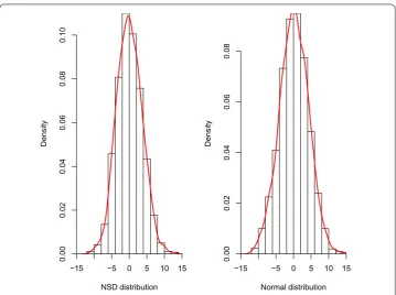
Firstly, we generate a NSD sequence by the Gibbs sampling technique. Figure shows the fitted distribution (full line) of NSD is close to the normal distribution, relatively speaking, the NSD distribution tends to behave a truncated distribution feature.
Next, we evaluate the estimators of regression coefficients and redundancy parameters under the null hypothesis, Table illustrates that the M-methods are valid (the corre-sponded M-estimates are close to true parametersβ= ,β= ) and the estimators of
redundancy parameters are effective (one may easily to check thatσ= andλ= when
Figure 1 Histograms and fitted distributions of M-estimates residuals with different explanatory variables and M-methods (sample size isn= 1,000).
Table 1 The evaluations of regression coefficients and redundancy parameters
Estimates n LS LAD Huber
I II I II I II
ˆ
β0 100 1.031 0.985 1.016 0.978 1.006 1.007
500 0.994 0.994 1.008 1.006 1.003 1.006
1000 1.002 0.999 1.000 1.006 1.002 1.003
ˆ
β1 100 1.983 2.008 1.992 2.016 2.131 2.131
500 2.003 2.011 1.997 2.003 1.996 1.992
1000 1.997 1.997 1.999 1.998 1.996 1.994
ˆ σ2
n 100 12.764 12.671 0.984 0.987 9.095 9.100
500 12.965 12.941 0.997 0.997 9.193 9.206
1000 12.967 12.956 0.998 0.998 9.208 9.291
ˆ
λn 100 1.000 1.000 0.282 0.282 0.825 0.825
500 1.000 1.000 0.241 0.241 0.822 0.823
1000 1.000 1.000 0.233 0.234 0.822 0.821
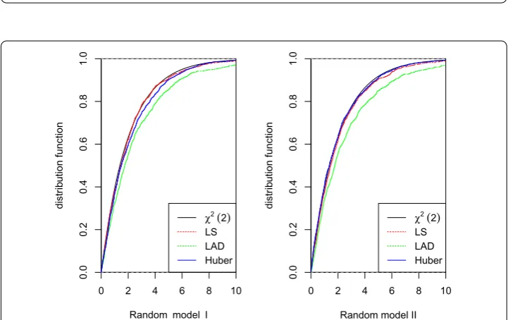
to the assumed NSD errors in Figure , and all of them still show a truncated distribu-tion feature. Figure checks the residuals are NSD by using the empirical distribudistribu-tion to approximate the distribution function, which supports the NSD errors assumption.
[image:18.595.118.479.410.574.2]Figure 2 Histograms and fitted distributions of M-estimates residuals with different explanatory variables and M-methods (sample size isn= 1,000).
Table 2 The powers of the M-test with NSD errors, ‘∗’ is for the nominal significant levels
n Significance levels
LS LAD Huber
I II I II I II
100 0.05∗ 0.063 0.068 0.082 0.079 0.062 0.062
0.01∗ 0.013 0.011 0.028 0.019 0.013 0.016
500 0.05∗ 0.059 0.057 0.064 0.052 0.054 0.059
0.01∗ 0.009 0.013 0.020 0.013 0.009 0.012
1000 0.05∗ 0.056 0.056 0.062 0.052 0.048 0.057
0.01∗ 0.012 0.015 0.013 0.011 0.010 0.013
illustrates that λˆnσˆnMncan approximate the centralχwell by comparing the empirical
distributions of λˆnσˆnMnwithχ, which implies that the M-test is valid under the local
alternatives.
5 Conclusions
[image:19.595.117.478.489.586.2]Figure 3 A comparison fitted distribution functions of residuals and assumed NSD errors (sample size isn= 1,000).
Figure 4 A comparison fitted distribution functions of 2λˆnσˆn2Mnand the central chi-squared
distribution with two degrees (sample size isn= 1,000).
Acknowledgements
This work is supported by Natural Science Foundation of China (No. 11471105; 61374183; 11471223), and Science and Technology Research Project of Education Department in Hubei Province of China (No. Q20172505).
Competing interests
The authors declare that they have no competing interests.
Authors’ contributions
All authors contributed equally to the writing of this paper. All authors read and approved the final manuscript.
Author details
1State Key Laboratory of Mechanics and Control of Mechanical Structures, Institute of Nano Science and Department of
Mathematics, Nanjing University of Aeronautics and Astronautics, Nanjing, 210016, China.2Department of Mathematics
and Statistics, Hubei Normal University, Huangshi, 435002, China.3Department of Information Science and Technology,
[image:20.595.117.478.300.527.2]Publisher’s Note
Springer Nature remains neutral with regard to jurisdictional claims in published maps and institutional affiliations.
Received: 26 December 2016 Accepted: 26 August 2017 References
1. Huber, PJ: Robust Statistics. Wiley, New York (1981)
2. Bai, ZD, Rao, CR, Wu, Y: M-estimation of multivariate linear regression parameters under a convex discrepancy function. Stat. Sin.2, 237-254 (1992)
3. Elsh, AH: Bahadur representations for robust scale estimators based on regression residuals. Ann. Stat.14, 1246-1251 (1986)
4. Yohai, VJ: Robust estimation in the linear model. Ann. Stat.2, 562-567 (1974)
5. Yohai, VJ, Maronna, RA: Asymptotic behavior of M-estimators for the linear model. Ann. Stat.7, 258-268 (1979) 6. Berlinet, A, Liese, F, Vajda, I: Necessary and sufficient conditions for consistency of M-estimates in regression models
with general errors. J. Stat. Plan. Inference89, 243-267 (2000)
7. Cui, HJ, He, XM, Ng, KW: M-estimation for linear models with spatially-correlated errors. Stat. Probab. Lett.66, 383-393 (2004)
8. Wu, WB: M-estimation of linear models with dependent errors. Ann. Stat.35, 495-521 (2007)
9. Wu, QY: The strong consistency of M estimator in a linear model for negatively dependent random samples. Commun. Stat., Theory Methods40, 467-491 (2011)
10. Hu, TZ: Negatively superadditive dependence of random variables with applications. Chinese J. Appl. Probab. Statist. 16(2), 133-144 (2000)
11. Wang, XJ, Shen, AT, Chen, ZY: Complete convergence for weighted sums of NSD random variables and its application in the EV regression model. Test24, 166-184 (2015)
12. Christofides, TC, Vaggelatou, E: A connection between supermodular ordering and positive/negative association. J. Multivar. Anal.88(1), 138-151 (2004)
13. Nelsen, RB: An Introduction to Copulas. Springer, New York (2006)
14. Jaworski, P, Durante, F, Härdle, WK: Copulas in Mathematical and Quantitative Finance. Springer, Heidelberg (2013) 15. Eghbal, N, Amini, M, Bozorgnia, A: Some maximal inequalities for quadratic forms of negative superadditive
dependence random variables. Stat. Probab. Lett.80, 587-591 (2010)
16. Eghbal, N, Amini, M, Bozorgnia, A: On the Kolmogorov inequalities for quadratic forms of dependent uniformly bounded random variables. Stat. Probab. Lett.81, 1112-1120 (2011)
17. Shen, AT, Zhang, Y, Volodin, A: Applications of the Rosenthal-type inequality for negatively superadditive dependent random variables. Chemom. Intell. Lab. Syst.78, 295-311 (2015)
18. Wang, XJ, Deng, X, Zheng, LL, Hu, SH: Complete convergence for arrays of rowwise negatively superadditive dependent random variables and its applications. Statistics48, 834-850 (2014)
19. Wang, XH, Hu, SH: On the strong consistency of M-estimates in linear models for negatively superadditive dependent errors. Aust. N. Z. J. Stat.57(2), 259-274 (2015)
20. Zhao, LC, Chen, XR: Asymptotic behavior of M-test statistics in linear models. J. Comput. Inf. Syst.16, 234-248 (1991) 21. Chen, XR, Zhao, LC: M-Methods in Linear Model. Shanghai Sci. Technol., Shanghai (1996)
22. Bai, ZD, Rao, CR, Zhao, LC: MANOVA type tests under a convex discrepancy function for the standard multivariate linear model. J. Stat. Plan. Inference36, 77-90 (1993)
23. Rao, CR: Tests of significance in multivariate analysis. Biometriks35, 58-79 (1948)
24. Rao, CR, Zhao, LC: Linear representation of M-estimates in linear models. Can. J. Stat.20, 359-368 (1992) 25. Zhao, LC: Strong consistency of M-estimates in linear models. Sci. China Ser. A45(11), 1420-1427 (2002) 26. Bai, ZD, Rao, CR, Wu, Y: M-estimation of multivariate linear regression parameters under a convex discrepancy
function. Stat. Sin.2, 237-254 (1992)
27. Newman, CM: Normal fluctuations and the FKG inequalities. Commun. Math. Phys.74, 119-128 (1980) 28. Liang, HY, Jing, BY: Asymptotic properties for estimates of nonparametric regression models based on negatively
associated sequences. J. Multivar. Anal.95(2), 227-245 (2005)
29. Yu, YC, Hu, HC: A CLT for weighted sums of NSD random sequences and its application in the EV regression model. Pure Appl. Math.32(5), 525-535 (2016)
30. Hu, HC, Pan, X: Asymptotic normality of Huber-Dutter estimators in a linear EV model with AR(1) processes. J. Inequal. Appl.2014(1), 474 (2014)
31. Anderson, PK, Gill, RD: Cox’s regression model for counting processes: a large sample study. Ann. Stat.15, 1100-1120 (1982)