AK P: An Active Learning Method Combing Kriging and Probability Density Function for Reliability Analysis

2018 International Conference on Applied Mechanics, Mathematics, Modeling and Simulation (AMMMS 2018) ISBN: 978-1-60595-589-6

AK-P: An Active Learning Method Combing Kriging and Probability

Density Function for Reliability Analysis

Cheng-ning ZHOU

, Ning-cong XIAO

, Ming J. ZUO

and Mei CHEN

1_{School of Mechanical and Electrical Engineering,}

University of Electronic Science and Technology of China, Chengdu, Sichuan, P. R. China

2_{Department of Mechanical Engineering, University of Alberta,} Edmonton, Alberta, T6G1H9, Canada

*Corresponding author

Keywords: Reliability analysis, Kriging model, Probability density function, Active learning.

Abstract. An important challenge in structural reliability is to reduce the number of calls to the performance function. To reduce computational burden, surrogate models are commonly used. Kriging, one of the meta-models, is widely used as a surrogate for the original model in structural reliability analysis. In this paper, an active learning method combing Kriging and probability density function is proposed to improve the computational efficiency of AK-MCS. The proposed method, in general, provides a more efficient way by selecting the next best point effectively and adding it to the design of experiments to update the surrogate model more accurately. One example is used to demonstrate the efficiency of the proposed method.

Introduction

It is important to assess the probability of failure for a given mechanical structure considering the randomness of input variables. Generally, the probability of failure is defined as

( ) 0 ( ) ,

f G

P 



(1)

where 𝑓(𝒙) is the joint probability density function (PDF) of input variables X, and 𝐺(∙) is the performance function of analyzed mechanical structure. The variable space is divided by the limit state (𝐺(𝒙) = 0) into two domains, i.e., the failure domain (𝐺(𝒙) ≤ 0) and the safe domain (𝐺(𝒙) > 0).

The probability of failure in Eq.1 can also be described as follows:

( ) ( ) ,

f G x

P 



(2)

where 𝐼_𝐺≤0 is a failure indicator function that is defined as:

( )

1 ( ) 0

.

0 ( ) 0

G x

G I

G

 

  _



x

x (3)

( ) 0

ˆ _,

f n_G P

N_MC



 x

(4)

the samples located in the failure domain (G(𝐱) ≤ 0). For small failure probability events, NMC should be large enough in order to get a convergent result, i.e., N_MC= (102~104)/P_f [3]. Problems analyzed in engineering about structural reliability always have very small probability, and N_MC should be large enough. Especially, the performance function is usually implicit and the finite element model (FEM) is utilized to get the response, which is time-consuming.

To reduce the total calls to the performance function and relieve the pressure of computation, some variance reduction techniques were proposed, e.g., subset simulation (SS) [4-6], important sampling (IS) [7, 8], and line sampling (LS) [9]. SS computes the failure probability as a product of a series of conditional probabilities estimated easily by Markov Chain Monte Carlo (MCMC) simulation [10].The basic principle of IS is to generate points around the most probable point (MPP) that reside around the vicinity of the limit state surface. Although IS is one of the most effective variance reduction techniques, its success depends on the prior knowledge about the failure domain and the auxiliary distribution assignment [11]. LS computes the probability of failure based on the optimal important direction which is from the origin of coordinate to MPP in the standard normal space [9]. These variance reduction techniques effectively improve the efficiency of computation through a reduced number of calls to the performance function compared to MCS. However, these variance reduction technologies are difficult when applied to the engineering structural reliability problems with FEM models.

Constructing a model to substitute the complex performance function has been a key research thrust. In recent years, many machine learning methods are proposed to construct the substituted model in structural reliability problems, e.g., neural networks [12-14], support vector machines (SVM) [15, 16]. These machine learning methods are more suitable to matching performance function with highly nonlinear input-output relationships [17]. Kriging, one of the machine learning methods, is widely used as a surrogate for the original model in structural reliability analysis [3, 8, 18-22], which presents interesting characteristics such as exact interpolation and a local index of uncertainty on the prediction. Therefore, the Kriging model is employed combing with probability density function in this research.

The paper is organized as follows. Section II reviews the basic theory of Kriging method. Section III presents AK-P: a new active learning method combing Kriging and probability density function. Section IV presents the implementation progress of reliability analysis by the proposed active learning method AK-P. One example is employed in section V to illustrate the efficiency of the proposed method. Section VI is the conclusion.

Basic Theories of Kriging for Structural Reliability Analysis

Kriging developed the Kriging approach for geo-statistics, and Matheron refined this surrogate model [23]. The Kriging model includes two parts: a linear regression model and a stochastic process [24]:

ˆ ( ) T( ) ( ), G x  f x Z x

(5)

where F(𝒙, β) is the deterministic part and Z(𝒙) is a stationary Gaussian process with zero mean, and the covariance between two points can be defined as

2

ov( ( ), ( )) ( , ), , 1, 2,..., C Z x_i Z x_j  R x x_{i j} i j N

(6)

A New Active Learning Method

Learning Function

The learning function is used to find the next best point in the random space including learning criterion and stop condition, and then the point will be added to the design of experiments (DoE) to update the Kriging model more accurately.

EFF (Expected feasibility function) is proposed by Bichon [26], and is defined as

ˆ

ˆ_{( )} G _{( )} ˆ_{( )} ˆ_, G G

EFF G  G G f dG





     

 

 x   x x  (7)

where 𝐺̅(𝒙) is the constraint equation and 𝑓_𝐺̂ is the PDF of 𝐺̂(𝒙). 𝜀 = 𝑘𝜎_Ĝ(𝑥), and 𝑘 is always equal to 2. To guarantee the accuracy near the limit state function,𝐺− = 𝐺̅(𝒙) − 𝜀, 𝐺+ = 𝐺̅(𝒙) + 𝜀. In reliability analysis, 𝐺̅(𝑥) = 0.

However, this learning function approximates the whole limit state which causes a slow convergence.

Table 1. Definition of the learning criterion and the stipping condition for the learning functions EFF and U.

Learning function EFF U

Learning criterion max(EFF(x)) min(U(x))

Stop condition max(EFF(𝒙)) ≤ 0.001 min(U(𝒙)) ≥ 2

The learning function U is proposed by Echard [18] as,

ˆ

ˆ ( ) ( ) ( ) 0, G G x U x x 

(8)

According to Eq.8, higher weight is applied to the points in the close neighborhood of the predicted limit state rather than further ones with high Kriging variance like EFF can do.

Table 1 sums up the learning parameters for EFF and U [18].

Principles of the Proposed Methodology

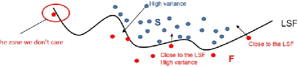
Figure 1. Three characteristics of points in a small value of U function.

In this paper, a new learning function named AK-P is proposed to combing Kriging and probability density function for reliability analysis.

If the U function value is low, the sample point corresponding to the U function shows three characteristics: 1. The sample point is close to the limit state. 2. The sample point with a higher prediction variance has an important uncertainty than others. 3. The sample points has the characteristics presented in 1 and 2 that is shown in Fig. 1 (S and F stand for safe region and failure region, respectively).

If these points which have a low probability density as well as a small value of U that are added to the DoE, the number of calls to the performance function will increase, while the accuracy of final estimation of failure probability has no obvious improvement. To improve the efficiency of reliability analysis, the points with the probability density function and the value of U are not considered.

model in a mojire effective way. The sample points selected not only have a low U value, but also have a relative large probability density. The new learning function 𝑈∗(𝑋) is defined as:

*

min ( ), 1, 2, ..., , ( )

L

L

L

U

U L N

f

 x 

x (9)

where 𝑈(𝑋) is obtained by AK-MCS, and 𝑓(𝑋) is the joint probability density function of the input random variables. The inverse function of the PDF of the input random variables shows that the larger the PDF, the lower the learning function. The point with the minimum U* value in the random variables space will be selected.

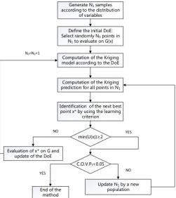
The learning method based on AK-MCS for the reliability problems can be performed as Fig. 2:

Procedure of the Propose Method

Generate N1 samples according to the distribution

of variables

Define the initial DoE: Select randomly N0 points in

N1 to evaluate on G(x)

Computation of the Kriging model according to the DoE

Computation of the Kriging prediction for all points in N1

Identification of the next best point x* by using the learning

criterion

min(U(x))2

C.O.V.Pf<0.05

End of the method Evaluation of x* on G and

update of the DoE

Update N1 by a new population

NO YES

YES NO

N0=N0+1

Figure 2. Flow chart of the proposed method.

The details of proposed methodology can be explained as follows:

a) Construction of the initial Kriging model: Generate N₁ samples according to the distribution of variables, and select randomly N₀ points in N₁ to construct an initial Kriging model.

b) Computation of the Kriging prediction of all candidate sample points and find the next best point: Compute the predictions of all sample points utilizing the Kriging model constructed in Step a. Find the next best point according to the proposed method described in Section 3.

c) Convergence criterion judgment: Estimate the value of learning function U and determine whether the convergence criterion is met. If criterion is not met, add the next best point and its response to the DoE, and go to Step b to improve the accuracy of the Kriging model. If else, go to next step.

d) Estimation of the probability of failure: Compute the probability of failure based on the predictions obtained in Step b using MCS method. If the coefficient of variation is low enough, the proposed method stops, and the last estimation of failure probability is considered as the result of the reliability analysis. If not, go to Step a and start the process again.

Numerical Examples

installed on a computer with an Intel Core i7-6700, a 8.00 GB RAM, and an operation system of Windows 10 enterprise edition.

A Highly Nonlinear Two-Dimensional Example

A highly nonlinear performance function [27] is defined by

2

1 1 2

5 ( 4)( 1)

( ) sin 2 ,

2 20

x x x

G x     

(10)

where 𝑥1 and 𝑥2 are two independently and normally distributed random variables with

𝑥₁~𝑁(1.5,1) and 𝑥₂~𝑁(2.5,1).

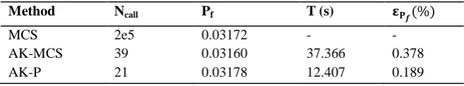
The comparisons of AK-MCS, MCS and proposed method AK-P are given in Table 2. The probability of failure obtained by MCS is used as the reference. To assess the accuracy of AK-MCS based on the learning function U and the proposed method, 12 sample points are randomly selected by MCS as the initial DoE for the Kriging process, and 2 × 105 points are generated randomly according to the distributions of the random variables as the candidate sample points for the selection of next best point.

T is the CPU time of the program measured in seconds. The smaller the T, the higher the efficiency. The probability of failure obtained by AK-P is almost the same as the results from the AK-MCS, while the computational efficiency is higher than AK-MCS in this paper. Some details are shown in Fig. 3 and Fig. 4, respectively. LSF is short for limit state function. Fig. 4 illustrates the proposed method puts more weight in the region with a higher probability density in reliability analysis compared to Fig. 3. As shown in Fig. 3 and Fig. 4, the sample points added to the DoE in the method AK-P are centered more on the region with a large value of PDF, while the points are relatively scattered in the method AK-MCS.

Figure 3. The result of example 1 obtained by AK-MCS. Figure 4. The result of example 1 obtained by AK-P.

Table 2. Reliability results of example 1.

Method Ncall Pf T (s) 𝛆𝐏_𝒇(%)

MCS 2e5 0.03172 - -

AK-MCS 39 0.03160 37.366 0.378

AK-P 21 0.03178 12.407 0.189

Conclusion

proposed method is generally more accurate and efficient than the AK-MCS with learning function U. However, it does not mean that the proposed method is more efficient than AK-MCS for all cases. The main reasons is that the updated Kriging model selects the next best point avoid the area with small probability using the proposed learning function. The proposed method can be a useful tool for reliability analysis, especially for problems with complex implicit limit state functions.

Acknowledgment

This work was supported by the National Natural Science Foundation of China (Nos. 11602054 and 51537010) and the Natural Sciences and Engineering Research Council of Canada (Grant #RGPIN-2015-04897).

References

[1] G. S. Fishman, Monte Carlo: Springer New York, 1996.

[2] B. Gaspar, A. Naess, B. J. Leira, and C. G. Soares, “System Reliability Analysis by Monte Carlo Based Method and Finite Element Structural Models,” Journal of Offshore Mechanics & Arctic Engineering, vol. 136, p. 031603, 2014.

[3] L. Zhang, Z. Lu, and P. Wang, “Efficient structural reliability analysis method based on advanced Kriging model,” Applied Mathematical Modelling, vol. 39, pp. 781-793, 2015.

[4] S. K. Au and J. L. Beck, “Estimation of small failure probabilities in high dimensions by subset simulation,” Probabilistic Engineering Mechanics, vol. 16, pp. 263-277, 2001.

[5] X. Huang, J. Chen, and H. Zhu, “Assessing small failure probabilities by AK–SS: An active learning method combining Kriging and Subset Simulation,” Structural Safety, vol. 59, pp. 86-95, 2016.

[6] H. S. Li and S. K. Au, “Design optimization using Subset Simulation algorithm,” Structural Safety, vol. 32, pp. 384-392, 2010.

[7] R. E. Melchers, “Importance sampling in structural system,” Structural Safety, vol. 6, pp. 3-10, 1989.

[8] B. Echard, N. Gayton, M. Lemaire, and N. Relun, “A combined Importance Sampling and Kriging reliability method for small failure probabilities with time-demanding numerical models,” Reliability Engineering & System Safety, vol. 111, pp. 232-240, 2013.

[9] Z. Lv, Z. Lu, and P. Wang, “A new learning function for Kriging and its applications to solve reliability problems in engineering,” Computers & Mathematics with Applications, vol. 70, pp. 1182-1197, 2015.

[10]X. Descombes, R. Morris, J. Zerubia, and M. Berthod, “Maximum Likelihood Estimation of Markov Random Field Parameters Using Markov Chain Monte Carlo Algorithms,” in International Workshop on Energy Minimization Methods in Computer Vision and Pattern Recognition, pp. 133-148, 1997.

[11]L. Li, J. Bect, and E. Vazquez, “Bayesian Subset Simulation: a kriging-based subset simulation algorithm for the estimation of small probabilities of failure,” Statistics, 2012.

[13]J. B. Cardoso, J. R. De Almeida, J. M. Dias, and P. G. Coelho, “Structural reliability analysis using Monte Carlo simulation and neural networks,” Advances in Engineering Software, vol. 39, pp. 505-513, 2008.

[14]J. Cheng, Q. S. Li, and R. Xiao, “A new artificial neural network-based response surface method for structural reliability analysis,” Probabilistic Engineering Mechanics, vol. 23, pp. 51-63, 2008.

[15]H. Song, K. K. Choi, I. Lee, L. Zhao, and D. Lamb, “Adaptive virtual support vector machine for reliability analysis of high-dimensional problems,” Structural & Multidisciplinary Optimization, vol. 47, pp. 479-491, 2013.

[16]U. Alibrandi, A. M. Alani, and G. Ricciardi, “A new sampling strategy for SVM-based response surface for structural reliability analysis,” Probabilistic Engineering Mechanics, vol. 41, pp. 1-12, 2015.

[17]Z. Sun, J. Wang, R. Li, and C. Tong, “LIF: A new Kriging based learning function and its application to structural reliability analysis,” Reliability Engineering & System Safety, vol. 157, pp. 152-165, 2017.

[18]B. Echard, N. Gayton, and M. Lemaire, “AK-MCS: An active learning reliability method combining Kriging and Monte Carlo Simulation,” Structural Safety, vol. 33, pp. 145-154, 2011.

[19]B. Gaspar, A. P. Teixeira, and C. Guedes Soares, “Adaptive surrogate model with active refinement combining Kriging and a trust region method,” Reliability Engineering & System Safety, vol. 165, pp. 277-291, 2017.

[20]S. Song, “Structural Reliability Sensitivity Analysis Method Based on Markov Chain Monte Carlo Subset Simulation,” Journal of Mechanical Engineering, vol. 45, pp. 33, 2009.

[21]G. Xue, H. Dai, H. Zhang, and W. Wang, “A new unbiased metamodel method for efficient reliability analysis,” Structural Safety, vol. 67, pp. 1-10, 2017.

[22]Z. Peijuan, W. C. Ming, Z. Zhouhong, and W. Liqi, “A new active learning method based on the learning function U of the AK-MCS reliability analysis method,” Engineering Structures, vol. 148, pp. 185-194, 2017.

[23]G. Matheron, “The intrinsic random functions and their applications,” Advances in Applied Probability, vol. 5, pp. 439-468, 1973.

[24]J. Sacks, S. B. Schiller, and W. J. Welch, “Designs for Computer Experiments,” Technometrics, vol. 31, pp. 41-47, 1989.

[25]Kaymaz, “Application of kriging method to structural reliability problems,” Structural Safety, vol. 27, pp. 133-151, 2005.

[26]B. J. Bichon, M. S. Eldred, L. P. Swiler, S. Mahadevan, and J. M. McFarland, “Efficient Global Reliability Analysis for Nonlinear Implicit Performance Functions,” AIAA Journal, vol. 46, pp. 2459-2468, 2008.