Numerical Solution for PDE-Constrained Optimization
Problem in Cardiac Electrophysiology
Kin Wei Ng
Department of Mathematical Sciences Faculty of Science
Universiti Teknologi Malaysia 81310 Johor Bahru, Malaysia
Ahmad Rohanin
Department of Mathematical Sciences Faculty of Science
Universiti Teknologi Malaysia 81310 Johor Bahru, Malaysia
ABSTRACT
In this paper, we present the numerical solution for the PDE-constrained optimization problem arises in cardiac electrophysiology. The monodomain model, which is a well-established model for simulating electrical behavior of the cardiac tissue, appears as the constraint in our problem. Our objective is to search for the optimal applied current, which is able to dampen out the excitation wavefront of the transmembrane potential during defibrillation process. The modified Dai-Yuan nonlinear conjugate gradient method is employed for computing the optimal applied current, and our numerical results show that the excitation wavefront is successfully dampened out by the optimal applied current.
General Terms
PDE-constrained optimization, Cardiac electrophysiology.
Keywords
Monodomain model, Operator splitting, Optimal control.
1.
INTRODUCTION
Sudden cardiac death is an unexpected death of a person in a short time period, and is often attributed to cardiac arrhythmias. During an arrhythmia, the heart may beat too slowly, too rapidly, or irregularly. There are many types of cardiac arrhythmia, and the most common life-threatening arrhythmia is ventricular fibrillation. Currently, the only effective therapy for termination of ventricular fibrillation is through electrical defibrillation [1, 2]. However, there are some adverse effects associated with defibrillation such as myocardial dysfunction and damage [3]. In the effort of minimizing the adverse effects, it is essential to determine the minimal current required for successful defibrillation. As a result, the optimal defibrillation process can be formulated as a PDE-constrained optimization problem, in which the monodomain model appears as the constraint.
The monodomain model is a well-established mathematical model for numerical simulation of cardiac electrical activity [4, 5]. It consists of a parabolic partial differential equation (PDE) coupled with a system of nonlinear ordinary differential equations (ODEs) representing cell ionic activity. In the context of optimally controlled defibrillation process, it is essential to determine the optimal applied extracellular current, which is able to drive the heart rhythm back to normal. In other words, we are trying to search for the optimal current in such a way that it dampens the excitation wavefront of the transmembrane potential during defibrillation process. The main purpose of this paper is therefore to provide a numerical solution for the optimal control problem of the monodomain model.
The structure of the paper is organized as follows. Section 2 presents the optimal control problem of the monodomain model with Rogers-Modified FitzHugh-Nagumo ion kinetic. The numerical approach used to solve the optimal control problem is discussed in Section 3, while the optimization algorithm is presented in Section 4. Next, the numerical results are given in Section 5. Finally, we conclude our paper with a short discussion in Section 6.
2.
OPTIMAL CONTROL PROBLEM
Let 2 denotes the computational domain, c
denotes the control domain and o denotes the observation domain. The optimal control problem for monodomain model is given by
on , 0 ,
on , 0 ,
, 0 on , 0
, 0 in , 0
, 0 in , 0
s.t.
2 1 , min
0 0
0
2 2
x w x w
x V x V
T V
D
T f
t w
T I
I t V C V D
dt d I d
V I
V J
ion m
T
c e o
e
o c
(1)
where
e
i I
λ I D
D
1 1 and 1
Here 0 is a regularization parameter, T is final simulated time and is unit normal vector directed outwards from . Moreover, Di is intracellular conductivity tensor,
is surface-to-volume ratio of the cell membrane, Cm is
membrane capacitance per unit area, Iion
V,w
is current density flowing through the ionic channels, f
V,w
is prescribed vector-value functions, is a constant scalar used to relate the intracellular and extracellular conductivity tensors, V
x,t is transmembrane potential, w
x,t are ionic current variables and Ie
x,t is extracellular current density stimulus. Both functions Iion
V,w
and f
V,w
depend on the ionic model. In this paper, we adopt Rogers-Modified FitzHugh-Nagumo model [6] which is given by
c wVV V V
V V c w V
Iion , 1 1 1 2
cw
V V c w V f p 4 3 ,
Here Vp is plateau potential, Vth is threshold potential, and
4 3 2 1,c ,c,c
c are positive parameters. Notice that the optimal control problem in (1) is a PDE-constrained optimization problem with V and w as the state variables, and Ie as the control variable. The control variable is chosen such that it is nontrivial only within the control domain. Also, the control variable is chosen in the best possible way to achieve our control objective, which is to dampen out the excitation wavefront of transmembrane potential in the observation domain.
3.
NUMERICAL APPROACH
3.1
First Order Optimality System
We adopt the optimize-then-discretize approach to solve the optimal control problem in (1). For deriving the first order optimality system, Lagrange functional, L, is formed.
dt d q f t w dt d p I I t V C V D dt d I d V T T ion m T c e o o c
2 1 0 0 0 2 2 L (2)where p
x,t and q
x,t are Lagrange multipliers which are used to adjoin the constraints to the cost functional. The first order optimality system is obtained by setting the partial derivatives of (2) equal to zero. As a result, the first order optimality system consists of the following:
, 0 , and 0 , , 0 , , 0 0 x wx w xV x V V D f t w I I V D t V
Cm ion
(3)
, 0 , and 0 , , 0 , , T x q T x p p D q f p I t q V q f p I p D t p C w w ion o V V ion m (4)
T pIe 0, in c 0, 1
1
(5)
where
denotes the partial derivative with respect to ando
V denotes the transmembrane potential in the observation domain. Here, (3) is known as state system, (4) is known as adjoint system and (5) is the optimality condition.
According to [7], the control-to-state mapping
e e
e V I wI
I
C , is well-defined. Thus, the cost functional,J
V,Ie
, in (1) can be rewritten as
I V
I d I d dtJ T c e o e e o c
0 2 2 2 1 ˆ where Jˆ
Ie is known as reduced cost functional. Furthermore, the gradient of the reduced cost functional is given as
I I pJ e e
1 1 ˆ
3.2
Numerical Discretization
To complete the optimize-then-discretize approach, the optimality system needs to be discretized. In order to reduce the complexity of the optimality system, the operator splitting technique [8] is applied to split (3) and (4) into smaller parts that are easier to solve. After applying the operator splitting technique, the nonlinear PDE in (3) is split into a linear PDE and a nonlinear ODE as follows
D V
t V
Cm I I t V
Cm ion
Similarly, the nonlinear PDE in (4) becomes
D p
t p
Cm
ionV
V om I p f q V
t p
C
For the discretization procedure, the linear PDEs are discretized with Galerkin finite element method in space and Crank-Nicolson method in time. On the other hand, the nonlinear ODEs are discretized with forward Euler method in time. The discretized state system is therefore given as
, 0 , , 0 , , , 2 2 2 1 2 1 1 1 1 x x x x t C C t t C t C n n n m n m n n n n m n m 0 0 ion w w V V f w w I I V V V K M V K M (6)and the discretized adjoint system is given as
, , , , , 2 2 1 1 1 1 2 1 1 1 1 1 1 2 1 1 1 1 0 q 0 p q f p I q q q f p I V p p p K M p K M ion ion T x T x t C C C t t C t C n w n n w n n n n m V n n m V n m o n n n n m n m (7)4.
OPTIMIZATION ALGORITHM
The nonlinear conjugate gradient method is an attractive method for solving large-scale unconstrained optimization problem due to its simplicity and low memory requirements [9, 10]. For the previous work, Nagaiah et. al. [11] applied the Dai-Yuan (DY) nonlinear conjugate gradient method [12] for solving the optimal control problem of the monodomain model. For this paper, the modified Dai-Yuan (MDY) method [13] is employed. MDY method is chosen because it not only inherits all the nice properties of DY method, but also proven to converge globally, independent of the line search used. The algorithm for solving the discretized optimal control problem is shown as follows.
Overall Solution Algorithm:
Step 0. Provide an initial guess I0e and set k0.
Step 1. Set V
x,0 V0
x and w
x,0 w0
x . Solve the discretized state system (6).Step 2. Evaluate the reduced cost functional Jˆ . k Step 3. Set p
x,T 0 and q
x,T 0. Use the resultobtained in Step 1 to solve the discretized adjoint system (7).
Step 4. Update the gradient Jk Iek pk
1 1
ˆ .
Step 5. For k1, check the stopping criteria
4 1
10 ˆ ˆk k
J
J and Jˆk 104
1 Jˆk If one of them is met, then stop.Step 6. Compute
, 1 ,
ˆ
, 0 ,
ˆ
1
k if
k if
k k k k k
d J
J d
where
1
1 1 1
2
ˆ ˆ
ˆ
k k k k k T k
k k
d J
J d
J
2 1 1
1 1
1 2
3 ˆ ˆ
, 0 max ˆ
10
k k
k k T k k k
k
d J J d J
Step 7. Compute step-length k using Armijo line search.
Step 8. Update the control variable Iek Ikekdk
1
. Set
1
k
k and go to Step 1.
5.
NUMERICAL EXPERIMENTS
5.1
Experiments Setup
The numerical experiments are carried out on a two-dimensional computational domain
0,10,1 of size2
cm 1
1 for T3mssimulation time. Two control domains are considered, namely c1
0.375,0.438
0.469,0.531
domain is defined as the complement of neighborhoods of
1
c
and c2. By taking
0.359,0.453
0.453,0.547
~
1
c
and ~c2
0.547,0.641
0.453,0.547
as the neighborhoods of the control domains, the observation domain is therefore given as o\
~c1~c2
. The excitation domain is the region where cardiac arrhythmia first occurs, and is denoted as exi
0.498,0.502
0.498,0.504
o. The observation [image:3.595.321.534.187.378.2]domain and the control domain are shown in Figure 1.
Fig 1: The control and observation domains
Table 1 lists the parameters that we have used in our numerical experiments, with some of them adopted from [14]. Furthermore, the initial conditions for V, Ie and ware given as
otherwise,
mV, 0
, mV, 105 0
, x exi
x V
otherwise,
, cm mA 0
, , cm mA 0 0 ,
3 3
c e
x x
I
x x [image:3.595.310.548.571.764.2]w ,0 0,
Table 1. Parameters used in numerical experiments
Parameter Value Units
3
10 cm1
m
C 3
10 mFcm2
l i
D 3
10
3 Scm1
t i
D 4
10 1525 .
3 Scm1
th
V 1
10 3 .
1 mV
p
V 2
10 mV
1
c 1.5 2
cm mS
2
c 4.4 2
cm mS
3
c 2
10 2 .
1 ms1
4
c 1 dimensionless
4
10 dimensionless
5.2
Numerical Results
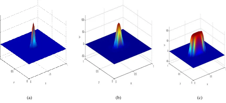
In this section, we present the numerical results for the optimal control problem of the monodomain model. The uncontrolled solutions and the optimally controlled solutions at times 0.2 ms, 1 ms and 3 ms are illustrated in Figure 2 and Figure 3. Numerical results show the uncontrolled wavefront
of the transmembrane potential spreads from the excitation domain to the rest of the computational domain if no action for controlling is carried out. On the other hand, when the control is switched on, the excitation wavefront is successfully dampened out by the optimal applied current
opt e
I during the time interval from 0 ms to 3 ms.
[image:4.595.74.506.158.355.2](a) (b) (c)
Fig 2: The uncontrolled solutions
V at (a) 0.2 ms (b) 1 ms and (c) 3 ms(a) (b) (c)
Fig 3: The controlled solutions
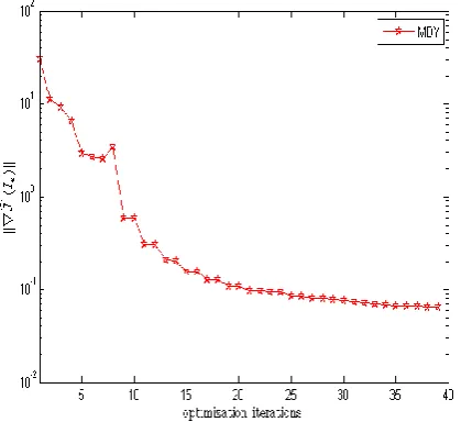
Vopt at (a) 0.2 ms (b) 1 ms and (c) 3 msNext, we discuss the performance of MDY method for solving the optimal control problem of monodomain model. Figure 4
depicts the minimum value of the reduced cost functional Jˆ
Ie along the optimization process. As shown in the figure, the MDY method converges to the minimizer with 38 optimization iterations. Unlike the DY method which descent property depends on the line search [13], the MDY method is well-performed even if the Armijo line search is used in our numerical experiments.Figure 5 depicts the corresponding norm of gradient of the
[image:4.595.68.524.398.597.2]Fig 4: Minimum value of Jˆ for 3 ms of simulation time
Fig 5: Norm of gradient of Jˆ for 3 ms of simulation time
6.
CONCLUSIONS
In this paper, we have presented the numerical solution for the optimal control problem of monodomain model using the MDY method. Our numerical results indicated that the excitation wavefront of the transmembrane potential has been successfully dampened out by the optimal applied current. Numerical results also indicated that the MDY method perform quite well under Armijo line search. These results motivate us to continue our numerical experiments with different locations and sizes of the control domains using the MDY method.
7.
ACKNOWLEDGMENTS
The work is financed by Zamalah Scholarship provided by Universiti Teknologi Malaysia and the Ministry of Higher Education of Malaysia.
8.
REFERENCES
[1] Dosdall, D. J., Fast, V. G., and Ideker, R. E. 2010. Mechanisms of defibrillation. Annu. Rev. Biomed. Eng. 12, 233-258.
[2] Amann, A., Tratnig, R., and Unterkofler, K. 2005. A new ventricular fibrillation detection algorithm for automated external defibrillators. Comput. Cardiol. 32, 559-562.
[3] Runsiö, M., Kallner, A., Källner, G., Rosenqvist, M., and Bergfeldt, L. 1997. Myocardial injury after electrical therapy for cardiac arrhythmias assessed by troponin-T release. Am. J. Cardiol. 79, 1241-1245.
[4] Belhamadia, Y., Fortin, A., and Bourgault, Y. 2009. Towards accurate numerical method for monodomain models using a realistic heart geometry. Math. Biosci. 220, 89-101.
[5] Nagaiah, C. and Kunisch, K. 2011. Higher order optimization and adaptive numerical solution for optimal control of monodomain equations in cardiac electrophysiology. Appl. Numer. Math. 61, 53-65.
[6] Rogers, J. M. and McCulloch, A. D. 1994. A collocation-Galerkin finite element model of cardiac action potential propagation. IEEE Trans. Biomed. Eng. 41, 743-757.
[7] Kunisch, K. and Wagner, M. 2012. Optimal control of the bidomain system (I): The monodomain approximation with the Rogers-McCulloch model. Nonlinear Anal. RWA. 13, 1525-1550.
[8] Qu, Z. and Garfinkel, A. 1999. An advanced algorithm for solving partial differential equation in cardiac conduction. IEEE Trans. Biomed. Eng. 46(9), 1166-1168.
[9] Zhou, A., Zhu, Z., Fan, H., and Qing, Q. 2011. Three new hybrid conjugate gradient methods for optimization. Appl. Math. 2, 303-308.
[10] Chen, Y. 2012. Global convergence of a new conjugate gradient method with Wolfe type line search. J. Inf. Comput. Sci. 7(1), 67-71.
[11] Nagaiah, C., Kunisch, K., and Plank, G. 2011. Numerical solution for optimal control of the reaction-diffusion equations in cardiac electrophysiology. Comput. Optim. Appl. 49, 149-178.
[12] Dai, Y. H. and Yuan, Y. 1999. A nonlinear conjugate gradient method with a strong global convergence property. SIAM J. Optim. 10, 177-182.
[13] Zhang, L. 2009. Two modified Dai-Yuan nonlinear conjugate gradient methods. Numer. Algor. 50, 1-16.
[image:5.595.67.277.307.499.2]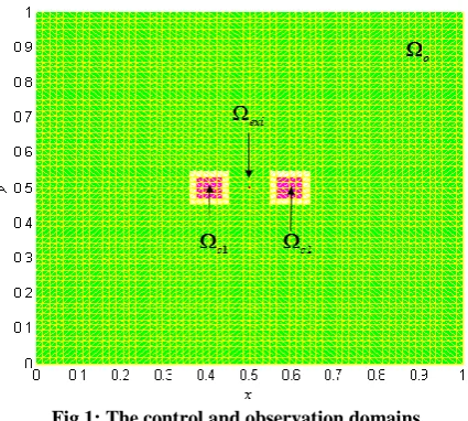
![Lexikologi som datalingvistik (Lexicology as computational linguistics) [In Swedish]](data:image/gif;base64,R0lGODlhAQABAIAAAP///wAAACH5BAEAAAAALAAAAAABAAEAAAICRAEAOw==)