Munich Personal RePEc Archive
THE ESTIMATION OF FOOD STAMP
SELF-SELECTION MODELS USING
THE METHOD OF SIMULATION
Keane, Michael and Moffitt, Robert
1992
CONTENTS
Chapter Page
EXECIYrIVE SUMMARY ... iv
I INTRODUCTION ... 1
II APPLYING THE MSM TO A MODEL OF MULTIPLE PROGRAM SELF-SELECTION ... 5
HI AN ILLUSTRATION WITH SIPP ... 10
IV SUMMARY... 20
TABLES
Table Pnge
Ill. 1 RF__ULTS OF THE ESTIMATION: 'ITIREE
PARTICIPATION EQUATIONS ONLY ... 12
1]].2 RESULTS OF THE ESTIMATION: THREE
PARTICIPATION EQUATIONS AND RENT EQUATION ... 14
1II.3 RUN TIMES FOR VARIOUS SPECIFICATIONS
OF THE MODEL ... 17
EXECUTIVE SUMMARY
An important issue associated with the Food Stamp Program (FSP) concerns the magnitude of its effects on the food expenditures, nutrition, and other outcomes of recipients. What must be considered in estimating the magnitudes of those effects is a well-known, but difficult, statistical problem arising from what is called "serf-selection" into the program. The problem arises when the effects of the program are gauged byacomparison of the outcomes of recipients to those of eligible nonrecipients. Such comparisons will be in error if the values of the outcomes observed for nonrecipients are not the same asthe outcomes that recipients would experience were they off the program. This discrepancy will occur if recipients are a "self-selected" group from the total population of eligibles. For example, if,as agroup, recipients would have lower food expenditures if they were off the program than current nonrecipients are observed to have, the observed difference in food expenditures between recipients and nonrecipients would either be too small, ifpositive, or possibly negative, and the estimated effect of the FSP would be biased.
While statistical solutions to this problem have been developed to be able to obtain correct comparisons for households and individuals that participate in the FSP alone, only limited progress has been made in developing solutions for the more common case in which households and indMduals are recipients of benefits from multiple programs. The problem in this case arises when attempting to gauge, for example, the effects on food expenditures of receiving both food stamps and Aid to Families with Dependent Children (AFDC) (or some other program benefit). Comparisons of the food expenditures of those receiving benefits from both programs to the food expenditures of either those receiving only food stamps, only AFDC, or no benefits at allmay allbe incorrect if those who participate in both the FSP and AFDC are aself-selected group whose food expenditures differ from those of the other recipient and nonrecipient groups independent of the programs per se (that is, if those who are in both programs have especially !owfood expenditures in the absence of program participation). For example, data may show that FSP recipients who are alsoAFDC recipients have lower food expenditures than FSP recipients who are not on AFDC, but this may be only because FSP recipients who are also on AFDC areworse off than FSP recipients not on AFDC and would have lower food expenditures than those non-AFDC-recipients even they were not on AFDC.
This report details a technique for solving this more general problem of self-selection into multiple programs. We apply recently developed methods for the estimation of "large" numbers of
choice equations (e.g., more than two) to the problem of estimating the true effect of participation in the FSP and other programs on an outcome variable. The new technique is more computer-intensive than the prior techniques developed for the FSP-only case, but can still be handled by modem computers. We present an illustration for the case of three possible programs and report the computer times required for estimating the model with the Survey of Income and Program Parth:ipation (SIPP) data. We also include a diskette with the software capable of estimating models with up to four possible programs and technical documentation for its use.
,-,t.
I. INTRODUCTION
Much research sponsored by the U.S. Department of Agriculture's Food and Nutrition Service
(FNS) has evaluated the effects of the Food Stamp Program (FSP) and other food and nutrition
programs on outcomes of interest (for example, dietary intake or food expenditures). The problem
of "serf-selection" frequently arises in evaluations of assistance programs in general and in analyses
of food and nutrition programs/n particular. Self-selection occurs when participants in a program
differ from eligible nonparticipants in ways that are (1) related to the outcome variable of interest
but (2) are not measured in the data available to the analyst. The result of self-selection is that
conventional estimates of program effects are biased.
An example of bias arising from the self-selection of eligibles into a program isthe estimation
of the effect of food stamps on food expenditures. If that effect is estimated by comparing the
difference in food expenditures between eligible recipients and eligible nonrecipients, the danger of
serf-selection bias arises because recipients and nonrecipients might have different food expenditures
even in the absence of the FSP. It may be the case that households that apply for benefits and
become food stamp recipients have below-average food expenditures in the first place--indeed, they
may have applied for food stamps because they were in need of food assistance (perhaps because they
have high nonfood expenses). If so, then the observed difference in food expenditures between
recipients and nonrecipients will either be too small, if positive, or itmay even be negative, and the
estimated eff_ of the program will be biased. In this example, recipients are a "self-selected" group
with !ower-thall--lvzrage food expenditures in the absence of the FSP. The problem has arisen
because (1) recipients and nonrecipients differ in a way that is related to food expenditures, an
outcome of interest, and (2) that difference is not measurable, since we do not know what the food
expenditures of each recipient household would be if it were not receiving food stamps.
To control for and eliminate serf-selection bias from estimates of program effects, most analysts
use a variant of the adjustment technique developed by Heckman (1979) and discussed extensively
in a textbook by Maddala (1983). This technique requires that an extra equation be estimated in
addition to the main equation for the outcome of interest. The main equation relates program
participation to food expenditures, nutrient availability, or some other outcome variable of interest;
the second equation is designed to estimate the determinants of program participation itself--for
example, by linking the likelihood of program participation to the potential benefit level, household
income and size, and other variables. The procedure requires estimating the main equation and the
second equation simultaneously (that is, jointly). The technique'solves the selection-bias problem
because by incorporating the determinants of participation into the estimation process, the second
equation "adjusts" the estimate of program effects for nonprogram-related differences between
program participants and nonparticipants.
This report addresses the phenomenon of multiple program participation. For example, to study
the effect of the FSP on the food expenditures of households headed by asingle woman, one must
also control for the effects of Aid to Families with Dependent Children (AFDC) receipt, since so
many female heads receive both food stamps and AFDC. Similarly, a study of the effects of the
School Breakfast Program (SBP) should consider the effects of National School Lunch Program
(NSLP), since many students qualify for and receive benefits from both. In fact, multiple program
participation may encompass three or more programs, as isthe case for families who receive benefits
from the SBP, NSLP, and the FSP, or families who receive AFDC, Special Supplemental Food
Program for .W_., Infants and Clgldren (WIC), and FSP benefits. When an analysis involves two
ormore programs, severe techn/cal difficulties arise inapplying the conventional selection adjustment
procedure. An extra equation must be added for each new program, each specifying the determinants
of participation in that program; thus, two or three equations must be considered along with the main
equation. All these equations must be estimated simultaneously because it is necessary to estimate
..e.
the determinants of participation in each combination of programs. This is a formidable problem that
has thus far limited the estimation of multipie-program selection models.
In past work with one or two programs only, the problem of serf-selection bias has been shown
to be important. In studies of the effect of the FSP on the work effort of recipients, Fraker and
Moffitt (1988, 1989) found evidence that the work levels of FSP recipients were lower than those of
nonrecipients for reasons related to sample selection, not to the FSP itself. In a study of the effects
of the NSLP and SBP on food expenditures, Long (1988) found that households with recipient
children were self-selected into the programs. Fraker et al.(1989) found self-selection into the WIC
program in a study of the effect of WIC and FSP on dietary adequacy. Furthermore, in a study of
the effect of the FSP on nutrient availability, Devaney and Moffitt (1990) studied two different types
of selection bias. The first type was the standard type, which tends to make observed, measured
effects of the FSP too smaU--recipients tend to have lower levels of outcomes (including nutrient
availability) than nonrecipients because recipients are worse off overall. The second, new type of bias
arises if those households who participate in the FSP who are those who "get the most out of it" by
increasing their food expenditures after enrolling in the program more than other households would.
This type of bias would tend to make the observed effect of the FSP too large because those on the
program are again a 'serf-selected" group with higher-than-average food expenditures.
There have been no studies to date involving three or more programs because it has not been
poss_ie with existing aoftware and techniques. Yet many FSP households participate in both AFDC
and WIC, and others participate in both SBP and NSLP. Our example in the next section is to acase
in which ma_PSP households participate in both AFDC and public or subsidized rental housing.
FSP homeholds who participate in three programs other than the FSP israrer but still occasionally
occurs, and can do so for any three of these programs (AFDC, public or subsidized rental housing,
WIC, the SBP, and the NSLP).
Fortunately, a promising new econometric methodology has recently been developed to resolve
the technical problem of controlling for serf:selection into as many as three or more programs. In
two papers widely discussed inthe academic community, Daniel McFadden of MIT (McFadden, 1989)
and Ariel Pakes and David Pollard of Yale University (Pakes and Pollard, 1989) have developed a
new technique for estimating large numbers of simultaneous equations of the type generated by the
serf-selection problem in program evaluations. The "method of simulated moments _ (MSM)
technique, as it is termed, isdesigned for a broader set of problems than the serf-selection problem,
but it is applicable to it as a special case. The MSM technique has attracted attention because it
appears to be relatively easy to implement; it involves 'a simple "simulation" of the
simultaneous-equations model and the application of aNmethod-of-moments" estimation method. The
technique is sufficiently new that very few researchers have yet applied it, one exception being a study
by Keane (1990).
In this report we discuss the adaptation of this technique to the problem of evaluating
serf-selection bias in the FSP when multiple program participation is present. In Section H, we
discuss the prototype model that we have developed for the application and the roues that arose in
applying it. In Section IH, we report the results of an illustrative estimation of the model with the
new MSM technique, using Survey of Income and Program Participation (SIPP) data on female heads
of families who are faced with the choice of three possible programs (FSP and two others). We
discuss the computational burden of the technique as well. In the final section, we summarize the
results of the eslimation. Included asan attachment to the report isacopy of software that can apply
the technique to peoblems with up to four possible programs, and documentation for its use.
H. APPLYING THE MSM TO A MODEL OF MULTIPLE PROGRAM SELF-SELECTION
We have applied the new MSM method to a prototype model drawn from past work on
serf-selection into the FSP and other programs. Our example has three possible programs, although
the software we are providing permits up to four. The mathematical representation of the model is
as follows:
(
2
)
'
Z
livl
+v
ii
(4) P_ = Z_¥ 3 + v_
The variables in these equations have the following meanings:
Yi - outcome variable of interest (food expenditures, dietary intake, etc.) for individual i
X/ -- variables determining Y, excluding program benefits themselves
B1/ -- benefit received from program 1 (-0 for nonrecipients)
B2/ -- benefit received from program 2 (--0 for nonrecipients)
B3/ -- benefit received from program 3(-0 for nonrecipients)
P_. -- variable representing the "propensity" to be a recipient of program l
P_. -_ variable
repres
entin
g
the 'propemity" to be a recipient of program 2P_. = variable representing the "propemity" to be a recipient of program 3
Z_ = variables affecting the propensity to be a recipient of program 1 (including the program benefit)
Zz/ -- variables affecting the propemity to be a recipient of program 2 (including the program benefit)
Z_ = variables affecting the propemity to be a recipient of program 3 (including the program benefit)
The variables vi/, v2/, and va/ represent the effects of unobserved determinants of participation
in three programs, while Ei represents the effects of unobservables on the outcome of interest. The
coefficients in the model that we wish to estimate are p, al, a2, aa, ¥1, ?2, and '1'
3-Equation (1) is the main equation for the outcome variable of interest. Past studies have usually
included in thisequation program benefits received aswell as other variables such as age, household
size, and so on (which we represent as "X"). The variables in X may include other program-related
variables as well as non-program-related variables--we focus on the benefit variables B because they
are the easiest to illustrate. Because we are considering three programs, variables for three program
benefits appear in the equation.
Equations (2), (3), and (4) are the equations that determine participation in each of the three
programs. The variables that affect participation in each, which we represent as "Z", usually include
the potential program benefit as well as other variables (age, household size, and so on) that are
thought to affect families' likelihood of receiving benefits.
In most models at least one variable must be in each of the participation equations, equations
(2)-(4), that isnot in the main equation, equation (1). That is, there must be at least one factor that
affects participation in a program that does not directly affect the outcome variable of interest.
Access to the program-distance from the nearest office, for example--is an example of such a
variable. The presence of such variables permits the effects of participation on the outcome variable
to be disentangled from the "serf-selection" into the program. For example, an exzmination of the
food expenditures of famih'es who live different distances from the nearest program office allows us
to determine the effect of the serf-selection because such families will have different participation
rates but not different values of Y, such as food expenditures (we are operating under the assumption
that distance does not enter the main equation; that is, distance does not affect food expenditures
per
se)
.]
The problem of serf-selection bias arises when the determinants of participation, as shown in
equations (2)-(4), are related to the unobserved and unmeasured determinants of Yi, which are
denoted in equation (1) by Ei. If, for example, program participants also have below-average values
of Ei, then this implies that participants would have'lower food expenditures than nonparticipants
even if they did not participate.
If the variables represented by Z are correlated with E, this would cause no problem since those
variables are, by definition, observed in the data and could just be added to equation (1). But if the
unmeasured and unobserved determinants of participation, which are denoted by the terms vIi' v2i'
and v3i in equations (2)-(4), are correlated with Ei,then effects of self-selection cannot becontrolled
for directly.
For a single program, the methodology developed by Heckman (1979) [see Maddala (1983) for
a textbook exposition ] requires that the equation for participation in the program be estimated jointly
with the equation for the outcome of interest. In our case, equation (1) could be estimated jointly
with equation (2) if there were just one program. The unobservables Ei and Vli would be assumed
to be correlated. Estimating the model with maximum likelihood would yield unbiased estimates of
the coefficient on the program benefit amount (for example, ,t 1)' which are free of self-selection bias.
The presence of a variable in the participation equation that is not in the outcome equation is the
key to being able to eliminate selection bias. z
Unfortunately, the estimation of the model becomes more difficult when multiple programs are
present for remo_ that are purely computational. The estimation of a single participation equation
like equation ('_ requirm the computation of probabilities--on the computer-that follow the normal
l
(...
co
ntinu
ed
)
of having variables in the participation equations that are not in the main equation. It is just as necessary as in models estimated by other means.
2There is also a two,rep version of the technique in which the participation equation is first estimated alone, and the results are used to create a "selection biascorrection* variable which isthen entered into the outcome equation (1). Either technique can be used; they are equally acceptable ._ for present purposes.
distribution (the probabilities of program participation are assumed to be normally distributed).
However, to jointly estimate three participation equations (representing participation in three
programs) requires the computation of a three-way, or trivariate, normal probability. Performing this
computation isimportant because the unobservables for the three programs--vii, v2i, and v3i--are
expected to be correlated because the unmeasured influences of participation inone program are no
doubt related to those that influence other programs. That is, even for families with the same
income, potential benefit, household size, and other variables (that is, in Z), families that receive
AFDC benefits are also very likely to receive FSP benefits, which would lead to a positive correlation
between the propensity to participate in one program and the propensity to participate in another
(or others).
When the three participation equations are estimated jointly with the outcome equation,
four-way normal probabilities must be computed. Conventional computer techniques, which use types of
"approximation" techniques for this evaluation, are not feasible for this large a compuation.
McFadden (1989) and Pakes and Pollard (1989) have proposed an alternative method based on
'simulation' techniques. The basic idea behind their method is as follows. In their proposed
simulation method, the probabilities in any large set of equations such as ours are not mathematically
approximated but are instead directly "simulated" by randomly generating values of the unobserved
error terms on the computer. In our case, there are four such error terms (Ei, vli' v2i' and v3i).
If these four error terms are normally distributed, then random, simulated "draws" must be taken from
a four-way normal distribution. There are many "random number" generation methods available on
all computers, and the creation of a large number of random "draws" from a four-way normal
distn'bution, though not difficult, ismoderately computer-intensive depending the number of random
draws taken. Following this, a be_nnlng, "trial" set of values is chosen for each of the coefficients
in equations (1)-(4)-namely, [_,al, a2, a3,Yl, 72,and Y3- For each set of draws of the error terms
(i.e., for each set of four, one for each of the error terms), the values of the dependent variables--Y i,
Pli' P2i' and P3i-are determined for each family i by plugging into equations (1)-(4) the values of
the independent variables for that individual, that family's draw of the four error terms, and the trial
values of the coefficients. In our case, it is determined whether each family would or would not
participate in each of the three programs aswell as the value of Yi' Once this determination has
been made for each of a number of random draws (for example, 10, 20, or 100 sets of the four error
terms), the fraction of the draws that result in each family being a'participant' iscomputed, and this
value is used as the estimate of the probability that that family would participate. Thus, the
probability that each family would participate is 'simulated' by counting the number of times it would
participate if its unobserved determinants (i.e., the four error terms) took on a randomly-drawn set
of different values, values which we cannot observe but can simulate.
Once these probabilities are determined for a single trialvalue of the coefficients, the estimation
of those coefficients proceeds by iteration as it does for maximum-likelihood estimation inthe
single-program case. A systematic search istaken over all possible values of allof the coefficients, and the
set that generates predicted probabilities that are the closest to the probabilities observed inthe data
(i.e., which best 'fit' the data) are chosen as the estimated coefficients. In the simulation method,
this implies that the predicted probabilities for all families in the data set must be simulated for
different possible values of all the coefficients.
Since the new method is designed to directly address a computational problem with existing
methods, its success or failure must depend on whether it is computationally feasible and not
burdensome. A]mbility of the new method isits computationally intensive requirement that repeated
draws from a _ distribution must be generated to simulate the probabilities, a process that must
be performed for each family and for awide set of coefficient values. To determine the feasibility
of the method, we have implemented it on the SIPP database and we have estimated the simple
model described in the next section. As we shall discuss, we find the technique to be very feasible
and not particularly burdensome for the four-equation case shown at the beginning of this section.
HI. AN ILLUSTRATION WITH SIPP
We have implemented the MSM technique using the fourth wave of the first panel of the SIPP,
which was administered in the fall of 1984. This data set was used by Fraker and Moffitt (1988) to
study the effect of two programs, AFDC and FSP, on the labor supply of female heads of families.
We use the same sample of female heads, but we analyze the effect of three programs--FSP, AFDC,
and public housing--on rental expenditures instead of labor supply. 1 We use rental expenditures for
three reasons: (1) the SIPP data do not include information on food expenditures (an outcome of
greater interest than rental expenditures to FNS), (2) rental 'expenditures is more purely an
'expenditure _variable than is labor supply, and (3) the distribution of rental expenditures is
continuous, rather than having a concentration at zero, as is the case with labor supply. 2
We use aH female heads ranging in age from 18 to 64 years who have children younger than 18
present in the family. We exclude families with assets inexcess of $4,500 because they are far above
the program asset limits, and their behavior is likely to be very different from families with lower
assets levels. There are 968 female heads inthe sample. The reference month for the measurement
of participation in the three programs--AFDC, FSP, and public housing (the last includes Section 8
housing)-is the month prior to the interview.
In the sample, 53 percent of the female heads do not participate in any of the three programs.
About 30 percent participate in AFDC, and 40percent participate inFSP. These participation rates
are somewhat immet than participation rates calculated in other studies because we do not exclude
all ineligibles--only those with high assets, as mentioned above. Twenty-six percent of the female
heads participate in both AFDC and the FSP, which implies that virtually all women who receive
1 Rental expenditures are imputed for those who are homeowners.
2AH of the female heads have either a reported or an imputed rental expenditure, but not aH of them work. Those who are not employed have zero hours of market labor.
AFDC also receive FSP benefits, and that over half of those who receive FSP benefits also receive
AFDC. Thus, as is well known, participation in the two programs is strongly correlated.
About 17 percent of the sample participates in public or subsidized housing. About half of these
also receive both AFDC and FSP benefits. Less than one-fifth of the cases that participate in
public or subsidized housing receive only one of the two other kinds of benefits.
Table HI.1shows the results of an estimation of a model with the three participation equations
only-no equation for rent isincluded. We show this model because in potential future applications
it is likely to be of interest to estimate only those equations, and because we wish to examine the
computational burden of such estimation by itself?
The results in Table IH.I were obtained using 20 "draws," or simulations, of the three errors
terms vli, v2i, and v3i [see equations (2)-(4)]. 4 The run times for this model are given below. As
the table shows, the estimates indicate that the potential AFDC benefit has a positive effect on
AFDC participation, and the potential FSP benefit has a positive effect on FSP participation.
However, the potential benefit inpublic or subsidized housing has no effect on participation in such
housing. We interpret this as evidence that public or subsidized housing is rationed and not an
entitlement program. The hourly wage rate has a negative effect on participation in aH three
programs, although the effect is again insignificant for housing. $ Nonlabor income has asignificantly
negative effect on participation probabilities in all three equations. The other coefficients show that
education, age, living in the South, and being white generally have negative, although not always
sionificant, _ on participation. The number of children younger than 18 has a positive effect
3Such a model would be of interest, for example, in an analysis of participation in multiple assistance programs.
'_rhat is, 20 sets of the three error terms were drawn for each of the 968 female heads in the sample.
SI'ne wage rate for nonworkers was obtained from predictions from the wage equation reported .,. in Keane and Moffitt (1991).
TABLE III.1
RESULTS OF THE ESTIMATION: THREE PARTICIPATION EQUATIONS ONLY
AFDC FSP Housing
Participation Participation Participation
Equation Equation Equation
Program Benefit* .065 * .032 * -.014
(.011) (.019) (.016)
Hourly Wage Rate -.151 * -.108 * -.082
6058) 6058) (.067)
Nonlabor Income b -.058 * -.068 * -.057 *
(.on) . (.OO9) 6011)
Education -.045 -.067 * -.OO8
(.029) (.029) (.034)
Age -.026 * -.023 * -.019 *
(.o
o
s)
(.o06)
(
.
oo
7
)
South Dummy .004 -.220 * -.015
(.086) (.069) (.086)
No. Children Younger Than 18 .188 * .201 * -.203 *
(.o45)
(.o69)
(.o61)
White Dummy -.448 * -.474 * -.719 *
(.067) (.066) (.081)
Constant 1.250 * 1.939* .868 *
(.333) (.312) (.434)
Correlation Coefficients:
Between AFDC and PSP .946*
(.012)
Between AFDC and housing .429 *
(.037)
Between PSP and housing .407 *
(.038)
NOTE: Standard errors in parentheses.
*Weekly. Measured atzerohoursof wore Coefficient is multiplied by 10. %Veekly. Coefficient is multiplied by 10.
*Statistically significant at the 90 percent level.
on participation in AFDC and the FSP, but a negative effect on housing participation; the reasons
for this are unclear.
The correlations between the error terms in the participation equations areshown at the bottom
of the table. Strong positive correlations are observed, especially between the error terms in the
AFDC and the FSP participation equations.
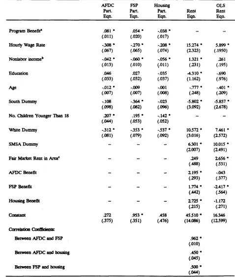
Table 1II.2 shows estimates of the full model, including the rent equation (ignoring, for the
moment, the last column). The coefficients on the variables in the participation equations are
generally of the same sign and significance as reported in Table III.l, which should be the case since
there is no "feedback _from the rent equation to the participation equations in this simple model.
In the rent equation, rental expenditures are seen to be positively affected by the wage rate and
nonlabor income. Moreover, those expenditures are positively affected by the amount of program
benefits received from each of the three programs. The error terms in the participation equations
are positively correlated with each other, but are negatively correlated with the error term inthe rent
equation. All of the correlation coefficients are statistically significant. Thus, female heads with
higher rental expenditures are less likely to participate in these programs. 6
These last correlations are important because they are an indication of serf-selection bias. The
fact that they are significant implies that serf-selection bias is present. In addition, their negative
values indicate the direction of such bias. Specifically, they indicate that families with low rental
expenditures are more likely to participate in AFDC, FSP, and housing programs/ndependent of the
direct effects of benefits in those programs. Thus, the types of recipients in these programs are
"self-selected" by _ rent leve_. This suggests, in turn, that a simple comparison of rent levels of
6 Aa the table indicates, only one variable (number of children younger than 18) appears in the participation equation and not in the rent eapenditure equation. Preferably, there should be three such variables, one for each equation. In addition, it is certainly possible that this particular variable has direct effects on rental expenditure, in which case adifferent type of variable should be used. One category of variables that might be appropriate is that which consisting of variables that affect the 'cmts' of participation, such as the 'access' variable we mentioned previously in the report. Unfortunately, our data set contains no direct measures of acce_ or other cost.
TABLE Ill.2
RESULTS OF THE ESTIMATION: THREE PARTICIPATION EQUATIONS AND RENT EQUATION
AFDC FSP Housing OLS
Part. Part. Part. Rent Rent
Eqn. Eqn. F.qn. Eqn. Eqn.
Program Benefit a .081 * .054 * -.038 * -
-(.011) (.020) (.017)
Hourly Wage Rate -.308 * -.270* -.208* 15.274* 5.899 *
(.067) (.065) (.074) (2.323) (.1950)
Nonlabor incomeb -.042 * -.060 * -.056* 1.321 * .261 (.013) (.010) (.011) (.231) (.195) Education .046 .027 -.035 -4.310 * -.690
(.033) (.032) (.037) (1.162) (.976)
Age -.012* -.009 -.001 -.777 * -.401* (.007) (.007) (.008) (.248) (.209)
South Dummy -.108 -.364 * -.023 -5.802* -5.837 *
(.098) (.082) (.096) (3.092) (2.678)
No. Children Younger Than 18 .207 * .195* -.142* -
-(.044) (.053) (.O52)
White Dummy -.312* -.353 * -.537 * 10_572 * 7.461 * (.081) (.079) (.092) (3.016) (2.572)
SMSA Dummy - - - 6.301 * 10.015*
(2.007) (2.491)
Fair Market Rent in Area c - - - .249 2.656 *
(.488) (.531)
AFDC Benefit - - - 2.195 * -.043
(.293) (.377)
FSP Benefit - - - 1.774 * -2.417*
(.442) (.564)
Housing Benefit - - - 2.725 * -1.172
(.215) (.271) Comtaat .272 .953 * .458 45.510 * 16346
(375) (351) (.476) (14.086) (12.599) Oxrelation Coeffgients:
Between AFDC and FSP .962 *
(.OLO)
Between AFDC and housing .450 *
(.045)
Between FSPand housing .500 *
(.044)
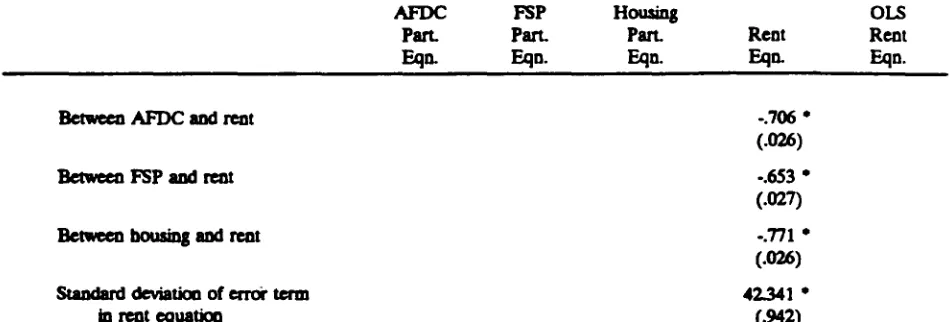
[image:18.610.72.550.143.707.2]TABLE 111.2(continued)
AFDC FSP Housing OLS
Part. Pan. Pan. Rent Rent
Fan. _n. Eqn. Fan. _n.
Between AFDC andrent -.706*
(.0-26)
Between FSP and rent -.653*
(.027)
Between housing and rent -.771*
(.026)
Standard deviation of error term 42.341 *
in rent equation (.942)
NOTE Standarderrors in parentheses.
·Weekly. Measured atzero hours of work. Coefficient is multiplied by 10.
bWeekly. Coefficient is multiplied by10.
eCoeffgient ismultiplied by10.
OLS = ordinary least squares.
·StaUgically significantat the 90 percent level
..e.
participants and nonparticipants is likely to show lower rent levels for participants, which might be
mistakenly interpreted as a negative effect Of participation on rental expenditures.
This suggestion isconfirmed by the last column in Table III.2, which shows ordinary least squares
regression estimates of the rent equation without any control for serf-selection bias. The coefficients
on aH three benefit levels are in this case negative, and one of these coefficients is statistically
si?iflcant. As a result, misleading conclusions would have been drawn from such estimates of the
rent equation.
Table 1II.3 shows the run times for various models and provides evidence that it is
computationally feasible to estimate these models using modern computers. The computer used for
the estimation was a mainframe Amdahl, close in capability to a standard IBM mainframe.
Microcomputers with 386 and 486 chips are somewhat slower than such mainframes but not so much
as to make the times shown in the table unrepresentative. The first two rows of the table show the
CPU minutes required for estimating the three participation equations only, but without any
independent variables-that is, only with intercepts. We did not present the results of these estimates
earlier because they are of no substantive interest; however, they do permit us to determine the effect
of the independent variables themselves on run times. As the table shows, the run time for the
intercept-only models was only 1.5 - 3.0 minutes, and the run time for the model consisting of the
three fully specified participation equations (that is, the model shown inTable IH.l) was much
more--16.8minutes. Therefore, the independent variables do indeed constitute most of the run time. When
the rent equatioa is added, the run time is about 30 minutes of CPU time. This run time is well
within the Capllb_ of most mainframes and most 386 and 486 micros as well.
The models estimated in Table IH.3 were estimated sequentially, starting with the model inthe
first row and then proceeding to the model in the next row. The "starting values" for each row were
obtained from the estimates obtained from the simpler model in the previous row. For this reason,
perhaps a more accurate estimate of the total run time for each model would be the sum of the run
TABLE m.3
RUN TIMES FOR'VARIOUS SPECIFICATIONS
OF THE MODEL
CPU Minutes Approx. Total Cumulative per Iteration CPU Minutes Run Time
Three Participation Equatiom Only
Intercepts only, no correlations 0.15 1.50 1.50
Intercepts only, correlations 0.24 3.00 4.50
Full specification, with correlations 0.85 16.80 21.30
Three Participation F.xluatiom plus Rent 1.20 28.80 50.10 Equation
NOTE: CPU times are for an Amdahl mainframe roughly equivalent in power andspeed to the IBM 3090 series.
times for that model and the previous ones. This is shown in the final column of the table as
cumulative run times. For the final model, this cumulative run time isabout 50 minutes. This is still
within computational feasibility. ?
Some experimentation was conducted on the number of "draws" required for estimation. The
results presented in Tables III. l-ITl.3 are for 20 draws, a number determined by starting at a Iow
number of draws and increasing that number until the estimates no longer "changed _with increasing
numbers of draws. Different models estimated on different data sets may require more or less
numbers of draws. We should note that the run time isroughly linear in the number of draws--that
is, a model requiring 40 drawswould require roughly double the CPU times shown inTable Ill.3, and
a model requiring 10 draws would require roughly haft the run times shown in the table.
Ge_raUzability to Other Applications. The example we have illustrated here involves only
three programs, and it involves a particular population group (female heads) and three particular
programs (AFDC, Food Stamps, and public housing). Practical issues may arise when extending the
technique to other applications.
One issue that might arise in other applications isthe distribution of the sample across different
program categories. In our SIPP data, a significant fraction of the sample participates ineach of the
three programs (30 percent in AFDC, 40 percent in FSP, and 17percent in housing). Application
of the technique to sets of programs where the sample is "thin _ for some programs (e.g., !ess than 5
percent) may make estimation difficult. For example, studies of multiple program participation among
husband-wife couples often suffer from small sample-size problems because there aresome programs
(e.g, AFDC-UP) for which their participation rates are quite small.
This problem is not unique to our estimating technique, for it arises in any participation study.
However, it ismore likely to arise here because multiple programs areconsidered and hence at least
? Each of the individual run time entries in the table is itself a sum of separate runs, each of which tried a set of "trial values" of all the coefficients, as described in the last section. Thus those
one of them may have a Iow participation rate. In addition, because our technique involves the
estimation of the correlation of program participation, it implicitly requires sufficient numbers of
households to participate in some combination of programs. This requirement may be difficult to
meet in small samples.
A second issue of generalizability relates to the extension of the model to four programs. First
of all, the run times given above are not linear with respect tothe number of programs involved. We
have illustrated only three programs, but the software we provide is capable of accommodating from
one to four programs. Each additional program participation equation increases the run time more
than proportionately because additional correlations and form_s of self-selection bias must be
estimated. In addition, the small sample size problem mentioned previously may make estimation
with four programs difficult. If, for example, multiple program participation among AFDC, FSP,
W]C, and either SBP or NSLP were considered, it is possible that samples might be quite small for
some of the programs and some of the combinations.
Finally, we might note that the variable used as the dependent variable in the "outcome"
equation does not affect the run times. Hence, using food expenditures instead of rent, for example,
should have no effect on these computational results.
IV. SUMMARY
In this report we described a new method for handling the problem of serf-selection bias in the
context of estimating the effects of a single assistance program when there is multiple program
participation. We also summarized the results of applying this program. The new method was
applied to the SIPP, and a four-equation model consisting of three participation equations and one
outcome equation was suc,cessfuHy estimated. The computational burden of the estimation ismore
than that associated with ordinary methods, but it is still well within the power of modern mainframes
and high-powered microcomputers. The evidence we report istherefore favorable, and the technique
appears to be suitable for application to problems involving self-selection bias for FSP recipients. We
note that application of self-selection adjustment methods in general, as well as our method, requires
the data set to contain variables that affect program participation but which do not directly affect the
outcome variable of interest. We recommend that when data containing such variables but containing
information on food expenditures or diet quality become available, program effects on those
outcomes to be estimated with our proposed technique.
At the time of this writing, the data set most likely to be useful for these techniques isthe
1989-91 CSFII, which has information on household food expenditures and individual food intake. The
CSFII has appro_fimately 1600 households in the Iow-income sample and 3500 in the population
sample, which should be enough to generate sufficient numbers of observations in the major programs
(FSP, AFDC, _ perhaps WIC, SBP, and NSLP) with which FNS isconcerned. The sample size
may not be lnrl_ enough to permit estimation of four separate participation equations (i.e., four
programs), however, an issue we disc_ previously. Another poss_le data set isthe 1996 survey
of food use currently under discussion, which will have information on household food use on a
low-income sample of approximately 5000 households.
REFERENCES
Devaney, B., and R. Moffitt. "Dietary Effects of the Food Stamp Program." American Journal of Agricultural Economics, February 1991, pp. 202-211.
Fraker, T., S.K. Long, and C.E Post. "Assessing Dietary Adequacy and Estimating Program Effects: An Application of Two New Methodologies Using FNS's Four-Day File for the 1985 CSFII." Washington, DC: Mathematica Policy Research, 1989.
Fraker, T., and R. Moffitt. "The Effect of Food Stamps on Labor Supply: A Bivafiate Selection Model." loumal of Public Economics, vol. 35, 1988, pp. 25-56.
"The Effect of Food Stamps on the Labor Supply of Unmarried Adults without Dependent Children." Washington, DC: Mathematica Policy Research, 1989.
Heckman, J.J. "Sample Selection Bias as a Specification Error." Econometrica, vol. 47, January 1979, pp. 153-161.
Keane, M. "A ComputationaUy Practical Simulation Estimator for Panel Data." Mimeographed, University of Minnesota, 1990.
Keane, M., and R. Moffitt. "A Structural Model of Multiple Welfare Program Participation and Labor Supply." Mimeographed, University of Minneaota, 1991.
Long, S.K. _rhe Impact of the School Nutrition Programs on Household Food Expenditures." Washington, DC: Mathematica Policy Research, 1988.
McFadden, D. "A Method of Simulated Moments for Estimation of Discrete Response Models without Numerical Integration." Econometrica, vol. 57, September 1989, pp. 995-1026.
Maddala, (}.S. Limited-Dependent and Qualitative Methods in Economem'cs. New York: Cambridge University Press, 1983.
Pakes, A., and D. Pollard. "Simulation and the Asymptotics of Optimization Estimators."
Econometrica, vol 57, September 1989, pp. 1027-1057.
Contract No.: 53-3198-9-31 MPR Reference No.: 7890-009
SOFTWARE DOCUMENTATION FOR PROGRAMS TO ESTIMATE
SELF-SELECTION MODELS WITH MULTIPLE EQUATIONS USING
THE METHOD OF SIMULATION
December 3, 1992
Supplement to Report Entitled:
'THE ESTIMATION OF FOOD STAMP SELF-SELECTION MODELS USING
THE METHOD OF SIMULATION"
Authors:
Michael Keane University of Minnesota
Robert Moffitt
Brown University
Submitted to: Submitted by:.
U.S. Department of Agriculture Mathematica Policy Research, Inc. Food and Nutrition Service 600 Maryland Avenue, S.W.
3101 Park Center Drive Suite 550
Alexandria, Virginia 22302 Washington, D.C. 20024
CONTENTS
Chapter Page
I INTRODUCTION ...1
II FILES USED IN ESTIMATION... 2
HI INA.DAT AND INB.DAT ... 4
IV REMARKS ON USAGE ... 7
REFERENCES ... 10
APPENDIX A: STATISTICAL MODELS AND ESTIMATION
METHOD ... · ... 11
APPENDIX B: STRUCTURE OF THE FORTRAN PROGRAMS ... 14
I. INTRODUCTION
This document provides instructions for the use of the programs SIMA. FOR and SIMB.FOR
to estimate models of multiple welfare program participation, with or without an extra equation for
an outcome variable. This document and the two programs are provided as supplements tothe final
report to FNS entitled "The Estimation of Food Stamp Self-Selection Models Using the Method of
Simulation _ by Michael Keane and Robert Moffitt (1992), submitted by Mathematica Policy Research.
That report should be read prior to reading this document.
The statistical models estimable with the programs SIMA. FOR: and SIMB.FOR are documented
in detail in Appendix A of this report. They are also presented in the aforementioned final report
to FNS. The model in SIMA. FOR consists of up to four welfare program participation equations. _
Each equation can have different independent variables. The model in SIMB.FOR permits the
addition of an outcome equation with a continuous dependent variable (e.g., food expenditures or
some other variable that may be affected by program participation). That equation can contain
regreasors that do or do not overlap with those in the participation equations. In FNS applications,
this equation willoften contain the program benefit(s) and/or program participation dummy variables.
The error terms in the participation equations, and in the extra outcome equation ff added, are
assumed to be distributed according to a multivariate normal distribution with an unrestricted
covariance matrix. If the extra outcome equation is added, this implies that the program fully
accounts for the correlations that induce selection bias in that equation.
The program._ employ the method of simulated moments (MSM) to estimate the models, z
I If additional programs are needed, the program can be adapted for that purpose. A number of the matrices in the Fortran program would have to be increased in dimension.