Combining geographical information systems and input output models: concept and initial ideas

Combining geographical information

systems and input-output models:

concept and initial ideas

Guilhoto, Joaquim José Martins and Hewings, Geoffrey J.D.

and Takashiba, Eliza H. and Silva, Lana M.S da

Universidade de São Paulo, University of Illinois

2003

Joaquim J.M. Guilhoto1, Geoffrey J.D. Hewings2, Eliza H. Takashiba 3, Lana M.S. da Silva 4

Paper Presented at the

50

North American Meetings of the

Regional Science Association International

Philadelphia, Pennsylvania

November 20-22, 2003

PRELIMINARY VERSION

ABSTRACT

Since the initial input-output (i-o) models conceived by Leontief in the 1930’s, the input -output theory has gone through a lot of development at the theoretical as well as applied point of view. However, despite all the progress, there are two points that need further consideration into the analysis, one is with respect to an easy visualization of the information contained in an i-o system and another is related to the spatial dimension of the data. We do not mean that these topics have not been dealt with before, but, here both are combined in a single analysis where the Geographical Information Systems (GIS) are use to map and to visualize the i-o models. The data used to illustrate the initial concepts is based in the interregional i-o matrix constructed for six macro regions (Northeast, North, Central West, São Paulo, Rest of the Southeast, and South) of the Brazilian economy for the year of 1999 by Guilhoto et al (2003). The initial applications and analysis are done: a) with the i-o matrix in value terms; and b) with an estimation of impacts on total production, giving changes in the final demand of the households. However, new windows of analysis are open as this information can be combined with models of transportation, spatial data analysis, etc.

1

Department of Economics, University of São Paulo, Brazil; REAL, University of Illinois; and CNPq Scholar. This author would like to acknowledge the grant received from the Hewlett Foundation through the Center for Latin American and Caribbean Studies at the University of Illinois. E-mail: [email protected].

2

Regional Economics Applications Laboratory (REAL), University of Illinois (USA). E-mail: [email protected]. 3

ESALQ, University of São Paulo (USP). E-mail: [email protected] 4

1. Introduction

Since the initial input-output (i-o) models conceived by Leontief in the 1930’s, the input -output theory has gone through a lot of development at the theoretical as well as applied point of view. However, despite all the progress, there are two points that need further consideration into the analysis, one is with respect to an easy visualization of the information contained in an i-o system and another is related to the spatial dimension of the data. We do not mean that these topics have not been dealt with before, but, here both are combined in a single analysis where the Geographical Information Systems (GIS) are use to map and to visualize the i-o models. The data used to illustrate the initial concepts is based in the interregional i-o matrix constructed for six macro regions (Northeast, North, Central West, São Paulo, Rest of the Southeast, and South) of the Brazilian economy for the year of 1999 by Guilhoto et al (2003). The initial applications and analysis are done: a) with the i-o matrix in value terms; and b) with an estimation of impacts on total production, giving changes in the final demand of the households.

The next section will present the basics input-output models, while section 3 does the same for geographical information systems. Section 4 presents a brief overview of the Brazilian economy and the six macro regions considered in the analysis. Section 5 presents the GIS maps derived from the combination of both methodologies, and the final comments are made in section 6.

2. Input-Output Models

Inter-industries flows in a specific economy are determined by technological and economic factors, and these flows can be described by a system of simultaneous equations represented by:

X  AXY (1)

In the model above, the final demand vector is usually considered exogenous to the system; thus, the total production vector is determined only by the final demand vector, that is:

X BY ₍₂₎

and

B 

b g

where B (n x n) is the Leontief inverse matrix.

Starting from equation (3), we can evaluate the impact of different changes in the final demand on the total production, import volumes, total salaries, etc. Thus, for example,

X B Y

   (4)

ˆ

M m X

   (5)

ˆ

W w X

   (6)

where Y , X, M and W are (n x 1) vectors which show respectively the final demand increase, and the impacts on total production, on imports and total wages; mˆ and wˆ are diagonal

(n x n) matrices in which the main diagonal elements are the coefficients of import and salary, respectively.

For the case of the interregional system, the above idea repeats itself, however there is a change in the matrix structure, where now, for the 2 regions case, the A, X and Y matrices are now given by

A A A

A A LL LM ML MM              (7) X X X L M         

 (8)

Y Y Y L M         

 (9)





X  IA  Y (10)

where the interregional dimension is now being taken into consideration (Miller & Blair, 1985).

3. Geographical Information System Models

Geographic Information System (GIS) is the term applied for systems that carry the computational treatment of geographic data and retrieve information not only alphanumeric characteristics, but also through its geographical localization.

So that is possible, the geometry and the attributes of the data in a GIS must be georreferenced, located in the terrestrial surface and represented in a cartographic projection. The requirement to store the geometry of geographic objects and its attributes represents the basic principle for GIS’s. For each geographic object, the GIS needs to store its attributes and the some graphical representations associates. There are three great ways to use a GIS a) as tool for production of maps; b) as support for space analysis of phenomena; and c) as a geographic data base, with functions of storage and recovery of space information. To clarify more the subject, some definitions of GIS are related in Burrough and McDonnell (1998).

The GIS definitions reflect, the multiplicity of uses and possible views of this technology and point a perspective to interdisciplinar use. Moreover these concepts, the main characteristics of GIS are: a) to insert and to integrate geographical information, proceeding in database from cartographic, urban and agricultural cadastre, images of satellite, numerical land nets and models; and b) offer mechanisms to combine some information, through algorithms of manipulation and analysis, as well as consulting, retrieving, to visualize and to locate the content of a georreferenced database.

of the ground. When a map contains information about an only object or subject, it is called thematic map. And, when the variation in the attributes of the object is represented in classes and, each class is represented by different colors, these maps are named chorochromatic maps.

In general, the more used form to represent entities in a space-time context is through maps. In GIS the elements of a map are stored of georeferenced form according to a coordinate

reference system. The GIS’s originally had been developed for natural resources quantification, in view of the planning use of these resources. The use of this tool for other sciences has occurred quickly, being its application in environment, management and socio-economic studies. In socio-economic applications, the GIS are used for planning and changes evaluation in a region with determined politics. Câmara et al. (1996) describes, within socio-economic applications, the following groups: a) land use cadastre; b) agroindustry and irrigation; c) human occupation; d) urban and regional cadastres; e) public utilities, i.e., gas, electricity, telephone lines, sewerage systems; and e) economic activities grouping marketing and industries. The data used in socio-economic applications, frequently are gotten through tax collections, digitized urban maps and air photographs.

4. A Brief Overview of the Brazilian Regions

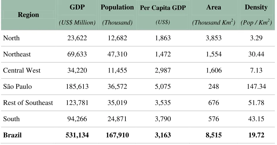
Information for the 6 six macro Brazilian regions being considered here can be seen in table 1, and figure 1. The Brazilian economy presented a GDP of around US$ 531 billion in 1999, with a population of around 168 million people, which gives a per capita GDP of US$ 3,163. And giving the area of 8,515 thousand km2, de density of the population is of 19.72 persons per km2.

The most developed regions in Brazil are the Southeast (São Paulo and Rest of the Southeat) and the South region. In the Southeast region, São Paulo has a share of 34.95% of the Brazilian GDP with 21.78% of its population and 2.92% of the territory, with the highest per capita income of all regions. The Rest of Southeast, with 7.94% of the territory, and 23.31% of the GDP and 20.86% of the population, is the third highest per-capita income of all the regions being considered here.

The South region has a share of 17.75% in the Brazilian GDP with 6.77% of the territory and 14.81% of the population. São Paulo is the most industrialized region in Brazil, while the South region is the one more closed to the Mercosur countries, which is the region that due to the continental size of Brazil could be the one to get the most benefits from the Mercosur integration. The Central West region has been an important region for Brazil in terms of agriculture, mainly because of the favorable type of land that this region has, and it has a reflex in its share in the population (6.82%) and GDP (6.44%) of Brazil.

Table 1. Main Indicators of the Brazilian Regions, Considered in the Model, for 1999 Region GDP (US$ Million) Population (Thousand)

Per Capita GDP

(US$)

Area

(Thousand Km2)

Density

(Pop / Km2)

North 23,622 12,682 1,863 3,853 3.29

Northeast 69,633 47,310 1,472 1,554 30.44

Central West 34,220 11,455 2,987 1,606 7.13

São Paulo 185,613 36,572 5,075 248 147.34

Rest of Southeast 123,781 35,019 3,535 676 51.78

South 94,266 24,871 3,790 576 43.15

Brazil 531,134 167,910 3,163 8,515 19.72

5

. A GIS

–

IO Model for the Brazilian Economy

In this section it will be presented the results of implement the GIS-IO model for the Brazilian economy.

The basic idea in implementing the model is to have the two models running together, with the IO model running in the background and the GIS model showing the results in the map. The results showing here are a first attempt to combine these models, and should be viewed as so. As times develop and ones get more acquainted with the process new approaches and application certainly will be developed.

As so, this section is divided into three parts, in the first one the basic IO data base is presented, the second one presents the implementation of the GIS model, while in the third one the results of an application made for the Brazilian economy is presented.

5.1. IO Data Base

The IO data base for the model consists of an interregional system constructed for the Brazilian region, for six macro regions (presented above), for 90 sectors, for the year of 1999, by Guilhoto et al. (2003).

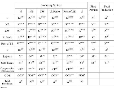
To implement the system, the number of sectors were aggregated to 25, in a schematic way the overall system can be seen in figure 2 below.

The first set of the GIS maps (Figures 4 to 11) were constructed using the values of the matrix, with different layers, where each layers can be seen as a row in the schematic matrix of figure 2.

Figure 2: Schematic Representation of the I-O System Used in the Model

Producing Sectors _Final Demand

Total Production N NE CW S. Paulo Rest of SE S

N ICN N ICN NE ICN CW ICN SP ICN RSE ICS S YN XN

NE ICNE N ICNE NE ICNE CW ICNE SP ICNE RSE ICNE S YNE XNE

CW ICCW N ICCW NE ICCW CW ICCW SP ICCW RSE ICCW S YCW XCW

S. Paulo ICSP N ICSP NE ICSP CW ICSP SP ICSP RSE ICSP S YSP XSP

Rest of SE ICRSE N ICRSE NE ICRSE CW ICRSE SP ICRSE RSE ICRSE S YRSE XRSE

S ICS N ICS NE ICS CW ICS SP ICS RSE ICS S YS XS

Imports MN MNE MCW MSP MRSE MS MY MX

Sale Taxes STN STNE STCW STSP STRSE STS STY STX

Compensation of Employees CE

N

CENE CECW CESP CERSE CES

GOS GOSN GOSNE GOSCW GOSSP GOSRSE GOSS

Total

Production X

N

XNE XCW XSP XRSE XS

Where:

GOS – Gross Operating Surplus IC – Intermediate Consumption

5.2. GIS - Digital Elevation Modeling

One layer with the six macro regions limits was generated as a result of the digitized base map overlaid.

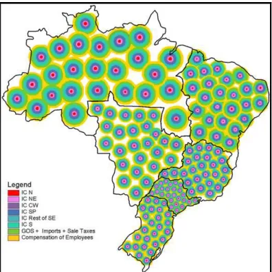
Eight layers were created to represent the economic variables, considered in this study (Figure 3): a) compensation of employees; b) sale taxes, plus imports, plus gross operating surplus; c) intermediate consumption north region; d) intermediate consumption northeast region; e) intermediate consumption central west region; f) intermediate consumption São Paulo region; g) intermediate consumption rest of southeast region; and h) intermediate consumption south region. In each layer, 25 circles were digitized to represent the 25 sectors of the interregional i-o system for the six macro regions. Finally, economic values were attributed to each circle in each layer.

The circles did not cover the domain of interest completely, for this reason, interpolation was necessary to the conversion of datasets points to represent a continuous surface (Figure 3).

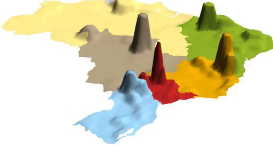
Continuous surface are represented by regular grid, in this case, each economic variable is represented by a separate overlay and each grid cell is allowed to take a different value to generate a DEM, where the elevation data is a monetary value.

The shaded relief grid was created with sun azimuth of 350°and an altitude of 45° to cast a shadow over the DEM area. An image results with topographic relief appropriately highlighted.5

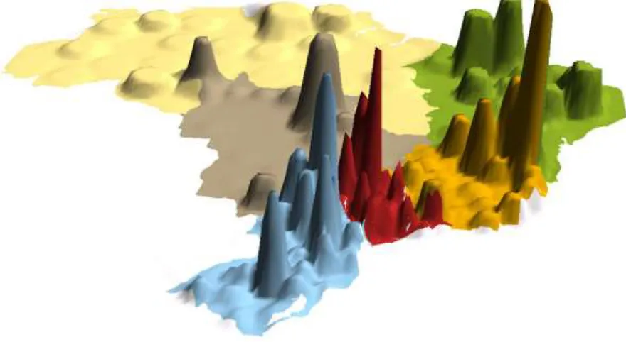
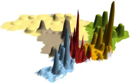
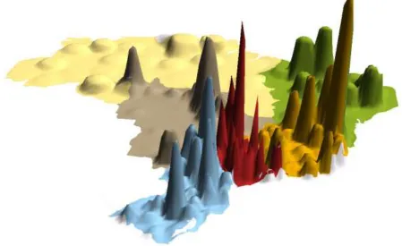
5.3. Results for the GIS – IO Model

The results for the GIS – IO model are presented into two parts, in the first one the results shows how the value of total production by sector, in each region, is breaking down into its components, i.e., gross operating surplus, compensation of employees and intermediate consumption from each one of the macro regions. In the second one it is measured the impact that one unit of a standard household consumption will have in the sectoral total production in each one of the regions being considered in the analysis.

5

Figure 3: GIS-IO Map, 2 Dimensions Level

5.3.1. Decomposition of the Total Production Value

From Figures 4 to 11 the value of total production in each sector, and in each region, is decomposed by its components.

In Figure 4 it can be seen that the highest shares of the compensation of the employees are concentrated into few sectors and regions, mainly the regions of São Paulo, Rest of Southeast and South.

When the gross operating surplus, the imports, and the sales taxes are added to the system (Figure 5) one can see that the shape of the landscape becomes close to the final shape (Figure 11), showing the importance of these values, together with the compensation of employees, in determining the value of the total production in the economy, and the structure of total production distribution among the sectors and regions.

Figure 4: GIS-IO Map, Layer 1 = Compensation of Employees

Figure 5: GIS-IO Map, Layer 2 = L1 + GOS + Imports + Sale Taxes

Figure 6: GIS-IO Map, Layer 3 = C2 + IC South

Figure 7: GIS-IO Map, Layer 4 = C3 + IC Rest of SE

Figure 8: GIS-IO Map, Layer 5 = C4 + IC SP

Figure 9: GIS-IO Map, Layer 6 = C5 + IC CW

Figure 10: GIS-IO Map, Layer 7 = C6 + IC NE

Figure 11: GIS-IO Map, Layer 8 = C7 + IC North

5.3.2. Impacts of a Standard Household Demand in Each Region

Figures 12 to 17 show how the impact of standard unit of consumption in each one the regions will have in the origin region and in the other regions being considered here.

It can be seen that the three most integrated regions are the most developed ones, i.e., São Paulo, rest of the southeast, and south. These are the regions that receive the most of the interregional impacts, and among them, São Paulo is the one that receives most of the impacts.

Figure 12: GIS-IO Map, Impact of household consumption - North

Figure 13: GIS-IO Map, Impact of household consumption - NE

Figure 14: GIS-IO Map, Impact of household consumption - CW

Figure 15: GIS-IO Map, Impact of household consumption - SP

Figure 16: GIS-IO Map, Impact of household consumption – Rest of SE

Figure 17: GIS-IO Map, Impact of household consumption - S

6. Final Comments

The work present here was just a first attempt to combine GIS and IO system such that it should be possible in the future, among other things: a) to have a better understanding of how the economy works; b) to better visualize the I-O data; c) to have a tool that can be used by business men and policy makers to analyze and to visualize the possible impacts of their decisions in their region and the other regions being considered in the analysis, by just clicking a bottom; d) to combine other variables into the analyzes, like employment, energy use, pollution generation, transportation system, income, etc.; and e) to use this system with other tools of analysis, statistical and mathematical.

However, a close look of the model draws attention for some aspects that needed to be better worked.

The sectors displayed here are correctly located in a given region, but their location inside a given region do not correspond to the real geographical position. It happens here because, on one hand, sometimes it is not know the correct location of the sector, on the other hand, the sector is located in different points of a given region.

The size of the “mountains” base is adjusted to the size of the regions, and this has an impact in the visualization of the system.

On implementing the model in a real world one has also to be faced with the problem that different locations of a same sector will occur on the system. Probably each location has to be treated as a different sector, but this will increase the size and complexity of the model, generating an increasing demand on data and computational resources.

Rerefences

Burrough, P.A. and R.A. McDonnel (1988). Principles of Geographical Information Systems. New York : Oxford University Press, 1998. 333 p.

Câmara, G., M.A. Casanova, A.S. Hemerly, G.C. Magalhães, and C.M.B. MEDEIROS (1996).

Anatomia de Sistemas de Informação Geográfica. Campinas: Instituto de Computação, 1996. 193p.

Guilhoto, J.J.M. et al. (2003). “Interregional Input-Output Systems for the Brazilian Economy in

1999”. Work in Progress. Department of Economics, FEA, University of São Paulo.

IBGE (2002a). Contas Regionais do Brasil, 1985-2000. Rio de Janeiro.

IBGE (2002b). Brasil em Números 2002. Rio de Janeiro. Vol. 10.

Leontief, W. (1951). The Structure of the American Economy. Second Enlarged Edition. New York: Oxford University Press.