Wind Characteristics Analysis for Selected Site
in Algeria
Maouedj Rachid
Unity of Research in Renewable Energies inSaharan Medium. Adrar. Algeria.
Diaf Said
Centre of Renewable Energies Development, B.P 62, Bouzareah, Algiers, Algeria l
Benyoucef Boumediene
Unity of Research in Materialsand Renewable Energies, University of Tlemcen, Algeria
ABSTRACT
The wind characteristics of four locations in Algeria (Algiers, Oran, Adrar and Ghardaia) have been assessed. The data were collected over a period of 13 year. The wind speed characteristics and wind power potential of each station have been determined using Weibull distribution.
The annual average wind speed for the selected sites ranged from 3.81 m/s to 6.38 m/s and a mean wind power density from 97.26 w/m2 to 270.17 w/m2 at standard height of 10 m. The wind data at heights 30 m and 50 m were obtained by extrapolation of the 10 m data using the Power Law.
Power estimates use four configurations of the General Electric GE 1.5-MW series turbines that varied in rotor diameters, cut-in, cut-out and rated speeds.
Keywords
Wind speed; wind energy; Weibull parameters; wind generators; capacity factor.
1.
INTRODUCTION
Since 2010, Algeria is implementing an ambitious strategy for encouraging and developing renewable energy in its territory. This strategy would gradually replace the use of gas, which currently is the only resource for the country's electricity generation by other energy sources like solar, wind and nuclear energy [1].
National policy for the renewable energies promotion and development is governed by laws and regulations adopted over recent years (law on energy conservation, law on the promotion of renewable energy within a framework of sustainable development, law on electricity with its accompanying decree on the diversification costs) reveal the will of the state to make these energies, the future energies for the country, by encouraging a greater contribution to the national energy mix, and also this policy relies on a whole network of organisations and business companies within of higher education and scientific research and the ministry of energy and mines each one dealing with the development of renewable energies [1,2].
Algeria has a considerable wind resource, whose potential is especially significant in the south with average speeds of 4 to 6 m / s, is also a valuable resource that can supply domestic needs in remote sites, while the north is found to be less windy with the exception of microclimates in the coastal region of Oran, Bejaia and regions of Tiaret, Biskra and Setif [1,3].
The aim of this paper present a study of the statistical properties of the wind speed and wind potential in Algeria by considering four locations in which the data are recorded by Algerian Meteorological National Office (MNO), and
presentation of a simple method for determination of pairing between sites and wind generators.
2.
GEOGRAPHICAL SITUATION OF
ALGERIA
Algeria is located in North Africa bordered in north by the Mediterranean Sea (1200 km), in the east by Tunisia (965 km) and Libya (982 km), in south-east by Niger (956 km,), in south-west by Mali (1,376 km) and Mauritania (463 km), in west by Morocco (1,559 km) and the Western Sahara (42 km). Its geographical coordinates are represented by latitude of 28º 00´North of the equator and longitude of 3º 00´ East of Greenwich [4].
Algeria is the largest country in Africa, in the Arab world, and the Mediterranean and is classified the eleventh in the word in term of its land area. It occupies an area of 2,400,000 km2, with an estimated population of 37.1 million as of 2012 and a population density at 16,08 inhabitants/km2 [5].
3.
WIND DATA
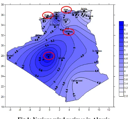
The geographical locations (latitude, longitude and altitude) for the sites considered in this study are presented in Table 1 and Fig.1. Wind data for 20 meteorological stations were obtained from the Algerian MNO. The data were collected over a period spanned between 1976 and 1988 [6, 7].
At all stations the measurements are obtained at a height of 10 m above sea level.
Therefore, the wind parameters are extrapolated from the standard height of 10 m to 30 m and 50 m using the power low expression. The Weibull parameters k and c are determined and used to estimate the annual mean wind speed and the wind power density for each site.
Table 1 and Fig. 1 shows the geographical location of the study area [8-9].
Table 1. Geographical location for the different sites
Sites Longitude (°)
Latitude (°)
Altitude (m)
Topographic Situation Algiers
Oran
03° 15’ E 00°37’ W
36° 43’N 35° 38’N 25 99
Coastal zone
Adrar Ghardaia
00°17’ W 03° 49’ E
27° 53’N 32° 23’N 264 450
Fig 1: Various wind regimes in Algeria
4. MATHEMATICAL FORMULATION
4.1. Weibull method
The Weibull distribution function [10, 11] is the most frequently used model to describe the distribution of the wind speed. This function gives a good match with the experimental data. It is characterised by two parameters k and c. this distribution takes the form
k kc
v
c
v
c
k
V
f
exp
1for (k>0,V>0,c>1) (1)
Where v is the wind speed, k is the dimensionless shape parameter, describing the dispersion of the data and c Weibull scale parameter in the unit of wind speed (m/s).
Moreover, the cumulative density function of the Weibull distribution is defined as [10, 11]
01
).
(
)
(
k C Ve
dv
V
f
V
F
(2)The mean of the distribution [10, 11], i. e., the mean wind speed, Vm is equal to
k
c
dv
V
f
V
m1
1
0 (3)The most probable wind speed (VE), which represents the most frequent wind speed, is expressed by [12]:
k E
k
c
V
12
1
.
(4)Wind speed carrying maximum wind energy can be expressed as follows [12]:
k F
k
c
V
11
1
(5)The variance 2 of the data is then defined as [13, 14]
k
k
c
dv
V
f
V
V
)
1
2
1
1
(
2 20
2
(6)The standard deviation is then defined as the square root of the variance [14].
Variance
deviation
Stadard
(7)The average cubic speed of the wind is given by the following relation [15]
k
c
dv
V
P
V
V
31
3
0 3 3
(8)
Where is the defined gamma function, for any reality x positive not null, by
x
t
t
x
dt
10
exp
withx
0
(9)4.2. Vertical extrapolation of wind speed
The wind data measurements used in this study are used from stations set at a standard height of 10 m. The vertical extrapolation of wind speed is based on the Power law [16-18]
ref refz
z
z
v
z
v
(
)
(
).
(16)Where v (zref) is the actual wind speed recorded at height zref, v (z) is the wind speed at the required or extrapolated height z and α is the surface roughness exponent is also a terrain-dependent parameter.
4.3. Vertical extrapolation of Weibull
parameters:
The Weibull parameters are also function of height [18-20],
n ref ref
z
z
z
c
z
c
(
).
)
(
(17)
10
.
088
.
0
1
10
.
088
.
0
1
).
(
)
(
z
Ln
z
Ln
z
k
z
k
refref (18)
n is a scalar which can be obtained by the relation
n is a scalar obtained using the relation
10
.
088
.
0
1
))
(
(
.
088
.
0
37
.
0
ref refz
Ln
z
c
Ln
4.4. Estimating wind power
The kinetic energy of air stream with mass (m) and moving with a velocity (v) is given by [21]
2
2
1
mv
E
[J] (20)The power in moving air is the flow rate of kinetic energy per second. Therefore [21]:
t
v
m
t
E
P
2.
.
2
/
1
[w] (21)The wind power density (Pd) representing the power per unit area can be written [22]:
3 0
.
.
2
1
v
A
P
P
d
[w/ m2] (22)ρ0 is the standard air density, (1.225 kg/m3 )
A is the area swept by the rotor blades (A= .R2), [m2]
v is the mean wind speed, m/s
The theoretical maximum power that can be extracted from a wind turbine is limited by Betz’s law [23, 24]:
3 0
.
)
,
(
.
2
1
v
A
C
P
ext
p
(23)Cp (, β) the power coefficient, represents the wind turbine aerodynamic efficiency. It depends on the tip speed ratio and the blade pitch angle β. The theoretical maximum value for the power coefficient Cp_max is 0.59 (the Betz limit). The air density ρ0 varies with temperature and elevation. The monthly mean air density (kg/m3) is calculated using the equation [25]
T
Z
T
Z
T
,
)
353
.
049
.
exp
0
.
034
.
(
(24)Where
Z is the elevation of the site [m].
T is the monthly average air temperature [K]
Finally, the corrected wind power density (k.W.h/m2), can be computed using: 3
.
.
586
.
2
v
E
wdp
(25)According to [26-29], the wind turbine power curve can be well approximated with the parabolic law:
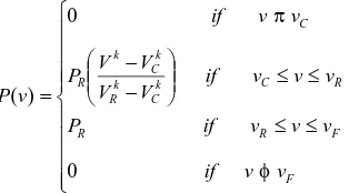
F F R R R C k C k R k C k R C v v if v v v if P v v v if V V V V P v v if v P 0 0 ) ( (26)
PR is the rated electrical power; vC is the cut-in wind speed,
vR is the rated wind speed, vF is the furling wind speed,
k is the Weibull shape parameter.
Integrating equation (26), this is [24, 30]:
0
(
).
(
).
(
).
(
).
F
c
v
v
avrg
P
v
f
v
dv
P
v
f
v
dv
P
(27)Substituting Eq.26 into Eq. 27 yields
R C F R v v v v R k C k R k C k Ravrg
f
v
dv
P
f
v
dv
v
v
v
v
P
P
.
.
(
).
.
(
).
(28)There are two distinct integration in Eq. 28 which to need be integrated. The integration can be accomplished by making the change in variable.
After calculate [24, 26, 31-33]
k F k R k C k R k C R avrg c v c v c v c v c v P P exp exp exp (29) avrg
P
can be expressed as:F R avrg
P
C
P
.
(30)
Where CF is the capacity factor.
5. RESULTS AND DISCUSSIONS
[image:3.595.300.558.502.567.2]The Weibull distribution parameters and characteristics speeds are evaluated, and the numerical results for four Algerians sites are presented in Tables 2 to 4.
Table 2. Weibull distribution parameters and characteristics speeds for different sites at 10 m height
Sites k (-)
c (m/s)
Vm (m/s)
<V3>
(m/s)3
[image:3.595.68.225.648.735.2](-) VE (m/s) VF (m/s) Algiers Oran Adrar Ghardaia 2.03 1.26 2.15 1.65 5.00 4.10 7.20 5.60 4.43 3.81 6.38 5.01 163.62 201.34 462.23 298.97 3.62 5.88 4.85 5.32 3.62 5.88 4.85 5.32 7.01 8.72 9.78 9.06
Table 3. Weibull distribution parameters and characteristics speeds for different sites at 30 m height
Sites k (-)
c (m/s)
Vm (m/s)
<V3>
(m/s)3
Table 4. Weibull distribution parameters and characteristics speeds for different sites at 50 m height
The wind speed data for the four selected station are presented in Fig.3. As shown, Adrar has the highest wind speed in the area, but present significant fluctuations between months and seasons. Ghardaia has also high wind speed with limited fluctuations over the year. Besides, Oran presents rather lower wind speed, while Algiers is the last windy site.
0 2 4 6 8 10 12
10 12 14 16 18 20 22 24 26 28 30 32 34 36
Me
a
n
t
e
mp
e
ra
tu
re
(
°C
)
Months Algiers
Oran Adrar Ghardaia
[image:4.595.327.525.231.669.2]Fig 2: Mean monthly temperatures for the selected sites.
0 2 4 6 8 10 12
3 4 5 6 7 8
Algiers Oran Adrar Ghardaia
Me
a
n
w
in
d
spe
e
d
s
(
m
/
s
)
Months
Fig 3: Mean monthly wind speeds for selected sites
[image:4.595.76.260.254.398.2]Fig 4: Weibull probability density function at 10 m height
Fig 5: Weibull cumulative distribution function at 10 m height
Fig 6: Monthly air density
Algiers Oran Adrar Ghardaia 1,11
1,12 1,13 1,14 1,15 1,16 1,17 1,18 1,19
Ann
u
a
l
a
ir
d
e
n
si
ty
(kg
/
m
3)
X Axis Title
Fig 7: Annual air density
It is noticed that the great decreases of the air density is recorded in the sites of Adrar and Ghardaia, these sites are respectively characterized by the very elevated heights above sea level (264 m and 450 m), while the weak variation is noticed in the very low heights sites, Algiers (25 m) and Oran sites (99 m).
The density of air decreases with the increase in site elevation and temperature as illustrated in Fig.6 and 7.
The highest decreases of the air density are found during the summer season in all stations and the lowest values are found during the winter season.
Sites k (-)
c (m/s)
Vm (m/s)
<V3>
(m/s)3
(-) VE
(m/s) VF
(m/s)
Algiers Oran Adrar Ghardaia
2.36 1.47 2.50 1.92
7.21 6.08 9.86 7.94
6.39 5.50 8.75 7.04
429.89 466.92 1056.17
695.98 4.34 6.82 5.53 6.17
09.35 10.91 12.47 11.52
5.71 2.80
[image:4.595.81.258.433.561.2] [image:4.595.82.254.607.736.2] Annual values of corrected wind power are smallest that the uncorrected wind power (see Fig.8).
We notice that the shape and scale parameters increase as the height increases. At 10m height, the shape parameter k varied between 1.26 (Oran) and 2.15 (Adrar) while the scale parameter c varied between 4.10 m/s (Algiers) and 7.20 m/s (Adrar), and for 50m height, the shape parameter varied between 1.47 (Oran) and 2.50 (Adrar) while the scale parameter c varied between 6.08 m/s (Algiers) and 9.86 m/s (Adrar).
The highest values of annual mean wind power density are found in Adrar (P10 = 283.12 W/m2), where the lowest values of annual mean wind power density are found in Algiers (P10=100.22 W/m2).
Fig 8: distribution of wind power density over Algeria at 10 m height
Algiers Oran Adrar Ghardaia
0 50 100 150 200 250 300 350 400 450 500 550 600
650 P10
Pc
10
P30
Pc
30
Pi
50
Pci
50
Po
w
e
r
(
W
/
m
2 )
[image:5.595.322.539.70.224.2]Fig 9: Computations of the annual corrected and uncorrected wind power by Weibull distribution for different heights.
Fig 10: Correlation between monthly values of corrected Pc and uncorrected wind power P of the selected stations
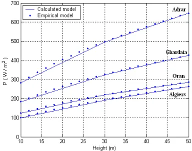
Fig 11: Correlation between monthly values of uncorrected wind power P and height Z of the selected stations.
[image:5.595.65.271.238.401.2] [image:5.595.332.524.270.421.2] [image:5.595.56.274.470.636.2] [image:5.595.332.522.502.653.2]Fig 13: Correlation between monthly values of uncorrected wind power P and wind speed V of the selected stations.
Fig 14: Correlation between monthly values of corrected wind power Pc and wind speed V of the selected stations.
A linear relation was observed between mean monthly power densities and measured mean monthly wind speeds. The correlation equation is (CC ≈ 0.997):
C
P
P
0
.
881
0
.
942
(31) [image:6.595.64.270.69.238.2]For the selected stations, a Correlation between monthly uncorrected wind power P and corrected wind power Pc with height Z has been investigated and illustrated in Fig.11 and Fig.12. A strong correlation has been found between P, Pc and Z, where we obtain a correlation coefficient of CC=0.99.
The recommended correlation equations are respectively given by:
b
Z
a
P
.
(32)b
C
a
Z
P
.
(33)Where a and b are constants, being dependent on the characteristics on the selected site, are provided respectively in Table 5 and 6.
The variation of monthly mean uncorrected power P and monthly mean corrected power PC with measured monthly mean wind speed are presented in Fig.13 and Fig.14. As can be seen, there are a strong correlation, CC>0.99, between the
monthly mean powers and the measured monthly mean wind speeds.
The recommended correlation equations are respectively given by:
b
V
a
P
.
(34)b
C
a
V
P
.
(35)Where a and b are constants, being dependent on the characteristics on the selected site, are provided respectively in Table 7 and 8.
Table 5. Parameters a, b and R2 of the empirical model of energy and for the selected stations.
Sites
a b
R2
Algiers
Oran Adrar
Ghardaïa
24.89588 37.09080 86.37732
54.50057 0.60249 0.52224 0.51441
0.52563 0.99991
0.99999 0.99996
[image:6.595.311.551.251.327.2]0.99999
Table 6. Parameters a, b and R2 of the empirical model of energy and for the selected stations.
Sites
a b
R2
Algiers
Oran Adrar
Ghardaïa
4.29842 7.09080
86.37730 54.50057
0.59983 0.52224 0.51441 0.52563
0.99989 0.99999 0.99996 0.99999
Table 7. Parameters a, b and R2 of the empirical model of energy and for the selected stations.
Sites
a b
R2
Algiers
Oran Adrar
Ghardaïa
1.96054 5.80200 2.20546 3.35429
2.64154 2.28701 2.61894
2.48265 0.99998 0.99996 0.99998
[image:6.595.70.265.297.447.2]1.00000
Table 8. Parameters a, b and R2 of the empirical model of energy and for the selected stations.
Sites
a b
R2
Algiers
Oran Adrar
Ghardaïa
1.93486 5.80200 2.20546 3.35429
2.62994 2.28701 2.61894
2.48265 0.99997 0.99996 0.99998
[image:6.595.308.553.382.458.2] [image:6.595.312.550.527.601.2] [image:6.595.311.550.659.734.2]Table 9 gives the technical specifications of four configurations of the General Electric (GE) 1.5-MW series wind turbine used in this study [34].
Table 9 . Characteristics of 1.5 MW Series Wind Turbine used in this study.
We calculate the capacity factor CF for each turbine-site, and the results are presented in tables 10, 11 and 12 at the height of 10, 30 and 50m, respectively.
The capacity factor of the system can be a useful indication for the effective matching of wind turbine and regime. For turbines with the same rotor size, rated power and conversion efficiency, the capacity factor is influenced by the wind generators (cut-in speed, rated speed and cut-out speed) and the site characteristics (shape and scale parameters).
Table 10. Capacity factors
C
10F (%) calculated for 4 turbines configurations and for different sites at 10 mheight
Table 11. Capacity factors
C
30F (%) calculated for 4 turbines configurations and for different sites at 30 m [image:7.595.50.287.634.689.2]height
Table 12. Capacity factors 50 F
C
(%) calculated for 4 turbines configurations and for different sites at 50 mheight
We notice that:
The capacity factor depends on five parameters; shape and scale Weibull parameters, cut-in, cut-out and rated speeds.
The best capacity factor for each site is shown in boldface in tables 10, 11 and 12.
The best site for each turbine is N°3 Adrar: (10.34
C
10F 25.18 at 10 m height, 18.00C
30F 37.21 at 30 m heightand for 50 m height 23.21
C
50F 44.04). The perfects turbines for all sites are respectively N°4 and N°1.
The capacity factor increases as the hub height increases.
At 10 m height the capacity factors of the selected wind turbines are in the range 08–25. Since the capacity factor at 50 m height is expected to be in the range 18–44.
6. CONCLUSIONS
In this paper, the first part of the study presents an evolution of the wind resource of in four Algerian sites (Algiers, Oran, Adrar and Ghardaïa), the annual average wind velocity and power density at the standard height (10m above the ground) are calculated using the Weibull distribution function. The annual average wind speed for the considered sites ranges from 3.81 to 6.38 m/s and the mean wind power density vary between 70.88 and 283.12 w/m2 at standard height of 10m.
In the second part we calculate the capacity factor and the average power output for 04 commercial wind turbines used in this study. At 10 m height the capacity factors of the selected wind turbines are in the range 08–25. Since the capacity factor at 50 m height is expected to be in the range 18–44.
Wind energy exploitation in Adrar is favourable for applications of low power, as water pumping systems and production of electricity using small wind turbines, and even for the installations of great power and wind farms.
7. REFERENCES
[1] Guidelines to renewable energies. Ministry of energy and mines. Algeria .Edition 2007.
[2] Khelif , A. Expérience, potentiel et marché photovoltaïque
algérien.www.worldenergy.org/documents/congresspapers/94. pdf
[3] Ministère de l’aménagement du territoire et de l’environnement ; Communication nationale initiale de l’Algérie à la conversion cadre des nations unies sur les changements climatiques. Mars 2001.
[4] www.worldtravelguide.net/Algeria/weather-climate-geography.
[5] National Office of the Statistics-Algeria. www.ons.dz
[6] Hammouche, R. 1990 Atlas vent de l’Algérie/ONM. Algiers: Office des publications Universitaires (OPU).
[7] M.N. Kasbadji, " Wind energy potential of Algeria ". Renewable energy 21. 2000. 553-562.
[8] Capderou, M. 1989 Atlas solaire de l’Algérie, Tome 2, Aspect énergétique.
[9] Maouedj, R, Bouchouicha, K, and Benyoucef, B. 2011. Evaluation of wind energy potential in the Saharan sites of Alegria , 10ème Conférence sur l’Environnement et le Génie Electrique. Rome, Italie.
N° Manufacturer P R (kW)
v C (m/s)
v R (m/s)
v F (m/s)
01 02 03 04
1.5 se 1.5 sl 1.5 sle 1.5 xle
1.5 1.5 1.5 1.5
4 3.5 3.5 3.5
13 14 14 12.5
25 20 25 20
Site N° Turbin N° 1 2 3 4
1 2 3 4
Algiers Oran Adrar Ghardaia
08.36 11.04 22.12 15.85
08.10 11.13 20.01 15.22
08.10 11.13 20.01 15.22
10.34 13.02 25.18 18.41
Site N° TurbinN° 1 2 3 4
1 2 3 4
Algiers Oran Adrar Ghardaia
15.34 17.44 33.70 24.63
13.91 17.03 29.97 22.96
13.91 17.04 29.97 22.96
18.00 19.92 37.21 27.66
Site N° Turbin N° 1 2 3 4
1 2 3 4
Algiers Oran Adrar Ghardaia
20.20 21.29 40.43 29.83
17.92 20.52 35.97 27.55
17.92 20.53 35.97 27.55
[10]ASK. Darwish, AAM. Sayigh, "Wind energy potential in Iraq". Solar and Wind Technology 1988; 5 (3):215–22.
[11]TJ. Chang, YT. Wu, HY. Hsu, CR. Chu, CM. Liao. "Assessment of wind characteristics and wind turbine characteristics in Taiwan". Renew energy 2003; 28:851– 71.
[12]M. Elamouri, and F. Ben Amar, "Wind energy potential in Tunisia". Renewable energy 33. 2008. 758-768.
[13]M. Jamil, S. Parsa, M. Majidi, "Wind power statistics and evaluation of wind energy density". Renew Energy 1995; 6: 623–8.
[14]Johnson, G. L. 2006. Wind Energy Systems,
[15]Keoppl GW. 1982. Putnam’s power from the wind. New York: Van Nostrand Reinhold.
[16]Troen, I., Lundtang, E. 1988. European wind atlas. Roskilde, Denmark: Riso National Laboratory.
[17]M. Amr, H. Petersen, SM. Habali. "Assessment of wind farm economics in relation to site wind resources applied to sites in Jordan". Solar Energy 1990; 45: 167–75.
[18]Justis, C.G. / Traduit et adapté par. Plazy J. L. 1982. Vent et performances des éoliennes, édition S.C.M, Paris.
[19]DeMoor, G. 1983. Les théories de la turbulence dans la couche-limite atmosphérique. Ministère des transports. Direction de la meteorology.
[20]Hladik, J. 1984. Energétique éolienne. Chauffage éolien. Production d’électricité. Pompage, Masson.
[21]S.W. Mohod, M.V. Aware. " Laboratory development of wind turbine simulator using variable speed induction motor ". International Journal of Engineering, Science and Technology Vol. 3, No. 5, 2011, pp. 73-82.
[22]H.S. Bagiorgas, M.N. Assimakopoulos, D.
Theoharopoulos, D. Matthopoulos and G.K.
Mihalakakou. "Electricity generation using wind energy conversion system in the area of Western Greece". Energy conversion and management 48. 2007.1640-1655.
[23]T. Petru, T. Thiringer. "Modelling of wind turbines for power system studies", IEEE Trans. Energy Convers. 17 (November (4)) (2002) 1132–1139.
[24]Muljadi, E., Pierce, K., Migliore, P., 1998. Control strategy for variable speed stall regulated wind turbines, in: Proceedings of the American Control Conference, Philadelphia.
[25]Sathyajith, M. 2006. Wind Energy Fundamentals, Resource Analysis and Economics, Springer.
[26]WR. Powell. " An analytical expression for the average output power of a wind machine". Solar Energy 1981; 26: 77–80.
[27]R. Chedid, H. Akiki, S. Rahman. "A decision support technique for the design of hybrid solar–wind power systems". IEEE Trans Energy Convers 1998; 13(1):76– 83.
[28]MJM. Stevens, PT. Smulders. "The estimation of the parameters of the Weibull wind speed distribution for wind energy utilization purposes". Wind Eng 1979; 3:132–45.
[29]R. Pallabazzer. " Previsional estimation of the energy output of wind generators". Renew Energy 2004;29: 413–20
[30]Hu Ssu-yuan and Jung-ho Cheng. "Performance evaluation of paring between sites and wind turbine". Renewable energy 32. 2007. 1934-1947.
[31]H. Nfaoui, J. Bahraui. "Wind energy potential in Morocco". Renewable Energy 1991; 1:1–8.
[32]A. El-Mallah, AM. Soltan. "A nomogram for estimating capacity factors of wind turbines using site and machine characteristics". Sol Wind Technol 1989; 6: 633–5.
[33]JL. Torres, E. Prieto, A. Garcia, M. De Blas, F. Ramirez, A. De Francisco. "Effects of the model selected for the power curve on the site effectiveness and the capacity factor of a pitch regulated wind turbine". Solar Energy 2003; 74: 93–102.
[34]GE Energy. 2005. 1.5 MW Series Wind Turbines.
Product brochure. Available at: