An Energy Efficient Regenerative Techniques for Wireless Sensor Networks

An energy efficient Regenerative Techniques for

wireless sensor networks

J. Jasper Gnana Chandran

S. P. Victor

Department of EEE, Department of Computer Science, Francis Xavier Engineering College, St. Xavier’s College (Autonomous),

Tirunelveli, India, Tirunelveli, India,

ABSTRACT

Sensor nodes have various energy and computational constraints because of their inexpensive nature and ad hoc method of deployment. Energy saving is one of the fundamental for system design in wireless sensor networks due to limited on-board resources of sensor nodes. In this paper proposes an extensive amount of solutions have been developed to conserve energy in order to extend the lifetime of sensor networks. As regeneration to existing localization techniques, we developed an energy efficient localization method which evaluated on various mobility models and localization is performed by learning movement patterns and their parameters such as velocity and acceleration. Here the regenerative technique is used to analyze and optimize the set of localization algorithms.

General Terms

Localization, Regeneration, Wireless Sensor Networks

Keywords

Regenerative technique, Received Signal Strength

1.INTRODUCTION

Regenerative technique is a search heuristic that mimics the process of natural evolution. This heuristic is routinely used to generate useful solutions to optimization and search problems. Genetic algorithms belong to the larger class of evolutionary algorithms (EA), which generate solutions to optimization problems using techniques inspired by natural evolution, such as inheritance, mutation, selection, and crossover. In a genetic algorithm, a population of strings (called chromosomes or the genotype of the genome), which encode candidate solutions (called individuals, creatures, or phenotypes) to an optimization problem, evolves toward better solutions. Traditionally, solutions are represented in binary as strings of 0s and 1s, but other encodings are also possible. The evolution usually starts from a population of randomly generated individuals and happens in generations. In each generation, the fitness of every individual in the population is evaluated, multiple individuals are stochastically selected from the current population (based on their fitness), and modified (recombined and possibly randomly mutated) to form a new population. The new population is then used in the next iteration of the algorithm. Commonly, the algorithm terminates when either a maximum number of generations has been produced, or a satisfactory fitness level has been reached for the population. If the algorithm has terminated due to a maximum number of generations, a satisfactory solution may or may not have been reached.

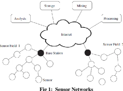
Sensor networks are dense wireless networks of small, low-cost sensors, which collect and disseminate environmental data. Wireless sensor networks facilitate monitoring and controlling of physical environments from remote locations with better accuracy. A node in Sensor Network is often not only responsible for data collection, but also for in-network analysis, correlation, and fusion of its own sensor data and data from other sensor nodes. When many sensors cooperatively monitor large physical environments, they form a wireless sensor network (WSN). Sensor nodes communicate not only with each other but also with a base station (BS) using their wireless radios, allowing them to disseminate their sensor data to remote processing, visualization, analysis, and storage systems[1]-[3].

Communication in wireless sensor network can achieved by makes use IEEE 802.11 family of standards which is the most common wireless networking technology for mobile systems. The different types of wireless sensor protocols uses different frequency for example, the 2.4-GHz band is used by IEEE 802.11b and IEEE 802.11g, while the IEEE 802.11a protocol uses the 5-GHz frequency band. IEEE 802.11 was frequently used in early wireless sensor networks and can still be found in current networks when bandwidth demands are high (e.g., for multimedia sensors). However, the high-energy overhead of IEEE 802.11-based networks makes this standard unsuitable for low-power sensor networks. The data rate requirements in sensor networks are comparable to the bandwidths provided by dial-up modems, therefore the data rates provided by IEEE 802.11 are typically much higher than needed. This has led to the development of a variety of protocols that better satisfy the networks’ need for low power consumption and low data rates. For example, the IEEE 802.15.4 protocol has been designed specifically for short range communications in low-power sensor networks and is supported by most academic and commercial sensor nodes[4]-[6].

redundant information or aggregation of data that may be smaller than the original data. Figure. 1 shows a representative Sensor Networks [3].

Fig 1: Sensor Networks

PSO is a metaheuristic as it makes few or no assumptions about the problem being optimized and can search very large spaces of candidate solutions. However, metaheuristics such as PSO do not guarantee an optimal solution is ever found. More specifically, PSO does not use the gradient of the problem being optimized, which means PSO does not require that the optimization problem be differentiable as is required by classic optimization methods such as gradient descent and quasi-Newton methods. PSO can therefore also be used on optimization problems that are partially irregular, noisy, change over time, etc. A basic variant of the PSO algorithm works by having a population (called a swarm) of candidate solutions (called particles). These particles are moved around in the search-space according to a few simple formulae. The movements of the particles are guided by their own best known position in the search-space as well as the entire swarm's best known position. When improved positions are being discovered these will then come to guide the movements of the swarm. The process is repeated and by doing so it is hoped, but not guaranteed, that a satisfactory solution will eventually be discovered.

2.BACKGROUND

STUDY

Particle swarm optimization (PSO) is a computational method that optimizes a problem by iteratively trying to improve a candidate solution with regard to a given measure of quality. PSO optimizes a problem by having a population of candidate solutions, here dubbed particles, and moving these particles around in the search-space according to simple mathematical formulae over the particle's position and velocity. Each particle's movement is influenced by its local best known position and is also guided toward the best known positions in the search-space, which are updated as better positions are found by other particles. This is expected to move the swarm toward the best solutions.

In 802.11b is probably the most popular wireless networking protocol in use today. Millions of devices supporting it have shipped since 1999. It uses a modulation called Direct Sequence Spread Spectrum (DSSS) in a portion of the ISM band from 2.400 to 2.495GHz. It has a maximum rate of 11 Mbps, with actual usable data speeds up to about 5 Mbps [7].

In 802.11g is a relative latecomer to the wireless market place. Despite the late start, 802.11g is now the de facto standard wireless networking protocol as it now ships as a standard feature on virtually all laptops and most handheld devices. 802.11g uses the same ISM range as 802.11b, but uses a modulation scheme called Orthogonal Frequency Division

Multiplexing (OFDM). It has a maximum data rate of 54 Mbps (with usable throughput of about 22Mbps), and can fall back to 11 Mbps DSSS or slower for backwards compatibility with the hugely popular 802.11b [8].

In 802.11a uses OFDM. It has a maximum data rate of 54Mbps, with actual throughput of up to 27 Mbps. 802.11a operates in the ISM band between 5.745 and 5.805 GHz, and in a portion of the UNII band between 5.150 and 5.320GHz. This makes it incompatible with 802.11b or 802.11g, and the higher frequency means shorter range compared to 802.11b/g at the same power. While this portion of the spectrum is relatively unused compared to 2.4GHz, it is unfortunately only legal for use in a few parts of the world. [9].

3.

CHALLENGES

AND

CONSTRAINTS

OF

WIRELESS

SENSOR

NETWORK

Sensor network are subjected to variety of unique challenges and constraints which helps to solve many problems by sharing many similarities with other distributed systems. The design of a wireless sensor network depends upon these constraints. The various design constraints of a wireless sensor network are Energy, Self Management, wireless Networking and decentralized Management [10].

Sensor network designs are based on the constraint that sensor nodes should operate with limited energy budgets. The sensor networks are powered through batteries, which must be either replaced or recharged (e.g., using solar power) when depleted. In sensor networks certain nodes are discarded once their energy source in the network is depleted. The energy consumption of sensor nodes affects when the battery can be recharged. A sensor node should be able to operate until either its mission time has passed or the battery can be replaced for non rechargeable batteries,. The length of the mission time depends on the type of application; It is possible for the wireless sensor network node to obtain energy sufficient for its operation directly from its environment. Such methods have been termed "energy scavenging" or "energy harvesting. Instead of using self contained energy nodes as battery powered nodes, Nowadays an Wireless Sensor Network node that employ energy scavenging to obtain sufficient energy. In a properly designed wireless sensor networks, the energy scavenging nodes are very small because they do not need to carry their energy with them. Energy available from the any environment may vary greatly, and may be interrupted during certain periods of time. Often, these interruptions are deterministic and predictable, such as shift change periods on a piece of vibrating equipment; in other cases, the interruptions are stochastic. A statistical approach is often used in stochastic interruption such that the probability of a power outage of a given length is modelled. This is due to that power from different environment is sufficient for operation cannot be guaranteed at all times, the designer must choose a level of reliability based on the model of the scavengeable source, and design the node to meet that requirement [11].

Sensor network must operate mostly in remote areas and harsh environments, without infrastructure support or the possibility for maintenance and repair. Due this the sensor nodes must be self-managing to, operate and collaborate with other nodes, and adapt to failures, changes in the environment, and changes in the environmental stimuli without human intervention by configure themselves in the network such a process is called as self management [12].

locations. Wireless telecommunications networks are generally implemented and administered using a transmission system called radio waves. This implementation takes place at the physical level (layer) of the network structure [13]-[14].

4.PROPOSED

METHODOLOGY

Regenerative techniques are used for localizing the node and calculate bit error rate (BER). A basic variant of the PSO algorithm works by having a population (called a swarm) of candidate solutions (called particles). These particles are moved around in the search-space according to a few simple formulae. The movements of the particles are guided by their own best known position in the search-space as well as the entire swarm's best known position. When improved positions are being discovered these will then come to guide the movements of the swarm. The process is repeated and by doing so it is hoped, but not guaranteed, that a satisfactory solution will eventually be discovered. Localizing and tracking is an essential object for a sensor network in many practical applications. Moreover, it is a familiar problem that can be used as a vehicle to study many information processing and organization problems for sensor networks. Tracking exposes the most important issues such as collaborative processing, information sharing, and group management including which nodes should sense, which have useful information and should communicate, which should receive the information and how often, and so on, which takes place in a dynamically evolving environment.

A sensor network in sensing and information processing can define as a tuple, G = {V, E, PV, PE}, V and E specify a network graph, with its nodes V, and link connectivity E α V × V. PV is a set of functions that characterizes the properties of each node in V, such as its location, computational capability, sensing modality, sensor output type, energy reserve, and so on. Possible sensing modalities include acoustic, seismic, magnetic, IR, temperature, or light. Possible types of sensor output include information about signal amplitude, source direction-of-arrival (DOA), target range, or target classification label. Similarly, PE specifies properties for each link, such as link capacity and quality.

We describe two common types of sensors for tracking: acoustic amplitude sensors and direction-of-arrival (DOA) sensors. An acoustic amplitude sensor node measures sound amplitude at the microphone and estimates the distance to the target based on the physics of sound attenuation. An acoustic DOA sensor is a small microphone array. Using beam-forming techniques, a DOA sensor can determine the direction from which the sound comes, that is, the bearing of the target. More generally, range sensors estimate distance based on received signal strength or time difference of arrival (TDOA), while DOA sensors estimate signal bearing based on TDOA. The nonparametric representation have poses few restrictions on the type of sensors to be used and allows the network to easily fuse data from multiple types of sensors. Relatively low-cost sensors such as microphones are attractive because of their affordability as well as simplicity in computation. However, there are no barriers to adding other sensor types, including imaging, motion, infrared (IR), or magnetic sensors. Low-cost, integrated imagers, or cameras, are attractive for target detection and identification because of the richness in the information an image can capture. Video cameras provide additional motion information that can be very useful in recognizing subtle behaviours of subjects. A sensor network can utilize a variety of sensing modalities to optimally sense phenomena of interest. For sensor network applications, a sensor may be characterized by properties such as cost, size, sensitivity, resolution, response time, energy usage, and ease of calibration and installation. One may have to carefully balance

the utility of a sensor with the cost of processing the data. A major consideration is whether the data processing involves only local data or requires data from a number of sensors. For example, to estimate the bearing of a target, one needs to combine measurements from several sensors through communication if the sensors are not on a single node. This adds to the cost of processing and places an additional requirement on time synchronization across nodes. To ground the discussions, we will study the acoustic amplitude and DOA sensors.

The concept behind the time of arrival (ToA) method (also called time of flight method) is that the distance between the sender and receiver of a signal can be determined using the measured signal propagation time and the known signal velocity. For example, sound waves travel 343 m/s (in 20 ◦C), that is, a sound signal takes approximately 30 ms to travel a distance of 10 m. In contrast, a radio signal travels at the speed of light (about 300 km/s), that is, the signal requires only about 30 ns to travel 10 m. The consequence is that radio based distance measurements require clocks with high resolution, adding to the cost and complexity of a sensor network. The one-way time of arrival method measures the one-way propagation time, that is, the difference between the sending time and the signal arrival time.

5.

EXPERIMENTS

AND

RESULTS

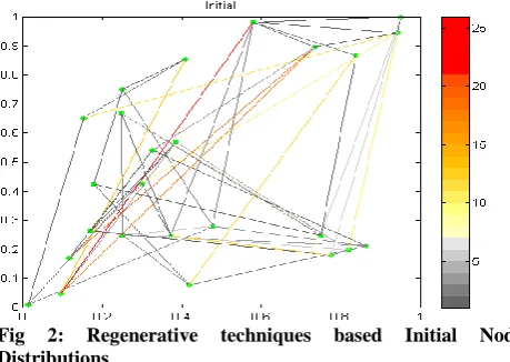
Figure. 2 shows Regenerative techniques based Initial Node Distributions.

Fig 2: Regenerative techniques based Initial Node Distributions

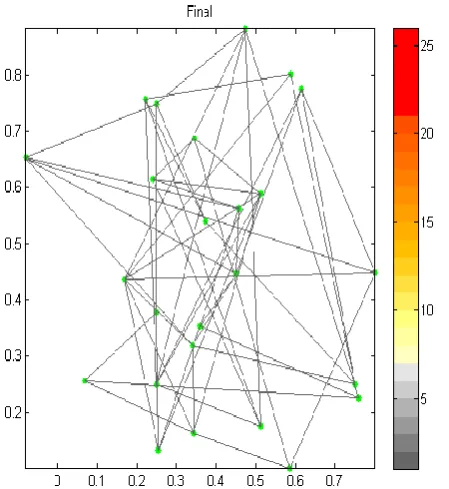
Fig 3: Regenerative techniques based Final Node Distributions

If we have a network topology we know the coordinates of each node in the topology and also the distance matrix between each node. However, as simulation input, we use only part of the distance matrix and choose three typical nodes as beacons. After that, we can evaluate the error distributions by comparing the estimated coordinates of each node and their original coordinates. Figure. 3 shows for Regenerative techniques based Final Node Distributions.

Fig 4: Iteration versus first order optimality

Fig 5: Regenerative Node Distribution function

By specifying the number of nodes, distance of grid unit and the random noise relative to the spacing of each grid, we can programmed to generate a random pattern of the network which means that we can get an array of nodes with the known co-ordinates and also we know the full distance matrix between any nodes. Figure. 4 show Regenerative Iteration versus first order optimality.

Fig 6: Iteration versus Preconditioned Conjugate Gradient (PCG) iterations per iteration

Fig 8: Regenerative Rounder filter versus original

We show that each distinct region formed in this manner can be uniquely identified by a location sequence that represents the distance ranks of reference nodes to that region. We present an algorithm to construct the location sequence table that maps all these feasible location sequences to the corresponding regions by using the locations of the reference nodes. This table is used to localize an unknown node (that is, the node whose location has to be determined) as follows. The unknown node first determines its own location sequence based on the measured strength of signals between itself and the reference nodes. It then searches through the location sequence table to determine the “nearest” feasible sequence to its own measured sequence. The centroid of the corresponding region is taken to be its location. Figure. 5 show Regenerative Node Distribution function.

Fig 9: Regenerative Iteration versus Curvature of current direction

We performed a variety of simulation experiments to cover a wide range of network (number of nodes), the radio range, and the distance measurement error and computation time. Figure. 6 show Iteration versus Preconditioned Conjugate Gradient (PCG) iterations per iteration.

The key metric for evaluating all the listed methods was the accuracy of the location estimates which versus the deployment, communication and computation cost. The table 1 shows the transmission ranges of different networks. Figure. 7 show Optimized filter versus original.

The localization error is denoted as LE. It is expressed as a percentage error. It is normalized with respect to the radio range to allow a comparison of results obtained for different size and range networks. Figure. 8 show Regenerative Rounder filter versus original.

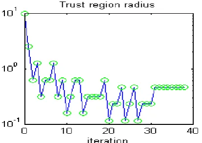
Fig 10: Regenerative Iteration versus trust region radius

Fig 11: Energy per bit to noise power spectral density ratio ( Eb/No) versus BER

The value of the transmission range r determines the number of neighbours of each node in the network. The radio range considered from the interval [0.21 – 0.02]. Figure. 9 show Iteration versus Curvature of current direction.

Table 1. Localization Error versus Computational Time

Number of

Nodes

Localization error LE

Computational Time [s]

150 0.113 0.856

250 0.124 0.978

550 0.135 1.623

1500 0.146 2.857

1800 0.157 3.969

Received signal strength (RSS) measurements estimate the distances between neighbouring sensors from the received signal strength measurements between the two sensors. Received signal strength indicator (RSSI) has become a standard feature in most wireless devices. The RSS based localization techniques eliminate the need for additional hardware, and exhibit favourable properties with respect to power consumption, size and cost. As such, the research community has considered the use of RSS extensively. In general, the RSS based localization techniques can be divided into two categories: the distance estimation based and the RSS profiling based techniques. Received signal strength indicator (RSSI), is a commonly found feature in wireless devices which can be used to measure the amplitude of the incoming radio signal. Figure. 11 shows Transmit versus receive diversity.

Fig 12: Transmit versus receive diversity

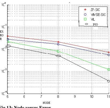
The primary technology used for building low-cost wireless networks is currently the 802.11 family of protocols, also known in many circles as Wi-Fi. The 802.11 family of radio protocols (802.11a, 802.11b, and 802.11g) have enjoyed an incredible popularity in the United States and Europe. By implementing a common set of protocols, manufacturers worldwide have built highly interoperable equipment. This decision has proven to be a significant boon to the industry and the consumer. Consumers are able to use equipment that implements 802.11 without fear of “vendor lock-in”. As a result, consumers are able to purchase low-cost equipment at a volume which has benefitted manufacturers. If manufacturers had chosen to implement their own proprietary protocols, it is unlikely that wireless networking would be as inexpensive and ubiquitous in today scenario. While new protocols such as 802.16 (also known as WiMax) will likely solve some difficult problems currently observed with 802.11, they have a long way to go to match the popularity and price point of 802.11 equipment. As equipment that supports WiMax is just becoming available at the time of this writing, we will focus primarily on the 802.11 family. There are many protocols in the 802.11 family, and not all are directly related to the radio protocol itself. Fig.12 shown Node versus Error.

Fig 13: Node versus Error

As the node listens to its neighbours, a node present on the side of the grid will have fewer neighbours to listen to, and thus will have a poor accuracy. Increasing the global density will increase the number of nodes close to the edges, but will also increase the presence of beacons. This results on more beacons available for the edge nodes, and then in a better accuracy.

CONCLUSION

REFERENCES

[1] Chan. K. W. and H. C. So, 2009 “Accurate distributed range-based positioning algorithm for wireless sensor networks,” IEEE Transactions on Signal Processing, vol. 57, no. 10, pp. 4100–4105.

[2] Cheung. W, H. C. So, W. K. Ma, and Y. T. Chan, 2006 “A constrained least squares approach to mobile positioning: algorithms and optimality,” EURASIP Journal on Applied Signal Processing, vol. 2, Article ID 20858, pp.23.

[3] Costa. A, N. Patwari, and A. O. Hero III, 2006 “Distributed weighted-multidimensional scaling for node localization in sensor networks,” ACM Transactions on Sensor Networks, vol. 2, no. 1, pp. 39– 64.

[4] Drineas. P., A. Javed, M. Magdon-Ismail, G. Pandurangan, R. Virrankoski, and A. Savvides, 2006 “Distance matrix reconstruction from incomplete distance information for sensor network localization,” in Proceedings of the 3rd Annual IEEE Communications Society on Sensor and Ad Hoc Communications and Networks (Secon '06), vol. 2, pp. 536–544.

[5] Khan. A, S. Kar, and J. M. F. Moura, 2009 “Distributed sensor localization in random environments using minimal number of anchor nodes,” IEEE Transactions on Signal Processing, vol. 57, no. 5, pp. 2000–2016.

[6] Lui. K. W. K., F. K. W. Chan, and H. C. So, 2009 “Semidefinite programming approach for range-difference based source localization,” IEEE Transactions on Signal Processing, vol. 57, no. 4, pp. 1630–1633.

[7] Lui. K. W. K., W.-K. Ma, H. C. So, and F. K. W. Chan, 2009 “Semi-definite programming algorithms for sensor network node localization with uncertainties in anchor positions and/or propagation speed,” IEEE Transactions on Signal Processing, vol. 57, no. 2, pp. 752–763.

[8] Sun. M. and K. C. Ho, 2009 “Successive and asymptotically efficient localization of sensor nodes in closed-form,” IEEE Transactions on Signal Processing, vol. 57, no. 11, pp. 4522–4537.

[9] Tseng. P, 2007 “Second-order cone programming relaxation of sensor network localization,” SIAM Journal on Optimization, vol. 18, no. 1, pp. 156–185.

[10]Wang T, G. Leus, and L. Huang, 2009 “Ranging energy optimization for robust sensor positioning based

on semi definite programming,” IEEE Transactions on Signal Processing, vol. 57, no. 12, pp. 4777–4787.

[11]Wang T, G. Leus, D. Neirynck, F. Shu, and L. Huang, “Ranging energy optimization for robust sensor positioning, 2009 ” in Proceedings of IEEE International Conference on Acoustics, Speech, and Signal Processing (ICASSP '09), pp. 2237–2240.

[12]Whitehouse. K., C. Karlof, and D. Culler, 2007 “A practical evaluation of radio signal strength for ranging-based localization,” ACM SIGMOBILE Mobile Computing and Communications Review, , vol. 11, no. 1, pp. 41–52.

[13]Yang. K., G. Wang, and Z. Q. Luo, 2009 “Efficient convex relaxation methods for robust target localization by a sensor network using time differences of arrivals,” IEEE Transactions on Signal Processing, vol. 57, no. 7, pp. 2775–2784.

[14]Zein-Sabatto. Z, V. Elangovan, W. Chen, and R. Mgaya, 2009 “Localization strategies for large-scale airborne deployed wireless sensors,” in Proceedings of IEEE Symposium on Computational Intelligence in Multi-Criteria Decision-Making (MCDM '09), pp. 9– 16.

AUTHORS PROFILE

Mr. J.Jasper Gnana Chandran received his B.E from M.S University, M.E from Anna University Chennai, Tamilnadu, India. Currently he is working as Professor & Head in EEE dept in Francis Xavier Engineering College, Tirunelveli, Tamilnadu. He is pursuing his Ph.D degree in Bharathiyar University, Tamilnadu, South India in the area of Sensor Networking. He has published several papers in national conferences, international journals and also he has written a book in Electrical Engineering. His area of interest includes Control System, Sensor network and Wireless Networking.He is a member in ISTE. He has organized Several Conferences and Seminars at national and state level.