International Parities and Exchange Rate Determination

(1)

Munich Personal RePEc Archive

International Parities and Exchange Rate

Determination

Zhao, Yan

31 March 2005

(2)

International Parities

and

Exchange Rate Determination

Yan Zhao

*

Abstract

The model of equilibrium exchange rate combining purchasing power parity (PPP)

and uncovered interest parity (UIP) is widely tested using the cointegration approach.

Most of the recent studies, however, are deficient in the treatment of expectations and

the power of tests.

This paper aims at resolving the two deficiencies by deriving and testing the

yen/dollar exchange rate model. Perfect foresight is assumed to circumvent the

expectation problem and a modification of cointegration variables is introduced to

improve the power of tests.

With this new methodology, supportive evidence for the hypothesis of combining

PPP and UIP is found in the short run: cointegration between the future exchange rate,

price and interest rate differentials exists; the error correction model (ECM) is

significant. The paper also suggests that it is the interest rate differential, rather

than the price differential, that explains more of the movement of the nominal

exchange rate in the short run. In the long run, however, the cointegration does not

exist because the interest rate differential becomes exogenous.

*

(3)

Acknowledgements

This paper is written under the supervision of Professor Hiroshi Shibuya at the Otaru University of Commerce. I still remember the days when he held two seminars per week for me last year: International Finance and Time-Series Econometrics, without which I could not have begun this research. I think he is a great instructor in keeping the balance between intriguing the student’s interest and teaching hard materials. His instruction is highly appreciated.

Moreover, Professor Shibuya made many important suggestions and remarks on this paper. It was my first time to write a research paper and during the writing process, what he gave me was hints rather than instructions. He never told me what I should do or should not do. Instead, he gave me full latitude to try my own idea. I realize now that working out one’s own idea is really important to do research. It is the combination of his supervision and my own work that produced this paper.

(4)

1. Introduction

Recently the question of exchange rate determination has been extensively researched. Knowing the level of equilibrium exchange rate is becoming an important issue in the field of international finance and macroeconomics, especially with the more integrated world economy. It is of vital importance not only for individuals and firms engaging in international trade and finance, but also for the monetary authorities conducting monetary policy. Moreover, the equilibrium exchange rate is an important macroeconomic policy variable for both developing and developed countries. As a result, almost all open macroeconomic theories involve the measurement of equilibrium exchange rate.

1.1. PPP as the First Exchange Rate Model

In the economic literature, purchasing power parity (PPP), which was put forth by Cassel (1921)1_{, is the first theory to measure the equilibrium exchange}

rate level. Based on the law of one price (LOP), purchasing power parity states that the relative price determines the exchange rate movement.

According to the PPP hypothesis, the relative price is the main determinant of the exchange rate and if written in log forms, the exchange rate should be equal to the price differential. The common deviation of the exchange rate from the relative price and the more volatile exchange rate fluctuation in the post-floating period, however, prompted many economists to test the validity of purchasing

1_{Gustav Cassel 1921.}

The World’s Monetary Problems. London: Constable.

(7)

power parity2_{. Recent tests of PPP have been typically based on the}

investigation of the time series property of the real exchange rate, which can be seen as the residuals from PPP. These test results3_{indicate that PPP may not}

hold: the real exchange rates are not always stationary. The failure of PPP in the short run is common. Even in the long run, the validity of PPP is mixed.

1.2. Combining PPP with UIP (CHEER)

The failure of PPP caused many people to raise doubt on the PPP as the model of equilibrium exchange rate. With the great expansion of world financial markets in the past twenty years, some economists put forward a model of equilibrium exchange rate that combines the purchasing power parity and uncovered interest parity (UIP). UIP is derived on the assumption of foreign exchange market efficiency, i.e., there is no “excessive arbitrage opportunity”. UIP states the relationship between the exchange rate and the interest rate differential, indicating that an increasing domestic to foreign interest rate differential will generate expected depreciation of the exchange rate.

The proponents of the model that combines PPP and UIP argue that PPP represents the equilibrium of goods market only. They suggest that the price levels are not sufficient to capture all the factors causing fluctuations of the exchange rate without taking the world financial markets into account. According to their arguments, the exchange rate deviation from PPP is not

2

Engel and Morley (2001) proposed a different view and they developed a model to show that the nominal exchange rate converges much more slowly than the prices.

3_{See Chapter 2 of this paper for more details of the literature survey of PPP.}

(8)

surprising because of the existence of non-zero interest rate differentials.

The model that combines PPP and UIP reflects the idea that although PPP serves as an important measurement of the exchange rate movements, its predictive power can be enhanced by allowing for the effects of financial markets when calculating the equilibrium exchange rate level. This methodology, therefore, is called as the capital enhanced equilibrium exchange rate (CHEER)

approach by MacDonald (2000). We adopt this terminology hereto in this paper. The CHEER approach was first proposed by Juselius (1991) and then developed by Johansen and Juselius (1992). Since then, the CHEER approach has become popular among economists in the field of exchange rate determination (See Chapter 2 for literature survey).

1.3. Two Problems of the CHEER Approach

Almost all papers on the CHEER approach try to find supporting evidence by searching for cointegration relationship among exchange rate, price and interest rate differentials. Those papers, however, have two major problems.

The first problem is an inappropriate treatment of expectation in the cointegration model. The cointegration relationship is often investigated between prices, interest rates and the contemporaneous, not the expected future exchange rate. Since UIP states the relationship between interest rates and

expected future exchange rate, their cointegration models are not consistent with the UIP hypothesis. Therefore, their models do not combine PPP and UIP theories correctly.

(9)

The second problem is that their studies lack the power of rejecting the null hypothesis of no cointegration, casting doubt on the validity of CHEER hypothesis. Careful reading of those papers4_{reveals that the failure of}

cointegration often occurs in short data span while cointegration often becomes apparent in the longer data span. The contingent property on data span has the same similarity as PPP and UIP, which are also believed to be long-run phenomenon5_{. Is it possible that the failure of PPP or UIP causes the}

non-rejection of no cointegration6_?

This paper shows that either a failure of PPP or UIP does result in non-rejection of no-cointegration. The reason is that the linear sum of error terms in PPP and UIP will not be stationary if exactly one of them fails to hold7_.

In this case, it is impossible to find evidence supporting the CHEER approach since the null of no cointegration cannot be rejected. If either PPP or UIP fails to hold, the variables in the cointegration analysis need to be modified to increase the possibility of finding cointegration. Thus, an appropriate step in the investigation of whether PPP and UIP hold is essential to improve the power of cointegration analysis. Since PPP and UIP are rather long-run than short-run phenomenon, we expect that it is necessary to distinguish the CHEER models according to the data span.

4

See Section 2.3 of this paper.

5

Most people believe PPP is a long-run phenomenon because price adjustment takes time. The conclusion about whether UIP is also a long-run phenomenon is not necessarily widely accepted, although some people find that UIP tends to hold better with longer data span.

6

This sentence contains two “no” and looks awkward. It is technically accurate, however, since the null hypothesis of no cointegration is always tested in the CHEER approach. If the null hypothesis is rejected, we find supporting evidence of CHEER approach and vice versa.

7

Either PPP or UIP fails, not both of them. The linear combination of the PPP and UIP errors can be cointegrated if both of them are nonstationary.

(10)

1.4. Solution of the Two Problems

This paper aims at solving the above two problems in the CHEER approach. The first problem of expectation is circumvented in a straightforward way by introducing expectation in terms of perfect insight. The future nominal exchange rate is thus taken as the substitute for the expected future exchange rate. Expectation is necessary to represent UIP correctly and in some CHEER paper, an expectation is formed on the price differentials (See Stephens, 2004, for example.). In reality, however, people do not always focus on goods markets because price level changes in all items are not easy to observe. It is quite possible for them to expect future exchange rate changes from financial markets8_.

Moreover, the price level based expectation is prone to cause systematically expectation errors in the presence of “sticky domestic price” (Obstfeld and Rogoff, 1996).

The second problem of the lack of power in tests is solved by distinguishing the short-run (post-floating period since 1973) model from that of long-run (past 130 years) model because PPP is tested to hold only in the latter. PPP’s failure in the short run prompts us to modify the CHEER model. The modified short-run model is new in that it is a differenced model of that of the long run. The effect of the modification becomes apparent: we could not have rejected the null hypothesis of no cointegration if using the same model as the long run. Moreover, the coefficients of the error correction model (ECM) in the short run are

5 8_{The idea that people foresee future exchange rate from financial markets comes from the}

(11)

significant, strongly supporting the validity of the CHEER approach.

The conclusion of the long-run analysis is a surprise: we can not reject the null of no cointegration although both PPP and UIP hold. Therefore, the CHEER approach fails. The econometric analysis reveals that this is because the relative interest becomes exogenous in the long run and it does not belong to the exchange rate determination system. The failure of the CHEER approach in the long run suggests that we should be careful about combining PPP and UIP when analyzing the historical data, in which the world financial markets are under-developed.

The remainder of this paper is structured as follows. Chapter 2 gives the literature survey of the PPP, UIP and CHEER approaches. Chapter 3 analyzes the short-run model. Chapter 4 analyzes the long-run model. Chapter 5 summarizes this paper.

(12)

2. Literature Survey

2.1 Review of PPP

2.1.1. What’s PPP?

Purchasing Power Parity (PPP), which addresses the relationship between nominal exchange rate and prices, is one of the most important theoretical building blocks in international finance. The basic idea of PPP can be traced back as far as the writing of “Wealth of Nations” by Ricardo in the 19th_century

(Mark, 2001). The term PPP, however, was first introduced by Cassel (1921). Based on the hypothesis of law of one price (LOP), PPP states that one good should be sold at the same price in domestic and foreign markets if denominated by the same currency. If we denote the domestic and foreign price levels by and , respectively. And if represents the nominal exchange rate (foreign price of domestic currency), then PPP implies:

t

P

*

t

P St

*

t t

P =S P_t

t

(1) More frequently, PPP is expressed in the logarithm forms. By changing to lower-case letters to denote the natural logs and isolating the exchange rate as the left-hand variable, we obtain:

s_t = p_t− p* (2) Traditionally, equation (1) and (2) are referred as the absolute PPP and by taking first differences of (2), we get the relative PPP:

*

t t

s p p_t

∆ = ∆ − ∆ (3) Equation (2) and (3) are simple in that only two variables, the nominal exchange rate and price levels, are involved. The nominal exchange rate is

(13)

definite. The price levels, however, vary in a large degree and the selection of the price index is not unanimous. Cassel9_{suggested the general price level,}

whether or not it contains prices of non-tradable goods. Many people use the consumer price index (CPI) in empirical studies. However, some people argue that the price index of tradable goods is more appropriate because of the Balasa-Samuelson Effect (1964). For example, Hau (2000) pointed that the large exchange rate fluctuation can be attributed to the existence of non-tradable goods. Kim and Ogaki (2004) showed that the half-lives for the real exchange rate based on producer price index are shorter than that based on CPI, the former of which is believed to contain more tradable goods.

The CPI is the only price level available for the data spanning over one century. And this is a practical reason for researchers to choose CPI when investigating long-run PPP hypothesis in addition to Cassel’s original argument. This paper also selects CPI to make the long-run (from 1870) analysis consistent with the short-run analysis.

2.1.2. Empirical tests of PPP

With the development of time-series econometrics, recent tests for PPP have often been conducted by investigating whether it is possible to reject the null hypothesis of unit root in the real exchange rate. The logarithm of real exchange rate,q_t, can be defined as:

8 9

The following Cassel’s saying is excerpted from Frenkel’s paper (1978):“Some people believe that Purchasing Power Parities should be calculated exclusively on price indices for such commodities as for the subject of trade between the two countries. This is a

(14)

*

t t t

q = −s p + p_t (4) Comparing equation (2) and (4) reveals that the real exchange rate q is equivalent to the deviation of PPP. Therefore, testing for PPP becomes the investigation of time series property of the real exchange rate: If the real exchange rate is tested to be stationary, we find evidence supporting PPP. Unit root test was first introduced into the test of PPP by Roll (1979) and later by Adler and Lehmann (1983). The unit root test approach has been popular in the past two decades.

t

Unit root tests on the real exchange rate do not seem to be in favor of PPP: almost all of the short-run tests are unable to reject the null hypothesis of unit root, especially since the post-floating period exhibits large and persistent departure. Even in the long run, the evidence supporting PPP is mixed. These results led many economists to seek explanations for the failure of PPP.

t

q

In general, the failure of PPP is ascribed to the transportation costs, the existence of trade barriers and fixed exchange rates, and so on. Vast literature have been written on the “law of one price”, which is the basic assumption of PPP10_{. For example, Isard (1977) provided striking evidence of the violation of}

“law of one price” from the U.S., Germany, Japan and Canada data. Engel and Rogers (1996) studied the U.S. and Canadian consumer price data and found that the law of one price generally failed11_{. Another explanation originates from}

Dornbush’s influential “overshooting” model (1976)12_{, which states that the}

monetary policy can enlarge the real exchange fluctuation.

10

See Froot, Kim and Rogoff (1995) and Rogoff (1996) for survey of deviation from law of one price or “border effect”.

11

Engel showed that the prices of similar goods in two countries are more volatile than that of dissimilar goods within the same country.

12_{The overshooting model is later extended by Obstfeld and Rogoff (1995).}

(15)

Some economists, however, began to take doubt on the unit root tests because the failure of PPP is still common. Frankel (1986) put forward a serious question about the unit root test, i.e., the lack of power problem. He pointed out that short data span used to examine the real exchange rate may not be long enough to reject the null hypothesis of unit root, even it is truly stationary.

Frankel’s idea is later developed by some other economists. According to their argument, many economists have attempted to solve the data span problem13_{. Two ways have been widely used to circumvent this problem. One}

way is to use data of a longer span14_{. Frankel (1996), Edison (1987) and Lothian}

and Taylor (1996) have successfully rejected the null of random walk of the real exchange rate by using data longer than one century. The technique of increasing the data span, however, has been criticized because of the existence of various exchange regimes and structural breaks due to real shocks on so long a data span. For example, Papell and Prodan (2004) find that evidence of PPP can be increased from 9 to 14 out of 16 countries when allowing for structural breaks.

The other method of circumventing the data span problem is to use panel data, i.e., to increase the number of real exchange rates under the unit root test. The panel data technique was first proposed by Abuaf and Jorion (1990) and later developed by Levin and Lin (1993), Im, Pesaran and Shin (1997), and Maddala and Wu (1999). Some of these studies provided evidence supporting PPP. Panel data method need to be applied with some reserve, however, as this technique has two pitfalls. One is that the rejection of the null hypothesis of

13

For example, see Lothian (1986), Froot and Rogoff (1995), Lothian and Taylor (1997).

14

Only increasing the observation frequency without extending the data span can not

improve the test power.

(16)

unit root cannot be logically interpreted that all of the real exchange rates under consideration are stationary. It only implies that at least one series of the real exchange rate is stationary. The other pitfall of the panel data test is that the small sample size distortion15_{problem will aggravate when more than one series}

of real exchange rates are examined.

Some people tested relative PPP in the belief that the trend in the real exchange can be removed by differencing. For example, Coakley et al. (2003) argues that the inflation differential will cause the nominal exchange rate to move proportionally even if important real shocks existed. This paper also tested relative PPP in the short run when strict PPP is tested to fail.

In recent years, there is a trend that some economists tried to test PPP in two new ways: non-linear method16_{and laboratory test (Fisher, 2001). Non-linear}

proponents argue that there are probably potential sources of nonlinearity in real exchange rates. For example, the imperfect mobility of international trade and the heterogeneous behavior in the foreign exchange market both create a band within which the exchange rate becomes extremely capricious. Fisher, one of the laboratory test pioneers, finds that both strict PPP and relative PPP holds well with the experimental data. He points that it is because the data in the laboratory is more “unambiguously accurate” and the environment is more “static” compared with the true data17_{. The non-linear adjustment method and}

laboratory test certainly leave room for further research.

15

Schwert (1989) proposed the small size distortion problem in unit-root tests.

16

See Michael et al. (1997), Sarantis (1999), Baum et al (2001), Taylor et al. (2001) and Bec et al. (2004).

11 17

(17)

2.2 Review of UIP

2.2.1. What’s UIP?

Uncovered Interest Parity (UIP) is derived from an equilibrium condition in international financial markets. Let It and

*

t

I denote the domestic and foreign interest rates, respectively, and represents the expectation of nominal exchange rate at period (t+1), then UIP states:

1 (

t t

E s₊ )

* ( 1

1 (1 ) t t

t t

t

E S I I

S

+

+ = + ) (5)

Equation (5) can be interpreted as that one unit of currency should have the same return whether invested in the domestic or the foreign markets at equilibrium. UIP equation is more often written in its log forms:

* 1

( )

t t t t t

E s₊ − = −s i i (6) wherelogE St( t+₁)=E st( t+₁), logSt =st, log(1+It)=it and

* * log(1+It)=it .

Equation (6) gives the more apparent interpretation of UIP, i.e., the domestic and interest rate must be higher (lower) than the foreign interest rate by an amount equal to the expected depreciation (appreciation) of the domestic currency. If we use the forward exchange rate instead of the expected future rate, we get Covered Interest Parity (CIP):

t

F

*

t t t t

f − = −s i i (7) where ft =log( )Ft . The comparison of equation (6) and (7) suggests that test of

UIP is equivalent to test whether ft =E st( t+₁).18

12 18

(18)

2.2.2. Empirical test of UIP

Although UIP implies the foreign exchange market efficiency, what Mark (2001) defines “there are no unexploited excess profit opportunities”, empirical analysis reveals that violations of UIP are common and they present an important empirical puzzle in international finance.

Economists have presented various explanations for these apparent failures. Mark (2001) classified them into three reasons. The first is that the forward foreign exchange rate contains a risk premium. This argument says that UIP is derived under the hypothesis of risk neutral agents; in real foreign exchange markets, however, risk averters are more common. Risk averters demand a risk premium for the bearing of risky currencies. Engle Robert F. et al (1987) argues that the risk premium is time variant using ARCH-M model. Ogaki (1999) shows that the substitution between domestic and foreign bonds can be strong because of the potential risk. The literature on risk premium is vast (See the survey paper of Engel, 1996).

The second reason is the violation of the perfect information assumption. The real economy environment always changes but people will need time to know these changes and to adjust their behavior. During the learning and adjustment period, it is not a surprise that individuals make systematic prediction errors even though “they behave rationally”. Ascribing the failure of UIP to the individual’s incomplete understanding of the economy due to imperfect information is called the “peso-problem” approach, which was originally studied by Krasker (1980) and later developed by Lewis (1989). Krasker observed the interest rate differential between the Mexican peso and the U.S dollar and

(19)

showed that if the monetary authority would abandon the pegged exchange rate system, we could see the sequence of “systematic, serially correlated but rational forecast errors”. Lewis proposes that the individuals may be unaware of the shift in economic fundamentals in the beginning, which can be associated with the economic or political environment. Individuals need time to learn this shift and during the adjustment period, rational forecast errors tend to be serially correlated and systematic.

The third explanation is that some market participants are actually “irrational” for the reason that they rely on the extraneous information (for example, rumor), not economic fundamentals, to predict the asset value. The individuals who do not behave irrationally are called “noise’’ traders, a name originally used by Black (1986). Black argued that the real world is too complicated for some (noise) traders to distinguish between the“pseudo and true” signals. Black suggested further that “noise” trader would generate excessive pseudo-signals, causing overdue optimism and pessimism. Therefore, the financial markets will be distorted by these “noise” traders and the exchange rate will deviate more from the valued based on the economic fundamentals. De Long et al. (1990) devised an overlapping generation model to study the pricing of foreign exchanges when “noise” traders generate excess trading volume and currency returns. Mark and Wu (1998) developed their model and used survey data to confirm that the “noise” traders caused spot and forward exchange dynamics.

In addition to the reasons aforementioned, some other economists argue that the failure of UIP lies in the data span. UIP is a long-run rather than a short-run phenomenon; therefore short span data is not appropriate. For

(20)

example, Alexius (2001) found supporting evidence for UIP using long-term government bond yields of 13 industrialized countries19_{. Meredith and Chinn}

(1998) researched on long-maturity bonds for G-7 countries and all the coefficients on interest differentials are of correct sign.

2.3 Cointegration Analysis of PPP and UIP

As stated beforehand, PPP concentrates on the goods market, while UIP emphasizes the financial markets. Some economists have tried to link them in a multivariate framework involving cointegration20_{and this approach is referred}

as a capital enhanced equilibrium exchange rate (CHEER). The approach captures the basic Casselian view of PPP that an exchange rate may be away from its PPP determined rate because of non-zero interest rate differentials21_.

In terms of balance of payments, the combination of PPP and UIP represents the interaction between current and capital account, respectively.

Johansen and Juselius (1992) are pioneers to combine PPP with UIP. They analyzed the long-run foreign transmission effects between the United Kingdom and the rest of the world and Juselius (1991) considered similar issues for Denmark and Germany; both focused on the long-run relations of PPP and UIP. Johansen and Juselius show that if PPP and UIP holds, then there will be two cointegration relationships among the following five variables:p_t, *

t

p , , and . The two cointegration vectors are: (1,-1,-1,0,0) and (0,0,0,1,-1) to represent

t

s i_t

*

t

i

19

Alexius’s paper deals with coupon payments in the long-term government bonds.

Allowing coupon payments to affect the length of the investment period rather than the bond price, UIP holds better.

20

We call two series cointegrated if they are integrated of the same order and the residual from their long-run relationship is stationary.

21_{See Officer (1976) for a detailed discussion of the Casselian view of PPP.}

(21)

PPP and UIP hypothesis, respectively.

The cointegration approach has been conducted by some other economists later, most of which did not prove well. Messe and Rogoff (1988) could not find cointegration between the real exchange rate and real interest rate differential among the dollar, yen, and Deutsche mark. Campbell and Clarida (1987) find that the interest differential is not sufficient to explain the volatility of dollar exchange rate. Edison and Pauls (1993) allowed for current accounts in the cointegration approach to obtain negative results. Ledesma et al (1998) studied the Spanish case but found no cointegration among the exchange rate, price and interest differentials.

Some more recent studies yield promising results using CHEER approach. Cheng (1999) researched on yen/dollar case and found no causality between prices and exchange rates in the short run. However, causality is found running from relative prices to exchange rates along with interest rates in the long run. Juselius and MacDonald (2000) investigated dollar-mark relationship and found that a significant price adjustment towards equilibrium exchange rate level is compensated by long-term bond rates. Caporale et al (2001) investigated the German mark and Japanese yen to find evidence favorable to PPP and UIP with the aid of cointegration approach. Aysun and Ozmen (2002) studied the Turkish case and they found cointegration relationship among prices, interest rates and exchange rate with dollar. Their finding also suggests that PPP and UIP do not hold if tested separately.

In most of these papers, cointegration is searched between the

contemporaneous exchange rate, price and interest rate differentials. Since UIP states the expected future rate, this cointegration does not represent PPP and

(22)

UIP hypothesis well. Taking aside this inappropriate treatment of expectation, conclusion about whether the cointegration relationship exists is mixed, causing some people to doubt the validity of the CHEER hypothesis. Is CHEER hypothesis misleading or the cointegration method lacks test power?

Careful review of these papers will suggest that all the papers succeeding in finding cointegration investigate the long-run phenomenon. Since PPP and UIP are believed to hold well in the long data span, we can expect that both of them hold in these papers, although they are not always explicitly tested. If both PPP and UIP do hold, there is no test power problem and cointegration relationship is easy to be detected, if there is any22_{. In the short data span, however,}

straightforward search of cointegration between exchange rate, price and interest rate differentials may fail due to the failure in either PPP or UIP. Cheng’s paper (1999), for example, is unable to find cointegration in the short run but finds cointegration in the long run. Here it is important to note that when both PPP and UIP fail, it becomes possible to find evidence of supporting CHEER (Aysun and Ozmen, 2002, for example). The reason is that the sum of the two nonstationary residuals in PPP and UIP may be stationary because of the interaction of goods market and financial market.

Thus, we should modify CHEER approach to solve the lack of power in tests before concluding that the CHEER hypothesis is inappropriate. It is quite possible that the inappropriate treatment of expectation and the lack of test power explain the unsatisfactory results of the recent papers. This paper attempts to test this new hypothesis by solving the two deficiencies.

22

It is also worth pointing out that cointegration may not necessarily exist when both PPP and UIP holds. See Chapter 4 for this paper.

(23)

3. Short-Run Analysis (Jan. 1973~Jun. 2004)

This section analyzes the floating period from January 1973 to June 2004. The data set contains the monthly nominal exchange rate, U.S and Japan’s consumer price index and nominal interest rate23_{. In this paper, Japan is taken}

as the domestic country.

3.1. Pretests of PPP and UIP

3.1.1.

t

Unit root process and Dickey-Fuller test

If PPP holds between U.S. and Japan, the shocks to yen’s real exchange rate,q , should be temporary in that will be mean-reversion. Specifically is called stationary if it exhibits mean reversion and has a finite variance. A unit root process is not stationary. Consider the simple AR (1) process:

t qt qt

1

t t

q =ρq₋ +ε (8) where we assume that − ≤ ≤1 ρ 1 and ε_t is white-noise with the variance of

σ . By introducing the lag operator, L24_{, we rewrite the above equation as:} (1−ρL q) t =εt

When q_t is stationary, the autoregressive polynomial (1−ρL) should be invertible, which requires thatρ<1. Then it is equivalent to say that the root L

in the autoregressive polynomial (1−ρL) lies outside the unit circle. Ifρ =1, then q_t becomes a random walk process,∆ =q_t ε_t, and

1

t

t i

q ε_t

=

∑

if we

k

23_{Considering a growing importance of international financial markets, I use the euro rates}

in this section.

24

For any variable ,qt .

k t t

L q =q₋

(24)

assume q₁ =0. Thus,

γ =

2

1 1

( )t var( t t ... )

Var q = ε ε+ ₋ + +ε =tσ

Therefore, is no longer stationary because the variance depends on t. We should be careful about the nonstationary variables because there might be what Granger and Newbold (1974) called a spurious regression. A spurious regression has significant t-statistics and a high

t

q

2

R , but the process is without any economic meaning. Therefore pretesting for nonstationarity the variables in a regression equation is of extremely importance. There are many kinds of unit-root tests and we first introduce the Dicker-Fuller (DF) test since it is the most straightforward and it is also the foundation of many other more complicated tests.

DF test begins by subtracting q_t₋₁ from each side of equation (8) and then consider:

1

t t

q γq₋ ε_t

∆ = + (9) where ρ−1. The parameter γ is of interest; if γ =0, the q sequence

contains a unit root. The test involves estimating equation (9) using OLS in order to obtain the estimated value of

t

γ and the associated standard error. By comparing the resulting t-statistic with the appropriate value reported in the DF tables25_{, we can determine whether to accept or reject the null hypothesis} γ _=0.

3.1.2. Nonstationary process and PPP test

After introducing the basic property of unit root and its test method, we proceed to conduct some unit root tests on the yen/dollar real exchange rate.

t

19 25_{DF table contains three sub-tables for three different regression equations, respectively.}

(25)

Some tests used in the following sections will be more complicated and powerful than the DF test.

3.1.2-1

The DF test

We add a constant to the right side of equation (2) and regress the nominal exchange rate s_t on a constant and the price differential(pt−p*t),

*

( )

t t t

s = +α β p − p +ε_t (10) to obtain: α =5.5767(348.3208) and β =1.6144(36.0596) with in the parenthesis. PPP requires that:

t−value

1

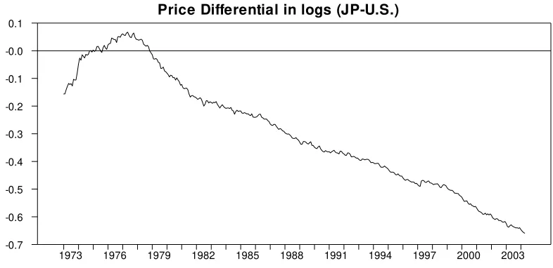
β = (11) The restriction is binding; however, the F-statistics value 188.3298 of equation (11) exceeds the 5 percent critical value of the 3.84 in the statistical table. Let denotes the real exchange rate and we depict the graph of the nominal and real exchange rates and price differential as Figure 1.

*

t t t

t s p p

[image:25.595.98.490.552.749.2]

q = − +

Figure 1-A

Nominal and Real Exchange Rate in logs (Yen/Dollar)

1973 1975 1977 1979 1981 1983 1985 1987 1989 1991 1993 1995 1997 1999 2001 2003 4.4

4.6 4.8 5.0 5.2 5.4 5.6 5.8 6.0

nominal real

(26)

[image:26.595.96.489.114.305.2]

Figure 1-B

Price Differential in logs (JP-U.S.)

1973 1976 1979 1982 1985 1988 1991 1994 1997 2000 2003 -0.7

-0.6 -0.5 -0.4 -0.3 -0.2 -0.1 -0.0 0.1

Source: DataStream and the author’s calculation

We test for the unit root according to equation (9) ∆ =q_t γq_t₋₁+ε to obtain:γ =-2.19143. Comparing the value of γ with the DF table implies that we can not reject the null of unit root process inq_t, because the absolute value of

γ is smaller than that of the 10 percent critical value , not to mention the 5 and 1 percent critical values .

(-2.571)

(-2.87 and -3.44)

3.1.2-2 The Augmented DF test

Not all time-series processes can be well represented by the first-order autoregressive process∆ =q_t α γ₀+ q_t₋₁+α₁t+ε_t. When we test unit roots in higher order equations such as the pth order− autoregressive process, the DF test equation should be modified as:

0 1

1

p

t t i t i

i

q α γq₋ βq₋ _t

=

∆ = + +

∑

+ε (12)

where

1

(1 )

p

i i

γ ρ

=

= − −

∑

and

1

p

i j

j

β ρ

=

∑

.

(27)

Equation (11) is called the augmented Dicker-Fuller (ADF) test and the coefficient of interest isγ ; ifγ =0, the equation is entirely in first differences and so has a unit root. The ADF statistics table is the same as DF test.

Here we select to test the sequence of Japanese real exchange rate . The test result is:

4

p= q_t

0.013159

γ = − witht−value −1.9910. Since the is smaller than that of the corresponding 10 percent value

t−value

( 2.57)− , the ADF test suggests that we can not reject the null hypothesis thatγ =0.

3.1.2-3 The Phillips-Perron Tests

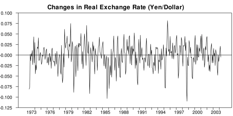
The distribution theory supporting the Dicker-Fuller tests assumes that the errors are statistically independent and have a constant variance. The changes of the real exchange rate are depicted as Figure 2, which strongly indicates that the sequence is serially correlated in that positive (negative) deviation persists for a rather period. Therefore, we should take some reservation about the power of the DF test.

t

[image:27.595.106.484.544.732.2]

q

Figure 2

Changes in Real Exchange Rate (Yen/Dollar)

1973 1976 1979 1982 1985 1988 1991 1994 1997 2000 2003 -0.125

-0.100 -0.075 -0.050 -0.025 -0.000 0.025 0.050 0.075 0.100

(28)

Phillips and Perron (1988) developed a test procedure that allows for the distribution of errors. The Phillips-Perron test (PP test) statistics are modifications of the DF t-statistics and the critical values are precisely the same.

The conclusion based on the PP test is the same as DF test; the γ statistics value is tested to be -2.3588, absolute value lesser than the 10 percent critical value( 2− .57).

From above we know that all kinds of unit root tests yield the same conclusion: we can not reject the null hypothesis of unit root in the process of real exchange rate q_t. Therefore, PPP does not seem to hold in the floating period.

Although PPP fails in this case, we can investigate further by testing relative PPP indicated by equation (3): *

t t

s p p_t

∆ = ∆ − ∆ . Thus, unit root test on the

“relative” real exchange rate is necessary since it becomes the error term in equation (3).

t

q

∆

*

t t t

q s p

[image:28.595.81.511.564.630.2]

∆ = ∆ − ∆ + ∆p_t (13) The test results can be summarized as Table 1 with γ denoting the coefficient of the first difference of ∆q_t₋₁ in unit root tests.

Table 1: Summary of the Unit Root Tests for ∆q_t

Test DF ADF PP t-statistics of γ -13.8278 -8.5079 -13.7641

Compare the t-statistics or γ with the DF test table to know that all exceed the 1 percent critical value(- . Therefore relative PPP seems to hold in the floating exchange rate period.

3.44)

(29)

3.1.3. Stationary process and UIP test

Recall the UIP theory * 1

( )

t t t t t

E s₊ − = −s i i and we know that to test UIP involves the estimation of future nominal exchange rates_t₊₁. In this paper we assume the perfect foresight, i.e. there is no expectation error: . Under this assumption, UIP becomes:

1 1

( )

t t t

E s₊ =s₊

*

t

i

1

t t

s₊ − = −s i_t . Then we use the following regression to test UIP:

1

t st it

ε = ∆ ₊ − ∆ (14) where ε_t is the UIP error term, ∆s_t₊₁=s_t₊₁−s_t and *

t t

i i i_t

∆ = − .26_{UIP holds}

if the error term ε_t is tested to be stationary. Like PPP test of equation (9), we are interested in whether γ =0 in the equation,

0 1

1

p

t t i t i

i

t

ε α γε₋ β ε₋ τ

=

∆ = + +

∑

+ (15)

where τ_t is the error term.

[image:29.595.61.531.603.666.2]

The test result can be summarized as the Table 2. Since all the absolute values of t-statistics are greater than that of the 1 percent critical value (-3.453), we can reject the null of unit root. Therefore we conclude that the error term in UIP, ε_tis stationary and UIP holds in the floating period.

Table 2: Summary of the Unit Root Test for UIP

Test DF ADF PP

t-statistic of γ -7.4504 -4.6556 -7.3324

Figure 3, 4 and 5 depict the nominal and real interest differential and the

26

and are both tested to be I(1) processes. 1

t

s₊

∆ ∆i_t

(30)

relative CPI changes between U.S and Japan in the floating period.

Figure 3

Nominal Interest DIfferential(Japan-U.S)

1978 1981 1984 1987 1990 1993 1996 1999 2002 -0.12

-0.10 -0.08 -0.06 -0.04 -0.02 0.00 0.02 0.04

[image:30.595.103.485.474.720.2]

Source: DataStream

Figure 4

Real Interest Differential(Japan-U.S)

1978 1981 1984 1987 1990 1993 1996 1999 2002 -0.075

-0.050 -0.025 0.000 0.025 0.050 0.075 0.100 0.125

(31)

[image:31.595.106.485.120.312.2]

Figure 5

CPI Index Change Differential(Japan-U.S)

1973 1976 1979 1982 1985 1988 1991 1994 1997 2000 2003 -4

-3 -2 -1 0 1

3.2. The Model of Exchange Rate Determination

3.2.1.

−

*

Is the relative price enough to determine the exchange rate?

The success of relative PPP may lead someone to believe that the price

differential is enough to explain the movement of the nominal exchange rate.

This section, however, argues that we should discard this optimistic idea.

Assume that only the price differential between Japan and U.S determines

the Japanese nominal exchange rate, then we can write out this as the following

order bivariate vector autoregressive (VAR) system in its standard form:

p-th

* *

10 1 1 1 1

1 1 1

( ) ( )

p p p

t m t m m t m m t m t

m m m

s a b s₋ c p p ₋ d i i e

= = =

= +

∑

+

∑

− +

∑

− + (15-1)

* *

20 2 2 2 2

1 1 1

( ) ( ) ( )

p p p

t m t m m t m m t m t

m m m

p p a b s₋ c p p ₋ d i i e

= = =

− = +

∑

+

∑

− +

∑

− ₋ + (15-2)

wheree₁_t, e₂_t are white-noise disturbances.

Equation (15) is called the restricted system in that all the coefficients of

(32)

interest differential, and are assumed to be zero. We will employ a block exogeneity test, which is useful for detecting whether to incorporate a variable into a VAR, to test whether the restriction is appropriate.

1m

d d₂_m

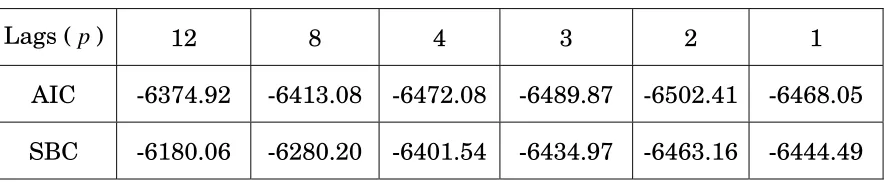
In empirical studies, we should determine the lag length p before performing the block exogeneity test. Here we use Akaike(1974) Information Criterion (AI ) and Schwartz (1978) Bayesian Criterion (SB ) criteria to aid in selecting the appropriate lag length:

C C

log | | 2

AIC=T

∑

+ N (16-1) log | | log( )

SBC=T

∑

+N T (16-2) where |

∑

|= determinant of the variance/covariance matrix of the residuals

= total number of parameters estimated in all equations.

N

Ideally, the AIC and SBC should be as small as possible (note that both can be negative). Under the assumption of both and to be zero, we calculate the values of the and based on different lags (Table 3). Apparently, Table 3 indicates that both AIC and SBC select the two lag model, i.e. .

1m

d d₂_m

AIC SBC

2

[image:32.595.78.520.545.636.2]

p=

Table 3: Summary of AIC and SBC Values in selecting lag P

Lags (p) 12 8 4 3 2 1

AIC -6374.92 -6413.08 -6472.08 -6489.87 -6502.41 -6468.05 SBC -6180.06 -6280.20 -6401.54 -6434.97 -6463.16 -6444.49

Let

∑

and be the variance/covariance matrices of the restricted and unrestricted systems, respectively, T represents the number of usable observations and let denote the maximum number of regressors contained in the longest equation. Asymptonically, as recommended by Sims (1980), the test

r

∑

u

c

(33)

statistics

(T−c)(log |

∑

_r| log |−

∑

_u|) (17) has a χ2_{distribution with degrees of freedom equal to the number of restrictions}

in the system.

If p= , the number of restrictions in equation (15) is 6 (lags 0,1,2 in each equation) and the statistics is calculated to be 50.6849, far exceeding the 1 percent critical value . The restriction is binding and therefore the interest differential is essential in the determination of the exchange rate.

2 (16.81)

3.2.2.

t p t i p

The model of exchange rate determination

From the previous work, we know that both the relative PPP

and UIP hold. Moreover, the interest rate differential should be included in the exchange rate determination besides the price differential. To derive the linkage between the PPP and UIP, we rewrite them as:

* t t s p ∆ = ∆ − ∆ * 1

t t t

s₊ − = −s i

*

t t t

s p p η

∆ = ∆ − ∆ + (18-1)

* 1

t t t t

s₊ − = − +s i i η_i (18-2) where η_p and η_i are the error terms. By differencing equation (18-2) we get:

*

1 ( )

t t t t

s+ s i i ηi

∆ − ∆ = ∆ − + ∆ (18-3) and by substituting (18-1) into the (18-3) we obtain:

* *

1 ( ) ( )

t t t t t

s₊ p p i i η

∆ = ∆ − + ∆ − + (19) where η η= _p+ ∆η_i.

Equation (19) is a model of nominal exchange rate determination; it can be interpreted that the increases in either price or the interest rate differentials will cause the future nominal exchange rate to depreciate. For example, if a country is suffering higher inflation or sharp interest rate increasing, its exchange rate

(34)

will depreciate according to equation (19). We can proceed to set a VAR system as:

* *

10 1 1 1 1

0 0 0

( ) ( )

p p p

t m t m m t m m t m t

m m m

s a b s₋ c p p ₋ d i i e

= = =

∆ = +

∑

∆ +

∑

∆ − +

∑

∆ − ₋ +

*

(20-1)

* ₂₀ ₂ ₂ * ₂ ₂

0 0 0

( ) ( ) ( )

p p p

m m m

p p a b s₋ c p p ₋ d i i e

= = = ∆ − = +

∑

∆ +

∑

∆ − +

∑

∆ − ₋ + * − (20-2) * *

30 3 3 3 3

0 0 0

( ) ( ) ( )

p p p

m m m

i i a b s₋ c p p ₋ d i i e

= = =

∆ − = +

∑

∆ +

∑

∆ − +

∑

∆ − + (20-3)

System (20) is not in the standard or reduced form in that it contains contemporaneous variables in two sides of the same equation. It is called

structural VAR since the model structure is based on the economic theory.

3.3. Econometric Analysis

3.3.1. Cointegration analysis

The same ordered variables are said to be cointegrated if there exist a linear combination that yields a stationary process. If the nominal exchange rate determination model described by equation (19) is appropriate, we can say that the three variables concerned are cointegrated:∆s_t₊₁, *

(pt pt)

∆ − and . We will use Engle-Granger methodology to test for the cointegration between them.

* (it it) ∆ −

The first step is to pretest the orders of integration. Cointegration necessitates that the variables be integrated of the same order. Various tests including Dicker-Fuller (DF), augmented Dicker-Fuller (ADF) and Phillips-Perron (PP) tests are used on the three variables in the model to reach

(35)

the conclusion that∆s_t₊₁, ∆(pt−pt*) and

* (it it)

∆ − are all I(0) processes27_.

The second step is to get the long run equilibrium relationship by regressing:

*

1 ( ) ( )

t p t t i t t

s₊ α β p p β i i* ε_t

[image:35.595.98.492.234.354.2]

∆ = + ∆ − ∆ + ∆ − ∆ + (21) where ε_t is the error term. The regression result is reported in Table 4.

Table 4: Estimation of the Exchange Rate Determination Model

coefficient value Std Error t−statistics significance

α -0.0034 0.0018 -1.87 0.0622

p

β -0.7465 0.3372 -2.2136 0.0276

i

β 0.1402 0.1950 0.7190 0.4727

Let /

t

ε denote the estimated error term from equation (21) to distinguish itself from the real error termsε_t . The residual of ε_t/ should be checked for unit roots to find whether it is stationary or not. If it is stationary, we can conclude that cointegration exists among∆s_t₊₁, ∆(pt− pt*) and

* (it it)

∆ − and vice versa. The following two equations are estimated:

/ /

1 1

t t e

ε α ε₋

∆ = + t

t

(22-1)

/ / /

1 1 1

t t i t i e

ε α ε₋ α₊ ε₋

∆ = +

∑

∆ + (22-2) where e_t are white noise.

It should be noted that we should not use the DF table because the residuals

/

t

ε in equation (22) are not the actual error terms. Only when we know the actual errors in each period can we use the DF table. Engle and Granger (1987) perform the set of Monte Carlo experiments to construct the confidence intervals

) 30 27 , 1 t

s₊ (pt −p*t and are all tested to be I (1) processes; their first difference are

all stationary.

(36)

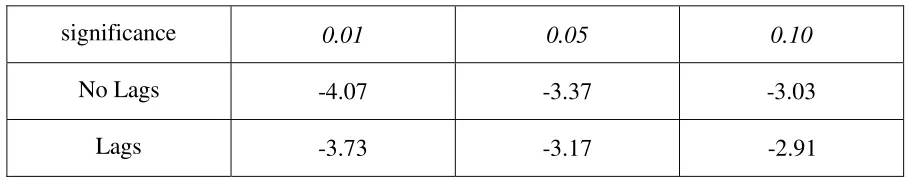
for α₁ in equation (22). Under the null hypothesisα₁=0, the critical values for the t-statistics depend on whether or not the lags are included (Table 528_).

7

[image:36.595.70.528.179.269.2]

( t − p

Table 5: Critical Values for the Null of No Cointegration

significance 0.01 0.05 0.10

No Lags -4.07 -3.3 -3.03

Lags -3.73 -3.1 -2.91

The estimated t-statistics of α₁ in (22.1) and (22.2) are –12.47557 and –7.9515, respectively, both exceeding the critical values for the null hypothesis of no cointegration at 1 percent level. Therefore, we can reject the null hypothesis of no cointegration and conclude that CHEER approach is supported in the short run.

3.3.2. The effect of the modification and the increased test power

It is worthy noting that the supportive evidence of CHEER approach is found according to equation (19), the first-order differenced model. In most of the recent CHEER papers, however, cointegration is directly searched between s_t₊₁,

*

t

p and ( . Here we will show that this modification is necessary because we can not find cointegration if using the same method as the recent papers.

*

t t

i −i

) )

Now we proceed to use Johansen methodology, the more powerful cointegration test, to investigate the cointetgration relationship betweens_t₊₁,

*

(pt − pt) and . Johansen methodology circumvents the small sample size

* (it −it )

28_{Table 5 is excerpted from Enders (1995).}

(37)

[image:37.595.66.527.220.353.2]

distortion problem and it can detect the multiple cointegration vectors. Further, the unnecessary step-by-step approach in Johansen methodology avoids any potential enlarged error from the previous step. The Johansen test results are summarized in Table 629_.

Table 6-1: Summary of the Johansen test betweens_t, (p_t − p_t*) and (i_t −i_t*)

Eigenv L-max Trace H0: r p-r L-max95 Trace95

0.0679 20.83 39.77 0 3 21.07 31.52

0.0483 14.66 18.95 1 2 14.90 17.95

0.0144 4.29 4.29 2 1 8.18 8.18

Table 6-2: Summary of the Johansen test betweens_t₊₁, (p_t −p_t*) and (i_t −i_t*)

0.0617 18.85 40.37 0 3 21.07 31.52

0.0562 17.11 21.52 1 2 14.90 17.95

0.0148 4.40 4.40 2 1 8.18 8.18

Table 6-3: Summary of the Johansen test between∆s_t₊₁,∆(p_t −p_t*)and ∆ −(i_t i_t*)

0.1487 47.51 87.52 0 3 21.07 31.52

0.0817 25.14 40.01 1 2 14.90 17.95

0.0492 14.88 14.88 2 1 8.18 8.18

Table 6-1 is the result of Johansen methodology based on the cointegration

29_{Source of the}

L-Max and L-Trace statistics: Enders (1996)

(38)

analysis between the contemporaneous exchange rate, price and interest rate differentials, which is the method adopted by most of the other researchers. Table 6-2 gives the cointegration analysis between the expected future exchange rate, price and interest rate differentials while Table 6-3 is the result of the modified model, i.e., the differenced model of equation (19). Comparing the results in the three sub-tables, we conclude that the effect of this modification is significant. Only Table 6-3, i.e., the sub-table with the modified model can yield the cointegration relationship30_.

3.3.3.

1t

e

The error correction model (ECM)

According to Granger representation theorem, cointegration and error correction are equivalent representations, i.e. cointegration implies error correction and vice versa. The next stage involves the error correction model for the VAR system (20), which should have the form of:

1 1 1 1

( st+ ) α β

∆ ∆ = + Φ + Π + (23-1)

∆∆ −(p p*)t =α₂+ Φ + Π +β₂ ₂ e2t

3t 1) t i₋ 3 (23-2) (23-3) *

3 3 3

(i i )t α β e

∆∆ − = + Φ + Π +

where Φ = ∆ − −st α βp(∆pt−₁− ∆pt*−₁)−βi(∆it−₁− ∆*

1

( ) ( )

n =

∑

βsn∆ ∆st+ +

∑

βpn∆ ∆ − ∆pt pt +

∑

i ∆ ∆

31_,

* *

( ), 1, 2,

n it it n

β

Π − ∆ =

1t

e , e₂_t and e₃_t =white-noise disturbances which may be correlated with each other and α , β are parameters.

represents the real error

Φ ε_t₋₁ in equation (21). Since ε_t/₋₁ is the

30

In Table 6-1 and Table 6-2, L-Max and L-Trace contradicts each other in that only the latter rejects cointegration. We should pin down the number of cointegration vectors and therefore we conclude that there is no cointegration.

31 p

β and βi are the cointegrationg vectors given by equation (21).

(39)

estimation of deviation from long-run equilibrium in period(t−1), as proposed by Engle and Granger, it is possible to use the saved residuals {εt/−₁}

1 1

obtained from the regression of equation (21) as an instrument for the expression . Based on this substitution, the error-correction model (ECM) is estimated to be:

Φ 1t t e t 2t / 1

( st+ ) 0.00013 0.76179εt− e

∆ ∆ = − − + Π + (24-1)

(-7.8129) (0.00000)

* /

1 2

(p p )t 0.012055εt−

∆∆ − = − + Π + 2 (24-2)

(-0.65688) (0.5118)

(24-3)

* /

1 3 (i i )t 0.0001 0.033εt− e

∆∆ − = + + Π + ₃

(1.02725) (0.3052)

The value in the parenthesis under each equation shows t-value and the significance level. In equation (24.1), the error-correction term is of highly significance level. This suggests that the future change of exchange rate is strongly determined by the long-run equilibrium. Further, the sign of the error-correction terms ε_t₋₁ in equation (24.2) is not consistent with the theory, making (24.2) looks more like error-amplifying rather than error-correction. The significance level, however, is very low. This indicates that the differenced price level is rather rigid and does not respond to the deviation from the long-run equilibrium level much.

3.3.4. Causality test and innovation accounting

In VAR analysis, we say that does not Granger-cause q if the lagged values of do not appear in the equation for , that is, the current and lagged do not help to predict the future value of . The null hypothesis that does not Granger-cause can be tested by doing a joint F-test: regress on both the lagged and the lagged and see the significance of the coefficient of lagged .

1t q 1t q t 2t

q q₁_t

1t

q

2t

q q₁_t

2t

q q₂_t

1

q q₂_t

(40)

The following part of this section investigates the Granger causality relationship among the three variables in the exchange rate determination model: ∆s_t₊₁ ,

* (pt pt)

∆ − and ∆ −(it it* while performing the innovation accounting.

∆ )

[image:40.595.69.528.266.386.2]

Based on the VAR system (20), we first conduct the Granger causality test. The F-test and the corresponding significance level are reported in Table 7.

Table 7: Summary of Granger-Causality Tests

variable st+1

* (p_t p_t)

∆ − *

(i_t i_t) ∆ −

1

t

s₊

∆ 21.57 0.000 0.024 0.976 0.722 0.487

4.121 0.017 7.184 0.001 5.234 0.006 *

(it it)

∆ − 1.741 0.177 0.361 0.697 2.622 0.074 *

(pt pt)

[image:40.595.70.530.267.387.2]

∆ −

Table 7 shows that ∆s_t₊₁ Granger-causes only itself; ∆ −(it it*) also roughly

Granger-causes only itself, while ∆(pt− pt*) Granger-causes all the three variables.

To further identify the different roles ∆(pt −p*t) and

* (it it)

∆ − play in the model of exchange rate determination, we can decompose the forecast error variance. The forecast error variance decomposition tells us the proportion of the movements in a sequence due to its own shocks versus shocks to the other variables.

We use the variance matrix in the VAR system (20) to obtain 1-step ahead through 24-step ahead forecast errors. Appendix 4 shows the first five impulses, together with the variance decomposition. To measure all responses in terms of standard deviations, we depict the following impulse response functions.

(41)

[image:41.595.120.475.111.654.2]

Figure 6-1

Plot of Responses To ds

0 2 4 6 8 10 12 14 16 18 20 22

-0.2 0.0 0.2 0.4 0.6 0.8 1.0

ds ddp ddi

Figure 6-2

Plot of Responses To ddp

0 2 4 6 8 10 12 14 16 18 20 22

-0.25 0.00 0.25 0.50 0.75 1.00

ds ddp ddi

[image:41.595.124.481.125.347.2]

(42)

[image:42.595.116.473.122.350.2]

Figure 6-3

Plot of Responses To ddi

0 2 4 6 8 10 12 14 16 18 20 22

-0.2 0.0 0.2 0.4 0.6 0.8 1.0

ds ddp ddi

Note: ds = ∆st+₁,ddp= ∆(pt − pt*)and

* (t t )

ddi= ∆ −i i .

From the Granger causality test and innovation accounting analysis, we can see that the price differential itself can not explain all the movements of the future nominal exchange rate. ∆(pt−pt*)

)

t

s

explains only 0.011 percent of the movement of while explains 0.34 percent in the 5-lag (five month) ahead horizon. The differenced interest rate differential serves as a “channel” in the sense that it does not Granger cause

1

t

s₊

∆ *

(it it

∆ −

1

+

∆ directly but it explains more of the movement of the exchange rate. Some of the effects of ∆(pt−pt*)on ∆st+1are

conveyed by this “channel”: ∆(pt−pt*) affects

* (it it)

∆ − and then affects the nominal exchange rate movement.

* (it

∆ −it)

The exchange rate determination model is derived from the economic theories and the differenced variables make it a little difficult to grasp the real effects since differencing tends to smooth the various shocks. Moving away the

International Parities and Exchange Rate Determination

Munich Personal RePEc Archive

International Parities and Exchange Rate

Determination

Zhao, Yan

31 March 2005

International Parities

and

Exchange Rate Determination

Yan Zhao

Abstract

Acknowledgements

Contents

1.

Introduction

1.1.

PPP as the First Exchange Rate Model

1.2.

Combining PPP with UIP (CHEER)

1.3.

Two Problems of the CHEER Approach

1.4.

Solution of the Two Problems

2.

Literature Survey

2.1

Review of PPP

2.1.1.

What’s PPP?

2.1.2.

Empirical tests of PPP

2.2

Review of UIP

2.2.1.

What’s UIP?

2.2.2.

Empirical test of UIP

2.3

Cointegration Analysis of PPP and UIP

3.

Short-Run Analysis (Jan. 1973~Jun. 2004)

3.1.

Pretests of PPP and UIP

3.1.1.

Unit root process and Dickey-Fuller test

∑

3.1.2.

Nonstationary process and PPP test

3.1.2-1

The DF test

3.1.2-2 The Augmented DF test

∑

∑

∑

3.1.2-3 The Phillips-Perron Tests

3.1.3.

Stationary process and UIP test

∑

3.2.

The Model of Exchange Rate Determination

3.2.1.

Is the relative price enough to determine the exchange rate?

∑

∑

∑

∑

∑

∑

∑

∑

∑

∑

∑

∑

∑

3.2.2.

The model of exchange rate determination

∑

∑

∑