Endogenous Comparative Advantage

Munich Personal RePEc Archive

Endogenous Comparative Advantage

Moro, Andrea and Norman, Peter

Vanderbilt University, University of North Carolina - Chapel Hill

1 March 2005

Endogenous Comparative Advantage

Andrea Moro§ _{Peter Norman}¶

February 8, 2018

Abstract

We develop a model of trade between identical countries. Workers endogenously acquire skills that are imperfectly observed by firms, who therefore use aggregate coun-try investment as the prior when evaluating workers. This creates an informational externality interacting with general equilibrium effects on each country’s skill premium. Asymmetric equilibria with comparative advantages exist even when there is a unique equilibrium under autarky. Symmetric, no-trade equilibria may be unstable under free trade. Welfare effects are ambiguous: trade may be Pareto improving even if it leads to an equilibrium with rich and poor countries, with no special advantage to country size.

Keywords: Comparative Advantage, Specialization, Human Capital.

JEL Classification Number: D62, D82, F11, O12

∗_{It is nearly impossible to thank everybody that contributed comments and suggestions. We thank them}

all. Special thanks to Lutz Hendricks, Pat Kehoe, Tim Kehoe, Narayana Kocherlakota, John Knowles, Rody Manuelli, Andrew Postlewaite, Paul Segerstrom, Ananth Seshadri, Robert Staiger, Kjetil Storesletten, Scott Taylor and Fabrizio Zilibotti for helpful comments, suggestions and discussions. We also thank the editor, the anonymous associate editor, and two anonymous referees for their comments. Support from NSF Grants #SES-0003520 and #SES-0001717 is gratefully acknowledged. The research for this paper was done partly when Peter Norman was visiting IIES Stockholm and he is grateful for their hospitality.

§_{Department of Economics, Vanderbilt University. Email:}

[email protected]

¶_{Department of Economics, University of North Carolina at Chapel Hill. Email:}

I

Introduction

In this paper we develop a stylized model of international trade in which a country can establish a reputation for having a high quality labor force, providing new insights to the understanding of the causes of trade, specialization, and inequality across countries.

A reputation for high or low quality of the labor force may arise when employers do not perfectly observe workers’ competencies and skills. Workers acquire human capital not only through education and labor market experience, but also with personal effort and investments that are not as easily observable. Our paper focuses on this informational asymmetry, showing that it may generate reputational differences across countries that are self-fulfilling.

The labor economics literature has shown that informational asymmetries of this kind are empirically relevant. Farber and Gibbons (1996) and Altonji and Pierret (2001) first showed that employers’ learning is significant, providing support to the assumption that employers initially observe workers’ skills with noise.1 Recent literature confirms these results2 _{suggesting a significant scope for the mechanism proposed in this paper to play}

a role in determining workers’ wage distribution, incentives to acquire skills, and sorting across industries.

Based on this evidence, one cannot dismiss the possibility that labor market informa-tional asymmetries may also play a role in explaining, at least in part, trade and special-ization across countries. In this paper, we demonstrate that they are sufficient to generate self-fulfilling cross-country differences in reputation that imply human capital differences, trade, and specialization between otherwise identical countries. There is arguably an incom-plete understanding of the patterns of trade and specialization observed in the real world, which suggests that exploring alternative models could provide new insights.3

In our model, technology has constant returns to scale, a country is defined as a labor market, and international trade is frictionless. Countries are symmetric in every respect,

1_{In most of the literature, the identification of the main effect exploits panel data where workers are}

observed over time. If employers imperfectly observe workers’ skills, but learn over time through the obser-vation of productivity signals, then as tenure increases wages should become more correlated with measures of productivity available to the researcher (typically, workers’ scores in aptitude tests).

2_{In particular, Lange(2007) measured the “speed” of employer learning finding that, according to the}

best estimates, it takes three years for an employer to reduce her expectation error to 50 percent of its initial value, and 26 years to reduce it to less than 10 percent of its initial value. Note that average employer tenure is currently just above 4 years on average, (January 2016, see the U.S. Bureau of Labor Statistics news release “Employee Tenure”, https://www.bls.gov/news.release/tenure.toc.htm, last accessed: August 2, 2017). See also Sch¨onberg (2007), Pinkston(2009), and Kahn and Lange (2014) using U.S. data, and

Lesner(2017) with Danish data. Cornwell et al.(2017) use Brazilian data to show that employer variation in workers’ perceived race significantly affects wages.

3_{A full empirical investigation of the model implications, which would require accounting for (and}

therefore the model always admits symmetric equilibria that replicate autarky, without gainful trade. The only aspect of the model that is non-standard is workers’ skill acquisition. Our main questions are whether there exist conditions under which there also are equilibria with asymmetric country reputations for skill investments and what are the properties of such equilibria.

Workers can acquire skills at a cost that varies across workers. There are two sectors de-manding labor, a “high tech” sector and a “low tech” sector, and skills increase productivity only in the high tech sector. Incentives to acquire skills are affected by an informational asymmetry: workers’ skills are only observed by employers with noise, through a signal of productivity that may be thought of as aggregating information provided by the worker’s curriculum, interviews, and observation in the workplace. A worker without skills, which we henceforth call anunqualified worker, may send a good signal, but this is less likely than a qualified worker (a worker with skills) sending a good signal.

Before observing the noisy signal, the prior probability of investment is determined in each country by aggregate investment rates summarized by the proportion of qualified workers. The probability of investment of each worker is then computed using her signal, but is also affected by the prior. Hence, the actual proportion of qualified workers, together with endogenous relative prices, determines incentives to invest. There is no point in investing in skills if there are very few qualified workers in the country because firms will interpret a good signal as most likely being noise and the good signal will raise the wage very little. Symmetrically, if almost all workers invest, firms will ignore bad signals as “bad luck”, and, again, there is no point in investing since all workers get high wages regardless of the signal. Incentives to invest are therefore at the highest at some intermediate level of aggregate investment because this is when firms will pay most attention to the noisy signals.

Hence, starting from a relatively low level of investments, the value to acquire human capital will increase if the proportion of skilled workers in the economy increases as the signal to noise ratio decreases. Working against this there are relative price effects that make the high tech good less valuable when its supply increases, but these effects are smaller when countries trade than in autarky. Additionally, when skills increase in one country, the incentives to acquire skills in the other country are unambiguously reduced because of the price effects. Hence, an asymmetric allocation of human capital and goods production may arise even if there are no fundamental differences between the countries. As far as we know, this is an explanation of trade and specialization that is novel in the international trade literature. What is crucial for this result is that the reputation for having a qualified labor force is like a public good, operating within a country regardless of its size.

Scale economies and network effects can also create asymmetries between countries. How-ever, these models usually start with some exogenous differences that are being accentuated in equilibrium. Moreover, in existing models it is typically an advantage to have a large domestic market, whereas in our model there is no systematic effect favoring large countries. It is not the number, but the proportion of qualified workers that is critical in generating the reputational externality. This is because employers, when assessing workers, use the proportion of qualified worker as their prior for human capital investment. A worker is more likely to be qualified the higher the proportion of qualified workers there are in her country.

We highlight this irrelevance of country size by showing that there is no systematic advantage to large economies. In many parameterizations where country sizes are allowed to differ, there is an equilibrium with the large country specializing in the high tech industry as well as an equilibrium in which the small country is the richer. Which of these equilibria leads to more inequality or higher welfare is also a matter of parameter choices.

Asymmetric equilibria arise under free trade, but as already noted, there is always at least one symmetric equilibrium with no gainful trade that replicates the autarky allocation. One may therefore ask whether coordinating on an asymmetric equilibrium is plausible, and several properties of our model suggest that it may be.4 First, this isnot a model in which certain countries are trapped in a coordination failure and others are not. Incentives in one country depend on investments in the other and relative price effects are a crucial component in the model. Asymmetric equilibria may therefore occur even if the autarky equilibrium is unique. Moreover, the stability conditions under autarky differ from the stability conditions under free trade. Opening up international trade may destabilize the unique and stable autarky equilibrium, so cross country income differences may be an inevitable aspect of free trade even if there are no exogenous differences that “explain” which country becomes richer.

In any asymmetric equilibrium, a country with more human capital is richer and better off than the other country. However, this does not necessarily imply that the poor country is worse off under trade than in autarky. Welfare in the poor country can go either way, but we emphasize the less intuitive possibility by generating an example where an asymmetric equilibrium Pareto dominates the autarky equilibrium. The intuition is that an increase in the skill level abroad may drive down the relative price of the high-tech good so much that exchanging the low-tech good for the high-tech good generates higher welfare in the poor country compared to domestic production.

4_{Matsuyama (2002) argues that multiplicity by itself does not offer a compelling reason for observed}

Our results are robust to introducing exogenous productivity differences. If one country has a “fundamental” comparative advantage in the high-tech industry, it may still special-ize as a low-tech industry as a result of the mechanism in our model, provided that the exogenous differences are not too large.

The rest of the paper is structured as follows. The next section discusses the contribution of this paper relative to existing literature. Section III introduces the model, defines the equilibrium, and shows that it can be characterized as a planner’s problem, simplifying the analysis that follows. Section IV characterizes the equilibria under autarky. The main result, the existence of equilibria with trade and specialization, is presented in Section

V. Section VI discusses the stability and welfare properties of equilibria with trade, and the irrelevance of size. Section VII concludes discussing the robustness of the results to extending the model to multiple countries, to including physical capital in the production, and migration.

II

Related literature

Our main contribution to the literature is to suggest a novel source of trade and compara-tive advantage between identical countries. There are several papers in the literature that include some of the crucial elements of our model, imperfectly observed human capital accu-mulation, but in those models either some exogenous differences are posited, or equilibrium multiplicity in a baseline autarky model is the driving source of specialization.

Our model relates to a literature on trade and endogenous skill formation initiated by

Findlay and Kierzkowski(1983), who develop a general equilibrium model where the driver of trade is endogenous human capital acquisition. As in our model, the factors of production are skilled and unskilled labor, but countries specialize because of exogenous differences in the availability of inputs needed to acquire human capital, generating what we refer to as price effects. In our setup instead, countries are identical also in the cost of acquiring human capital.5

Among the papers presenting models with asymmetric information, Grossman and Maggi(2000) andGrossman(2004) have elements that are similar to our setup: a Hecksher-Ohlin model with imperfectly observable skills. Their focus is on comparative statics with respect to changes in the skill distribution. For their purposes it is sufficient to consider

5_{The focus of this literature is mainly in showing how even if factor price equalization holds (for the}

marginal worker), trade induces different incentives to acquire human capital across countries. For recent extensions see alsoRanjan(2001),Falvey et al.(2010),Auer(2015),Unel(2015),Blanchard and Willmann

(2016), and Danziger(2017). In some cases, the exogenous country differences are assumed by analyzing the effects of trade on a small open economy that takes the world price as given, as in Cartiglia (1997),

how trade is affected by exogenous differences in the talent distribution across countries, therefore they ignore the incentives to acquire skills that are central in our model.6

Costinot (2009), like us, seeks to formulate a more fundamental theory of comparative advantage. The technology is also based on the idea that human capital is more important for some firms than for others. The main difference is that the model ultimately derives cross country differences from exogenous differences in institutional quality and human capital.

Chisik (2003) derives trade in a model where products may acquire, in equilibrium, different reputation for quality. Self-fulfilling reputation determines the average quality of a country exports, and comparative advantages arise endogenously because countries coordinate on selecting different equilibria.7 Similarly, in Chatterjee (2017) comparative advantages emerge endogenously as a Nash equilibrium of a game in which countries choose policies that affect sector-specific productivities or relative factor endowments. In these papers equilibrium multiplicity is needed to generate the comparative advantage. In our model instead, trade may arise even when there is a unique autarky equilibrium.

While our underlying assumptions are very different, our model shares many features with trade models with increasing returns (Ethier(1982), Krugman(1980)), their versions usually referred to as “agglomeration models” (Krugman and Venables (1995), Puga and Venables (1999)), and the “symmetry-breaking” literature (see Matsuyama (1996, 2004)). Agglomeration models can sustain a concentration of (high-income) manufacturing because production costs decrease with the size of the industry. Manufactured goods are inputs in the production of other goods, implying that being close to other producers saves on trans-portation costs. This creates incentives to concentrate production. When production costs are neither too small nor too large, there are equilibria where manufacturing is concentrated in one country that becomes richer.

While our model is considerably less complicated and closer to the neoclassical bench-mark than models with increasing returns, there is a close similarity in how a pecuniary

6_{A number of papers study the effects various informational asymmetries on trade. Their focus is}

essen-tially on analyzing the effects of asymmetric information and not on studying how trade arises in equilibrium.

Vogel(2007), focuses on the effect of institutional quality reducing workers’ moral hazard. Davidson and Sly(2014), focus on how opening to trade affects one country’s distortions in human capital accumulations when education has a signaling role. Park(2011) analyzes trade agreements under imperfect public moni-toring,Zhang(2012) consider effects of asymmetric information when exporters are credit constrained, and

Creane and Jeitschko(2016) show that weak institutions may result in welfare-reducing trade in an adverse selection model. Razin and Sadka(2003) use an informational asymmetry to model the role of foreign direct investments, Casella and Rauch (2002) derive a role for minority groups in international trade using an informational friction, andMcCalman(2002) considers the impact of asymmetric information in bargaining about trade agreements. Eicher(1999) considers a model that is significantly richer than ours in many ways, but the informational asymmetry is modeled in reduced form.

7_{Other models based on trust and endogenous quality reputation areAraujo and Ornelas(2007),Araujo}

externality interacts with local market conditions. However, there are also crucial differ-ences: our model resorts to imperfect information rather than global increasing returns. Agglomeration models predict a positive relation between size and development whereas our model has no such implications, as illustrated in Section . This is because what matters in determining a country’s reputation is the proportion, not the number of skilled workers. We borrow some of the modeling assumptions from the statistical discrimination liter-ature. In Moro and Norman (2004) racial differences arise in a statistical discrimination model because groups specialize in the level of acquired skill. Here, countries take the role of racial groups, but embedding the reputational effects in a model in which spillover effects are carried by equilibrium price effects creates some additional complications that are ab-sent inMoro and Norman(2004). To make the analysis more transparent we have therefore simplified the information technology (the noisy signal has support on two realizations), the production technology (it is linear), so complementarities arise here because of convexity in consumer preferences only. All these simplifications can be relaxed at the cost of some additional complexity of the analysis.

III

The Model

Two countries, labeled by j=h, f,are populated by a continuum of agents, whereλh _and λf _{= 1−λ}h _{denote the mass of agents in each country. Agents are price takers. We build on} a simple 2×2×2 trade model but with factors of production being workers with and without human capital. The model is closed by a stylized model of human capital acquisition and an informational technology borrowed from the statistical discrimination literature.8 Workers cannot migrate.

All agents can invest in human capital by paying an investment cost c drawn from a cumulative density G defined on the interval [c, c]. Investment is binary, the investment costcis private information and is independent of which country the agent lives in. We call workers who invest in human capital qualified and the others unqualified. Agents have the same preferences. The utility of an agent consuming the bundle (x1, x2) isu(x1, x2)−cif the

agent invests andu(x1, x2) otherwise, whereu is a homothetic and strictly quasi-concave.

After the investments, nature assigns each worker a signal θ ∈ {g, b} that employers observe. For simplicity we assume that

Pr [g|worker qualified] = Pr [b|worker unqualified] =η > 1

2, (1)

where the restriction that η > 1/2 labels signals so that g is good news. Our preferred interpretation is that the unobservable investment is a costly effort decision and the signal is an imperfect measure of the costly effort, aggregating information from letter of recom-mendation, grades, tests, etc. . . .

The two consumption goods are produced solely from qualified and unqualified labor, denoted q and nrespectively, according to

y1(q, n) =q; y2(q, n) =q+n. (2)

All workers are thus perfect substitutes in industry 2,whereas only qualified workers con-tribute to the production of good 1.9

After defining equilibrium, we show in Subsection that given human capital investment the equilibrium in the goods and labor markets can be characterized as the solution to a planners’ problem, simplifying the derivations that follow. Section shows how technology can be represented graphically by a production possibilities set.

Equilibrium

Our notion of equilibrium is analogous to a competitive equilibrium in a perfect information environment, but the informational asymmetry makes the treatment of the “labor supply” somewhat non-standard: skilled labor is endogenously determined by incentives that depend on prices derived from the goods markets.

Consider an agent with realized wage w deciding how to allocate her earnings between the two goods given prices p= (p1, p2). The (ex-post) maximized utility of the worker is

v(w, p) = max x1,x2

u(x1, x2) (3)

subject to p1x1+p2x2 ≤w.

By strict quasi-concavity ofu(x1, x2), the optimization problem in (3) has a unique solution,

and, with the usual notational abuse, we denote the demand functions byx1(w, p), x2(w, p).

Employers cannot observe if a worker is qualified, so a labor demand is a map l :

{g, b} → R+. Denote with π any fraction of qualified workers in a country. This fraction

can be thought of as the prior probability of a worker being qualified, before employers observes the signal. Employers then use Bayes’ rule to form the posterior probability that

9_{This extreme technology is for simplicity only. In previous versions we considered a more general}

a worker is qualified given her signal:

µ(g, π)≡ ηπ

ηπ+ (1−η) (1−π) µ(b, π)≡

(1−η)π

(1−η)π+η(1−π). (4)

Associated with any fraction of qualified workers, π, and a given labor demand l, the corresponding quantities of qualified and unqualified workers are:

q = l(g)µ(g, π) +l(b)µ(b, π) (5)

n = l(g) (1−µ(g, π)) +l(b) (1−µ(b, π)),

We assume that a strong law of large numbers applies and treat q and n in (5) as both expected and realized inputs of labor.

Without loss of generality there is a representative firm in each sector and each country, which takes a wage schedule wj _{:{g, b} →R}

+ and output pricespi as given.10 Using the production function (2) and (5), the profit maximization problem for a Sector 1 firm is

max

l p1 l(g)µ g, π

j_{+l(b)µ b, π}j_−wj

gl(g)−w j

bl(b), (6)

For Sector 2, where qualified and unqualified workers are equally productive, the profit maximization problem is

max

l p2(l(g) +l(b))−w j

gl(g)−w j

bl(b). (7)

Agents have rational expectations about the wages and prices, but face uncertainty about the realization of the signal. Denotingv(w, p) the indirect utility function defined in (3), the expected utility for an agent in countryj with investment cost c is

ηv(wj_g, p) + (1−η)v(wj_b, p)−c (8)

if a worker invest in human capital, and

(1−η)v(wgj, p) +ηv(w j

b, p) (9)

if not. The worker is better off investing if and only if (8) exceeds (9), or if the cost of investment is less than the gross incentives: c≤ (2η−1)·(v(wgj, p) -v(wj_b, p)).The implied

10_{The caveat is that the informational asymmetry would disappear if (qualified) workers could start their}

proportion of investors in countryj is thus

πj =G(2η−1) (v(w_gj, p)−v(w_bj, p)). (10)

To sum up: optimal consumption plans are defined in (3), (6) and (7) describe the profit maximization problems for each sector, and (10) summarizes the individually optimal hu-man capital investments.

What remains to describe are the market clearing conditions. Factor market clearing requires that the aggregate demand for workers with each signal equals the mass of agents who draw the signal. That is, let l_ij = (l_ij(g), lj_i (b)) be a labor demand scheme in industry

iand country j and write the labor market clearing conditions as

lj₁(g) +lj₂(g) = ηπj+ (1−η) (1−πj) (11)

lj₁(b) +l₂j(b) = (1−η)πj+η(1−πj).

Finally, for the product market equilibrium conditions it is convenient to let xj_i be the output in industry iand country j. That is

xj₁ = lj₁(g)µ g, πj+l₁j(b)µ b, πj (12)

xj₂ = lj₂(g) +lj₂(b),

which allows us to write the product market clearing conditions for the world market as

X

j=h,f λj

   x

j i −

ηπj + (1−η) (1−πj)

| {z }

#agents with wagewjg

xi(wgj, p)−

(1−η)πj+η(1−πj)

| {z }

#agents with wagewj_b

xi(w_bj, p)

   = 0

(13) Our definition of equilibrium is then:

Definition 1 A competitive equilibrium consists of output prices p∗_{, wages w}j∗_{, labor}

de-mandsl_ij∗, outputsxj∗_i , and fractions of qualified workersπj∗ _{for each country j=h, f and}

industry i= 1,2 , satisfying:

(a) lj∗₁ solves (6) and lj∗₂ solves (7) given pi = p∗_i and xj∗₁ and xj∗₂ are the associated

profit maximizing outputs in j=h, f

We refer to a situation where all equilibrium conditions except the optimal investment condition (d) are fulfilled as a continuation equilibrium.11

A Planning Characterization of Continuation Equilibria

From the point of view of an informationally unconstrained planner, a continuation equi-librium is inefficient: qualified and unqualified workers with the same signal are treated symmetrically, resulting in a misallocation of workers to jobs. However, if the symmet-ric treatment of workers with the same signal is viewed as a fundamental property of the environment, then the equilibrium allocation is (constrained) efficientconditional on the in-vestment behavior. This allows us to describe aggregate equilibrium allocations as solutions to the planning problem:

max

(x1,x2)∈XW(πh,πf)

u(x1, x2), (14)

whereXW _πh_{, π}f _{is the world production possibilities set defined in Section .}

The following proposition shows that, forfixed investments, versions of the welfare the-orems hold: the equilibrium is characterized by a planning problem where the informational asymmetry is built into the feasible set. This allows us to appeal to simple graphs in the analysis that follows.

Proposition 1 Suppose that u(x1, x1) is homothetic. Then:

1. The aggregate world consumption in any continuation equilibrium is a solution to (14)

2. Suppose that (x∗

1, x∗2) solves (14), (p∗1, p∗2) is a normal to a hyperplane that separates the set of bundles such that u(x1, x2)≥u(x∗1, x∗2) and XW πh, πf

,and that wj∗g = maxp∗

1µ g, πj

, p∗

2 andw

j∗

b = max

p∗

1µ b, πj

, p∗

2 in each country j. Then these prices, wages and aggregate consumption are part of a continuation equilibrium.12

Proposition1immediately implies that, given any πh_{, π}f_{there is a unique continuation} equilibrium up to a re-normalization of the prices.

The Production Possibilities Set

A useful way to represent technology is in terms of the production possibilities set. The set of feasible production plans in a country depends on the fraction of workers that invest

11_{This term is mainly due to lack of a better alternative. Due to the workers being non-atomic it does}

not make a difference whether investments are made before or simultaneously with the wage posting.

12_{The allocation of workers in each country is somewhat complicated to describe in general, but is implicitly}

✲ ✻

✑ ✑ ✰

✑ ✑ ✰

dx₂ dx₁ =−

πη+(1−π)(1−η)

πη

dx2 dx₁ =−

π(1−η)+(1−π)η

π(1−η)

πη π

π(1−η) + (1−π)η

x1

x2

1

Figure 1: Per capita production possibilities in a country

in human capital, π. Figure 1 illustrates the (per capita) production possibilities set in a country, which we denote withX(π).

To understand the figure, first observe that (x1, x2) = (0,1) if all workers are producing

good 2, and that (x1, x2) = (π,0) if all workers are producing good 1, because only a fraction

π of the workers are productive in Sector 1. There are πη+ (1−π) (1−η) workers with signalg andπ(1−η) + (1−π)η workers with signal b.If all signalg workers are in Sector 1 (πη of these workers are productive) and all signal-b workers are in Sector 2, then the outputs are given by the point at the kink in the graph. The frontier to the right of the kink is steeper because in that region all g workers are employed in Sector 1, therefore to increase production firms must employ more b workers, who are less likely to be qualified. To the left of the kink instead, onlyg workers are employed in Sector 1.

The world production possibilities set is given byXW πh, πf=λhX πh+λfX πf

and is convex by convexity of X(π). The next proposition immediately follows, since the production possibilities set becomes (weakly) flatter as investment in any country increases:

Proposition 2 Suppose thatu(x1, x1)is homothetic. Then in any continuation equilibrium the relative price of the high-tech good is (weakly) decreasing in the countries’ investment

πh _{and π}f_.

IV

A Parametric Specification

xα

1x12−α, which imply demand functions:

x1(p, w) =

αw p1

x2(p, w) =

(1−α)w p2

. (15)

The continuation utility for a worker that earns wagew is therefore:

v(w, p) = α

α_(1−α)1−α pα

1p1

−α

2

w. (16)

We normalize settingp2= 1 and, with abuse of notation, writep(π), w_gj(π) and wj

b(π) for the unique continuation equilibrium prices and wages in good 2 units, whereπ= πh, πf.

A qualified worker earns wjg(π) with probability η and wj

b(π) with probability 1−η. Symmetrically, an unqualified worker earns wjg(π) with probability 1−η and wj

b(π) with probability η.Computing the expectation ofv(w, p) in (16) conditional on investment and subtracting from this the expectation of v(w, p) conditional on not investing we get the

gross benefits of investment for an agent in countryj,denoted Bj(π),which is given by

Bj(π) = E{v(w, p)|qualified} −E{v(w, p)|unqualified} (17)

= αα(1−α)1−α(2η−1)(w j

g(π)−wj

b(π)) (p(π))α .

Using condition (d) in Definition1we see that anyπsuch thatπj =G Bj(π)forj=h, f

gives an equilibrium fraction of investors in each country. All that remains to calculate full equilibria is to derive expressions for the continuation equilibrium prices.

Continuation Equilibria in Autarky

As a benchmark, we first consider a closed economy. Suppressing the country index, we write

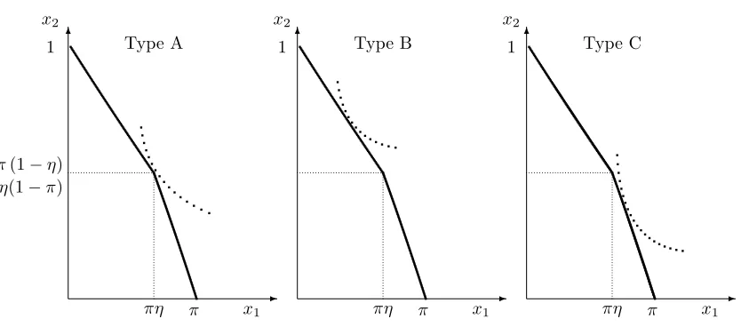
π for the proportion of qualified workers. There are three possible types of continuation equilibria, illustrated in Figure 2.13

Type A equilibria (allocation of workers “according to signals”). Graphically, this type occurs when the tangency is at the kink of the feasible set. That is, all workers with signal b (g) are working in the low (high) tech sector. Outputs are then x1 =ηπ and

13_{This is a somewhat unfortunate aspect of having only 2 signals. With a continuum of signals we would}

✻

x2

1 ✻

πη π x1

x2

1 ✻_❏

❏ ❏

❏ ❏

❏ ❏❏

❇ ❇

❇ ❇

❇ ❇

❇❇

x2

1

✲

πη π x1

✲

πη π x1

✲

Type A Type B Type C

π(1−η) +η(1−π)

Figure 2: Three types of continuation equilibria

x2 = (1−η)π+η(1−π),so the demands in (15) pin down the price of the high-tech good

as

p(π) = α 1−α

(1−η)π+η(1−π)

ηπ . (18)

Candidate equilibrium wages are obtained by the zero profits condition. Since p2 = 1, this

immediately gives wb(π) = 1. The high-tech firm sells ηπ units at price p(π) and hires ηπ+ (1−η) (1−π) workers with signal g. Zero profits in Sector 1 therefore implies that the wage in that sector, wg(π), equals the price of good 1 times the expected probability that a worker with signalg is productive in that sector µ(g, π):

wg(π) =p(π)µ(g, π) =p(π)

πη

πη+ (1−η) (1−π), (19)

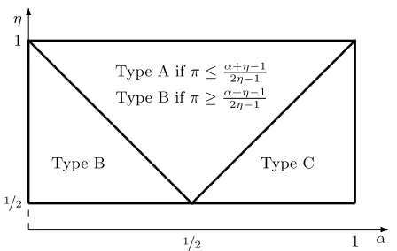
which has the alternative interpretation that the wage equals the expected value of output. Finally, we have to check that a high-tech firm has no incentive to hire signalbworkers, and that a low-tech firm has no incentive to hire signalg workers. These conditions give rise to inequalities that determine the region where a Type A equilibrium exists (see Figure 3).

η

1

1_/2 1_/2

1

α Type C

Type A ifπ≤α₂+ηη−−11

Type B ifπ≥ α₂+_ηη₋−₁1

Type B

✲ ✻

Figure 3: Types of autarky equilibria in the (α, η) space

Type C equilibria (mixing of bad signals). This equilibrium occurs when the demand for the high-tech good is strong (i.e. when the Cobb-Douglas share of good 1 parameterα

is high). In Figure 2, this corresponds to a tangency to the right of the kink. In this case a fraction β of workers with signal b(defined below) works in Sector 1. Workers with signal

bemployed in the low-tech sector are paid 1. Signal-bworkers in the high tech sector must be paid their expected productivity, which equals the price times their probability of being productive, orp(π)·µ(b, π). But sinceb-signal workers must be paid the same wage in both sectors,wb(π) =p(π)·µ(b, π) = 1 we can pin down the price of good 1 as the inverse of the probability that a bad signal worker is productive in the high-tech sector,

p(π) = 1

µ(b, π) =

π(1−η) + (1−π)η

π(1−η) (20)

The price must also satisfy a relationship imposed by demand shares (15):

p(π) = α 1−α

x2produced byb-workers

z }| {

(1−β) ((1−η)π+η(1−π))

ηπ

|{z}

x1produced bygworkers

+ β(1−η)π

| {z }

x1produced bybworkers

(21)

Equating the right-hand sides of (20) and (21) determines the fraction ofb-signal workers employed in Sector 1, β.The solution reveals that a positive β exists if and only if α > η,

as illustrated in Figure3. We refer the reader again to the web appendix for details.

Equilibrium investments in Autarky

Figure 4: Gross incentives to invest under autarky

as:14

B(π) = max

(2η−1)

πη

π(1−η) + (1−π)η

α

α−(πη+ (1−π)(1−η))

πη+ (1−π)(1−η)

,0

. (22)

Figure 4plotsB(π) for two sets of parameter values. All values whereB(π)>0 in the figure correspond to type-A continuation equilibria, where g workers produce good 1 and

b workers produce good 2. B(π) is single-peaked, but not necessarily concave (example in the right panel). Under different specifications of information and output technology the single-peakedness may break down, but what remains true is that the function is equal to zero at the extremes, and therefore must be initially increasing, and eventually decreasing. The reason is that if π = 0 or π = 1 workers are all equally productive in the production of both goods regardless of their signal (in particular, they are all unproductive in Sector 1 when π = 0), therefore their wage does not depend on the signal. But if better signals are not rewarded with higher wages, incentives to invest are zero. Only when 0< π < 1 the signal carries information; workers that receive a good signal are paid higher wages, generating positive incentives to invest.

Anyπsuch thatπ=G(B(π)) is an equilibrium fraction of investors. SinceG(B(π)) is continuous and takes values on [0,1], existence follows trivially. The fixed point condition is illustrated in Figure5, computed withη = 2/3,α = 1/2 and Guniform over [c, c],with

c−c= 0.2.Changes inc correspond to shifts in the cost distribution. If c <0 (i.e. when some workers prefer to invest even without incentives) the equilibrium is unique. Forc= 0,

there is a trivial equilibrium with no investment and an equilibrium with π >0. Asc gets slightly larger there are three equilibria (one with π = 0), whereas if c is sufficiently large (not shown in the figure), as the curve shifts to the right only the trivial equilibrium with no investment remains.

Figure 5: Equilibrium fixed point maps for two values of c, withη= 2/3, α= 1/2

In the next section we derive equilibria with two countries that trade. In many examples we will assume that a unique equilibrium with π > 0 exists under autarky.15 This is to highlight that country specialization does not rely on multiplicity of equilibria, that is, on countries coordinating on different equilibria of the autarkic model (with multiplicity under autarky, further possibilities for specialization with trade arise). This assumption also eliminates “nuisance equilibria” with zero investments and makes welfare analysis sharper, not having to rely on comparisons between sets of equilibria.

V

Equilibria in the Trade Regime

In this section we assume that h and f trade on a frictionless world market. We will first prove by construction the main result of the paper: the existence of a asymmetric equilibria with trade and specialization. Next, we provide some evidence of the generality of the result and show that trade equilibria exist even when there is a unique equilibrium without trade. While the replication of the autarky equilibrium in both countries remains an equilibrium of the two-country model (with no trade), we will show in the next section that this equilibrium may be unstable. We will conclude the analysis illustrating some welfare properties of the equilibria with trade.

15_{Sufficient conditions are thatG◦B is concave andc <0. The first is a technical assumption needed}

Illustration of the existence of asymmetric equilibria by construction

The simplest asymmetric equilibrium we can construct occurs when the poor country, which we label as countryh,is fully specialized in the low-tech sector. In such an equilibrium, the wage gap inhis zero, so the fraction of qualified workers inhis pinned down asπh _=G(0). Then, the proportion of qualified workers inf solves a single variable fixed point equation similarly to the autarky case, but with some extra production of x2 performed in country

h. Once πf _{is obtained from this condition, it only remains to check that firms in h have} no incentives to hire workers with signalg to produce the high-tech good.

To formalize the argument, assume G = U[0,0.2]. Assuming all workers in country h

specialize in the production of x2, this induces zero incentives to invest, implying πh =

G(0) = 0 and no incentives to place any worker in Sector 1 in countryh. There is always a trivial equilibrium with πf = 0,zero production of good 1, and zero utility for all, but we look for non-trivial equilibria with positive incentives to invest inf.If these equilibria exist, the equilibrium in country f is of type A or C (a fraction 0< β ≤1 of bad signal workers producing good 1).16 The relative price of good 1 is pinned down by conditions similar to the autarky case, but modified to take into account the production of good 2 occurring in countryh. The equivalent of (21) is:17

pπf= α 1−α

x2produced in f

z }| {

λf(1−β) (1−η)πf +η1−πf+ x2 inh

z}|{

λh

λfηπf +β(1−η)πf

| {z }

x1produced inf

(23)

Whereβ = 0 if the equilibrium is of type A (no workers with signalbproduce good 1) and 0< β <1 if the equilibrium is of type C (someb-signal workers produce good 1). In a type-A equilibrium this equation defines the relative price of good 1, whereas if the equilibrium of type C, this equation definesβ: becausebworkers are employed in both sectors, the price is determined by equalizing their marginal productivity in the two sectors: p(πf_{)µ b, π}f_{= 1.} To derive incentives to invest, we now make two additional assumptions that do not hinder the generality of the result, as we discuss below, but simplify the derivations: we set equal Cobb-Douglas shares α = 1/2, information technology parameter η = 2/3, and equal country sizes: λh_=λf _{= 1/2.It is possible to show after simple but tedious algebraic} simplifications, which we relegate to the web appendix, that the continuation equilibrium in

16_{In equilibria of type B (mixing of good signals) some good signal workers produce good 2 and therefore}

receive wage 1, which is the same as the wage of bad signal workers. This provides no incentives to invest leading to the uninteresting equilibrium (πh_{, π}f_{) = (0,0).}

countryf is of type C. Workers with signalbinf are employed in both sectors, therefore the price is pinned down by equating the marginal product of these workers in the two sectors 1 =p(πf_{)µ(b, π}f_{), which, using (4), andη= 2/3 impliesp(π}f_{) = 2−π}f_/πf_{. Wages are:}

w_bf = 1, wfg =p(πf)µ(g, πf) = 2−πf

πf

2πf

1 +πf.

Solving (23) for β, the fraction of b-signal workers in country f employed in Sector 1 is

β = (1 +πf)/(4−2πf). We are now in a position to derive incentives to invest in country

f. We substitute our derivations into (17) to obtain,

Bf(πf) = 1 6

q

p(πf_{)µg, π}f₋ 1

p

p(πf₎

!

=

4−2πf 1 +πf −1

s

πf

2−πf, (24)

with µ(g, π) = 2π/(1 +π) from (4). Note that (24) is equal to zero for πf _{= 0 or 1. The} equilibrium in country f is defined by the fixed-point equationπf _{=G B}f _πf_{with one} interior solution at πf = 0.49 with p = 3.095. As will be shown next, this type of trade equilibrium is robust to perturbations of the parametric assumptions we made.

Robustness of the equilibria with trade

The cost distribution. We explore first how shifts in the cost distribution affect the existence of asymmetric equilibria of the type we computed in the previous subsection (full specialization ofhcountry workers). We assume a uniformGover [c, c+ 0.2], and treat the lower bound of the distributionc as a variable, holding the other parameters fixed.

Figure 6 illustrates the results. The solid line represents equilibrium investments in countryf if there were no incentives to invest in countryh. The dotted line is the fraction that is willing to invest without incentives, and the line in between represents equilibrium investments in autarky. It cannot be seen in the figure, but it can be shown that πh ₌ G(B(0)) is a best response given that the country f invests in accordance with the solid line, so country h investing in accordance with the dotted line and f in accordance with the solid line is an equilibrium under trade.

-Solutions toπf _{=G B}f _{G(0), π}f₎

Solutions toπ=G(B(π)) Solution toπ=G(B(0))

Figure 6: Equilibrium investments under trade with η = 2/3, α = 1/2 for different values of c.

being a trivial zero investment equilibrium (the dashed line can’t be seen but it corresponds to the horizontal axis in this range). For example if c = 0.05, πf _{= {0,0.03,0.31} are all} best responses to πh_{= 0.}

Multiple autarky equilibria are not necessary for trade to occur. For c approximately between -0.07 and 0 there is an asymmetric equilibrium with trade, and a unique autarky equilibrium. To illustrate one such equilibria, when c =−0.05, 25 percent of workers from countryh are willing to invest even when there are no incentives to do so. Assuming that this is the case, and placing all workers of countryhin Sector 2, in countryf most workers specialize in Sector 1, generating incentives so that πf _{= 0.63 is the optimal response,} with a relative price of good 1 equal to 2.16. It remains to be checked is that there are no incentives to employ country h workers with good signals in Sector 1. With πh _{= .25,} the expected probability of being qualified for a good worker is µ(g,0.25) = 0.4, which multiplied by the price 2.16 gives an expected productivity of 0.865, less than the unit productivity in Sector 2. In general, one can verify that this condition, p(πf_{)η(g, π}h_)≤1, is satisfied if ₁₊₃4πh_πh ≤ πf, which holds as long as πh = G(0) is small enough. Indeed for

lower values of the lower bound of the cost distribution not displayed in the figure, as the number of qualified workers in country h increases, it becomes impossible to sustain this type of asymmetric equilibrium.

✻

✲

❭ ❭

❭ ❭

❭ ❭_❭

x2

1

λh_+λf_(πf₍₁

−η) + (1−πf_)η)

λh

λf_πf_{η λ}f_πf x1

✠

Type C eq. in countryf slope =−πfη+(1_π−fπ_ηf)(1−η)

Figure 7: World production possibilities frontier when all in h produce good 2

the frontier in correspondence to a type-C equilibrium, because the relative productivity of workers in country f in the two sectors, determined by the information technology, does not change. Similarly, a change inαchanges the slope of the indifference curves. Therefore, perturbations of α and λh _{(small enough so that the equilibrium remains of type C in} countryf) change the point of tangency but not the equilibrium price, which is defined by the slope of the production possibilities set.18 _{Expected productivities, determined by}

the price and the information technology, do not change, therefore wages do not change. Incentives and equilibrium investment remain the same in both countries.

Extreme specialization in country h. Asymmetric equilibria also do not depend on the extreme specialization in country h we assumed to construct the equilibrium of the previous subsection. The analysis gets more complicated because when positive incentives to invest exist in both countries, solving for equilibrium implies computing the solution to a system of two fixed-point equations. For an intuition, recall from Proposition 2 that the equilibrium price is decreasing in πf _{(strictly, in some regions). From (17), incentives} are increasing in price because price increases wages ofg-signal workers more than wages of

b-signal workers.19 Hence, an increase in investments abroad decreases prices and incentives at home. Symmetrically, an increase in investments at home reduces incentives abroad. In

18_{Prices are constant because of the simplifying assumption that information technology has only two}

signals available. With a more general information structure the production possibilities set would be strictly convex, and small perturbations ofλh_{orαwould have a small effect on equilibrium prices. To make}

the case that a nearby trade equilibrium still exists we would have to rely on continuity arguments.

19_{Either b workers are employed only in Sector 2, in which case their wage is fixed at 1, or some are}

employed in Sector 1, in which case their wage isp(π)µ(b, πj_{) which is less than the wage ofg-signal workers}

reduced form, this is like a negative cross-country externality in human capital acquisition. These effects create equilibria where countries specialize: rich countries export the high-tech good and poor countries export the low-tech good, even when the autarky equilibrium is unique.

Formally, consider the region of the parameter space where equiilbria are of type C or A in both countries,20so thatwjg=p(π)µ(g, πj) andwj_b = 1. Differentiate (17) with respect to the two countries’ investment to obtain, usingpas shorthand for p(πh_{, π}f_{) and introducing} notation Ψ = (2η−1)αα_(1−α)1−α_:

∂Bf _πh_{, π}f ∂πf = Ψp

1−αdµ(g, πf) dπf

| {z }

“information effect”

+ Ψp−α

(1−α)µ(g, πf) +α

p

∂p ∂πf

| {z }

“price effect”

(25)

∂Bh πh, πf ∂πf = Ψp

−α

(1−α)µ(g, πf) +α

p

∂p ∂πf

| {z }

“price effect”

(26)

The price effect labeled in the equations is, as discussed, negative, and occurs in both coun-tries whereas the information effect bites only in the country where investment changes. The information effect is positive because as the proportion of investors increases, the prob-ability that an individual with good signal is productive increases as well, but its size depends on the size ofπf.Hence, starting from a non-trivial autarky equilibrium in which

πA_=πf _=πh_{, an increase inπ}f _{either decreases functionB}h _{and increases B}f_{, or it shifts} Bh _{downwards more than it shifts B}f_{. A decrease in π}h _{has the symmetrically opposite} effect. These derivations illustrate why the informational externality pushes countries to specialize. One can then find values πh_{< π}f _{such thatB}h_(πh_{, π}f_{)< B}f_(πh_{, π}f_{). Whether} these values satisfy the equilibrium conditions depends on the cost distribution, but exam-ples can be constructed to this end.21

20_{This is necessary to have strictly positive incentives to invest in both countries}

21_{If one is willing to let the parameters ofGbe free, note for the sake of constructing a trade equilibrium}

that there is an infinite number of probability distributions satisfying the three restrictions on their domain that are needed for (πh_{, π}f_{) to hold as a trade equilibrium together with π}A _{as an autarky equilibrium:}

VI

Stability, Welfare, and the Irrelevance of Size

Stability

A symmetric equilibrium replicating autarky always exists in the trade regime. However, this equilibrium can be unstable when the economy is open for trade.22

Consider a parameterization whereπA_{is a stable autarky equilibrium.}23 _{It follows that}

π= πA, πA is an equilibrium when the countries are allowed to trade.

We want to analyze the effects of small deviations from the symmetric equilibrium. Consider the change in relative price first. Whenπh_=πf _{=π and assuming againη= 2/3} and α = 1/2, we are in the region whereη ≥α. The autarky equilibrium must be of type A. One can derive that when the equilibrium is of type A in both countries, the price is equal to p(πh_{, π}f_{) = (4−π}h_−πf_)/2(πh_+πf_),24 _{therefore p(π, π) = (2−π)/2π, which is}

consistent with (18). Differentiating these expression gives:

d

dπp(π, π) =

−1

(π)2 (relevant under autarky) (27)

∂ ∂πfp(π

h_{, π}f_{) =} −2

(πh_+πf₎2 (relevant with trade).

Evaluating each expression at (πA_{, π}A_{) we have that}

d

dπp(π, π)

_π

=πA

− ∂p(π

h_{, π}f₎

∂πf

_πh_=πf_=πA

= −1

(πA₎2 −

−2 4 (πA₎2 =

−1

2 (πA₎2 <0 . (28)

An increase in investments thus has a larger negative impact on the price in autarky, as intuition suggests. Autarky is equivalent to the trade regime with the added restriction that

πh _=πf _{=π. We compare the effect of a change in investment on incentives to invest (17)} between the regimes. In the autarky case, we restrict the two arguments ofBf _{to be equal,} while the second argument is unrestricted in the open economy case. With α = 1/2 and

η= 2/3, the derivative of the incentives function (25) further simplifies to obtain (using pA

22_{Because the model lacks real time, “stability” is a somewhat ad hoc criterion that corresponds to the}

adjustment dynamic where πj

t+1=G(B

j_(πj t, π

k

t)), j, k =h, f, j 6=k (or the natural continuous analogue).

Embedding the model in an OLG framework one obtains such dynamic system if one assumes that employers can not differentiate between workers of different cohorts.

23_{For example, whenc <0,we know there is a unique autarky equilibrium, which must be stable since}

G(B(π)) must intersect the 45o _{line from above.}

✲ ✻

π

π, πf

π, πf

G(B(π)) G(Bf_(πf_{, π}h_=πA₎₎

πA

Figure 8: Best responses under trade and autarky, at the autarky equilibrium

as shorthand notation forp(πA, πA)) :

dBj_{(π, π)} dπ

π=πA

=

p

pA 6

dµ(g, π)

dπ

π=πA

| {z }

“information effect”

+ 1

12ppA

µ g, πA+ 1

pA

dp(π, π)

dπ

π=πA

| {z }

“price effect”

(29)

∂Bf πh, πf ∂πf

_πh_=πA

πf_=πA

=

p

pA 6

dµ g, πf dπf

πf_=πA

| {z }

“information effect”

+ 1

12ppA

µ g, πA+ 1

pA

∂p(πh, πf)

∂πf

_πh_=πA

πf_=πA

| {z }

“price effect”

,

(30) In each case, the effect on incentives is decomposed as a positive “information effect” and a negative “price effect”. The information effect in (29) is the same as in (30), but, by (28), the price effect is stronger in autarky, so the slope of Bf _πf_{, π}h_=πA _{exceeds the slope} of the autarky benefits of investment B(π), when evaluating both functions at πA (see Figure8). Hence, it is possible thatG(Bf _πf_{, π}h_=πA_{) intersects the 45}o _{line from below} at πf _=πA _{even if G(B(π)) intersects from above. Since the curve G(B}f _πf_{, π}h _=πA₎ intersecting the 45o line from below is asufficient condition for local instability this shows that the autarky equilibrium may be destabilized by opening up for trade.25

Next, we illustrate some welfare properties of the equilibria with trade.

25_{Examples are easy to find. Whencis uniformly distributed on [0,2],the unique (non-trivial) autarky}

equilibrium is π = .0067. The equilibrium where πf _{= π}h _{= 0.067 is unstable under trade, while an}

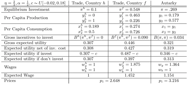
η=2₃, α= 1₂, c∼U[−0.02,0.18] Trade, Countryh Trade, Countryf Autarky Equilibrium Investment πh_{= 0.1 π}f _{= 0.548 π=.269}

Per Capita Production y

h

1 = 0

yh

2 = 1

yf

1 = 0.463

y₂f = 0.226

y1 = 0.179

y2 = 0.577

Per Capita Consumption x

h

1 = 0.189

xh

2 = 0.5

xf₁ = 0.274 xf

2 = 0.726

x1=y1

x2=y2

Gross incentives to invest Bh_(πh_{, π}f_{) = 0 B}f_(πh_{, π}f_{) = 0.090 B(π, π) = 0.034}

Gross expected utility 0.307 0.446 0.321 Expected utility net of inv. cost 0.308 0.427 0.319 Expected utility if invest 0.307−c 0.487−c 0.346−c Expected utility if don’t invest 0.307 0.397 0.313

Wages w

h g = 1

wh b = 1

wf

g = 1.875

wf_b = 1

wg= 1.364

wb= 1

Expected Wage 1 1.452 1.154 Prices p1= 2.648 p1= 3.216

Table 1: Trade and autarky equilibria in Example 1

Example 1: specialization may be beneficial only to the rich country

Table1displays a parameterization where all countryf citizens are better off in the asym-metric trade equilibrium than in the unique autarky equilibrium, and where all country h

citizens are worse off in the asymmetric trade equilibrium than under autarky.26

Notice that the total world output of both goods is higher in the asymmetric equilibrium (see the second row of the table). While prohibitive trade barriers would make country h

better off, it is also true that there exists transfer payments fromf tohthat can make both countries better off relative to the autarky equilibrium. Hence there are some productive gains from specialization despite the countries being fundamentally identical.

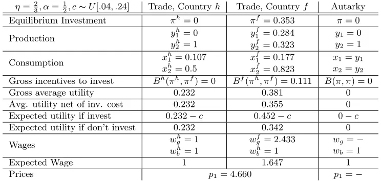
Example 2: specialization may make both countries better off

In this example trade makes both countries better off. For maximal simplicity we rig this example so that the “free rider problem” in human capital investments is so severe that the unique equilibrium under autarky is the trivial equilibrium. However, with trade, the existence of the other country means that, for any investmentπf _{in countryf, the price of} good 1 is higher than without trade if there is no human capital investment in country h. Hence, trade allows a new market to emerge that would not operate without trade.

In Table 2 we summarize one example where the market for good 1 only operates with

26_{Although some agents change their investment behavior in the comparison across equilibria, this does}

η= 2₃, α=1₂, c∼U[.04, .24] Trade, Countryh Trade, Countryf Autarky Equilibrium Investment πh_{= 0 π}f _{= 0.353 π= 0}

Production y

h

1 = 0

yh

2 = 1

yf

1 = 0.284

yf₂ = 0.323

y1= 0

y2= 1

Consumption x

h

1 = 0.107

xh

2 = 0.5

xf₁ = 0.177 xf

2 = 0.823

x1=y1

x2=y2

Gross incentives to invest Bh_(πh_{, π}f_{) = 0 B}f_(πh_{, π}f_{) = 0.111 B(π, π) = 0}

Gross average utility 0.232 0.381 0 Avg. utility net of inv. cost 0.232 0.355 0 Expected utility if invest 0.232−c 0.452−c 0−c Expected utility if don’t invest 0.232 0.342 0

Wages w

h g = 1

wh b = 1

wf

g = 2.433

wh b = 1

wg =−

wb= 1

Expected Wage 1 1.647 1

Prices p1= 4.660 p1=−

Table 2: Trade and autarky equilibria in Example 2

international trade. There are multiple trade equilibria and the numbers in the table refer to the equilibrium with the largest fraction of investors in the country producing good 1.27 Consumers are happier when consuming both goods than when consuming only one good. Because a new market opens up, trade is beneficial for both countries.

Pareto Improving Inequality

The example presented above is extreme, but specialization through trade may more gen-erally be viewed as an imperfect “solution” to the informational problem in the model.28

In the example, there is no way for a market to open unless the rewards for getting into the market are large enough. These rewards are bigger if only one country enters the market: the same “kick” from the local informational externality is generated at a smaller negative price effect. Specialization thus reduces the problem of under investment in human capital. Even in less extreme cases, both countries may gain from specializing: it isalways true that the production possibilities set expands when moving from a situation where both countries invest at the same rate to an asymmetric investment profile for a constant total quantity of investors in the world. Figure 9, assumes countries of equal size. In the left panel, the dashed line represents the frontier some symmetric investment profile with both countries investing atπ, whereas the continous lines (with kinks atB and C) illustrate the frontiers in each country at an asymmetric investment profile, but with the same aggregate investment.

On the right panel the continuous line (with kinks at D, AandE) represents the world

27_{There is also an equilibrium withπ}h_{= 0, π}f _{= 0.0157.Unlike the equilibrium in Table2this is unstable.}